an author's
https://oatao.univ-toulouse.fr/26908
https://doi.org/10.1016/j.ndteint.2020.102300
Bato, Miguel Reseco and Hor, Anis and Rautureau, Aurelien and Bes, Christian Experimental and numerical
methodology to obtain the probability of detection in eddy current NDT method. (2020) NDT & E International, 114.
102300-1023013. ISSN 0963-8695
Experimental and numerical methodology to obtain the probability of
detection in eddy current NDT method
Miguel Reseco Bato
a,b,*, Anis Hor
a, Aurelien Rautureau
b, Christian Bes
aaInstitut Cl�ement Ader (ICA), Universit�e de Toulouse, CNRS, ISAE-SUPAERO, UPS, INSA, Mines-Albi, 3 rue Caroline Aigle, 31400, Toulouse, France bAIRBUS OPERATIONS S.A.S., 316 route de Bayonne, 31060, Toulouse Cedex 09, France
Keywords:
Probability of detection (PoD) Human factors
Eddy current NDT simulation Device effect
A B S T R A C T
The scope of this paper is to define a methodology for building robust PoD curves from numerical modelling. First, an experimental database will be created in a laboratory scenario. A representative sample of inspectors with different certification levels in NDT method will be employed. Multiple inspections will be carried out to include the human influence in the MAPOD calculation. In addition, this study will take into account the impact of using different devices in the High Frequency Eddy Current method (HFEC). Then, a simulation model is created taking into consideration the main uncertainties due to human and device factors. These uncertainties are identified and quantified by the observation of experimental NDT inspection. Then, statistical distributions of these uncertainties are derived and used as inputs of the simulation model. Finally, the simulation PoD model will be compared and validated with the experimental results developed in the laboratory scenario. This com-parison provided encouraging results to replace or complete experimental tests by simulation.
1. Introduction
NDT reliability [1–5] is a key factor in ensuring the safety of struc-tural components. Currently in the aerospace field, this reliability is quantified through the Probability of Detection (PoD) which is the probability of detecting a defect as a function generally of its size [6]. The PoD curve can also be a function of the defect depth, skew or tilt but normally the defect length is the most representative measure [7]. Each NDT result is only valid for a geometry, a defect type, an inspection system and an associated procedure combination. However, one of the largest sources of variability during in-service inspections derives from human factors: an inspector performs the NDT calibration, the NDT scanning and interprets the signal response provided by the device including environmental and organizational factors [4,8,9]. Moreover, environmental conditions, protective clothing, time stress and organi-zational structure can affect the inspector’s performance, having an indirect impact on reliability [10]. Reliability can be impacted because having more NDT variables (environmental conditions, protective clothing, time stress and organizational structure) means a greater number of inspections have to be performed to observe and evaluate the influence of them all, in order to represent reality. Another variability
source hails from the device used in the NDT inspection and the signal response it generates. Therefore, the impact of each variability source is crucial in the process of better understanding NDT inspections.
The experimental determination of PoD curves is challenging due to the fact that a large number of tests must be performed in order to determine reliable results. A few studies [11,12] recommend the use of at least 60 target defects to obtain a robust PoD curve for the High Frequency Eddy Current (HFEC) method. In addition, each inspection has to be performed by a large number of inspectors under similar conditions, which incurs high costs and takes up significant time. However, the need for PoD data is becoming considerable since the use of probabilistic methods for safety justification is becoming widely accepted.
Today, due to pressure on cost and interval cycles, the aerospace industry is trying to replace the experimental data with simulated results for estimating PoD curves [13–15]. Several authors refer to the NDT simulation concerning PoD curves as MAPOD (“Model Assisted POD”) [16,17]. The full-model assisted POD, is a MAPOD approach which uses simulated NDT data as input for evaluation of the Probability of Detection [18–21]. Papers show examples of full-model assisted PoD on eddy currents or ultrasound inspection for artificial cracks using the * Corresponding author. Institut Cl�ement Ader (ICA), Universit�e de Toulouse, CNRS, ISAE-SUPAERO, UPS, INSA, Mines-Albi, 3 rue Caroline Aigle, 31400, Tou-louse, France.
E-mail address: [email protected] (M.R. Bato). https://doi.org/10.1016/j.ndteint.2020.102300
uncertainty propagation method. The majority of them compute simu-lation models integrating parameters in resimu-lation to the defect as the width, depth or skew; or in relation to the material as conductivity or structural noise [22–24]. Simulated PoD curves can avoid the major issue, which is the very high cost of experimental campaigns, which require production of a large set of representative defects and a large number of inspections of these defects. These PoD models are not compared and validated with the experimental database. The statistical laws for the uncertain parameters are chosen arbitrarily. There are few studies in the literature which analyze the impact of human factors and equipment on the reliability of the NDT process. In an experimental campaign, inspections not only depend on defect variability and mate-rial heterogeneity but also on the level of expertise of the inspector. This impact, which may affect the human operation part of the inspection, is indirectly linked to the inspector’s qualitative skills (experience, certi-fication level, mechanical knowledge, etc.). MAPOD studies [14,15] have so far generally refrained from incorporating human factors in MAPOD due to difficulties to model human behavior, which is always noted as a limitation.
In the approach presented hereinafter, the NDT simulation model has integrated human gestures (XYZ axis trajectories during the scanning path of the inspection) by modelling inspectors’ movements (probe angular positions and scanning increments) and not the human traits (experience, certification level, mechanical expertise, etc.). In addition, human gestures are impacted by the environment, inspection time (fa-tigue) and other factors.
In this paper the concept of “Model Assisted POD” is proposed in the case of High Frequency Eddy Currents (HFEC) method on artificial fa-tigue cracks. The probabilistic simulation model is used to take into consideration uncertainties due to human and device factors. These uncertainties are introduced as statistical distributions defined by NDT engineer experts and by observation of experimental NDT inspections. During this observation, the extended experimental database is devel-oped for two scenarios: same device and device switch. Then, this database is used to compare and validate the MAPOD.
The objectives of this paper are first, to establish a robust construc-tion of an experimental PoD curve applying the Berens Signal Response method; second, analyze the impact of different devices and third, define a methodology to design a numerical model based and validated using the experimental campaign. This numerical model integrates the human factors as human gestures (XYZ axis trajectories during the scanning path of the inspection) which represent the inspectors’ movements. This work aims to develop a simulation model to replace or complete the experimental PoD study. Thereby, PoD modelling can be used to reduce costs for the NDT reliability assessment.
This paper is organized as follows; the first section presents the basic concepts of Probability of Detection and details the Berens Signal Response Method. In section two we first describe the NDT procedure associated with eddy current. In the third section we present the eddy current simulation model built by CIVA software which uses the elec-tronic penetration theory coupled with boundary element methods. To deal with the uncertainties in relation to inspector skills, devices and specimen crack length based on engineering judgments, we introduce random variables on simulation inputs. Section four gives the experi-mental and simulation PoD results. Then, to see if the simulation can be replaced or completed with the experimental tests, we compare the PoD curves. Finally, the 6th section draws conclusions and addresses further research works.
2. Probability of Detection (PoD)
The Probability of Detection is used to determine the reliability and the capacity of the inspection device to detect defects according to their size for this aeronautical application case. PoD analysis is included in but not limited to verifying the reliability of an NDT inspection process. In general, such verification is required within the scope of a
qualification project. One of the most important PoD results is the defect size, whose Probability of Detection is 90% at a confidence level of 95%. Such a defect size is designated as “a90|95”. In general, the experimental
verification is considered as passed if the resulting “a90|95” is not greater than the relevant size.
The basis of the PoD procedure is the selection of the method to build the PoD analysis [26]. There are several possible methods to perform a PoD analysis [27]: 29/29 Method [28], Berens Hit/Miss Method, Berens Signal Response Method, Berens Signal Response Method with non-central t-distribution [2,29] and other methods. The 29/29 Method and the Berens Hit/Miss method are used for binary control data (defect detected → one, or defect not detected → zero). These methods are mainly used in visual inspection, penetrant tests, magnetic particle tests or X-Ray tests. The Berens Signal Response Method is used for amplitude control data. These results contain more information than one or zero (detect the defect or not) and they are mainly used in eddy currents and ultrasound testing. This method takes into account the signal response ba (i.e. the signal amplitude) of the detection caused by the defect of size “a”. In High Frequency Eddy Current method (HFEC), the type of resulting data include amplitude signals, therefore Berens Signal Response Method was selected for PoD curve building. In addition, this method remains correlated and consistent with the inspector amplitude results. This method was recommended by several studies [30–32]. The PoD curve was computed through parametric regression using maximum likelihood method, as a function of the data type.
The first steps in experimental or simulation PoD curve, consist of obtaining the experimental or simulated results which will feed the statistical method. In the experimental case, Fig. 1a shows how to construct the defect detections database from experimental samples. These results are obtained taking into account the variability due to inspector skills, devices and specimen crack. In the simulation case (Fig. 1,b1), uncertainties are introduced to compute the simulation database depending on the NDT engineering judgement and the obser-vations of experimental NDT inspections.
Then, the calibration step is performed to obtain the equivalence between simulated and detected amplitudes (Fig. 1,b2). Then, in both cases, the best linearity transformation is applied before using Berens Signal Response Theory to compute the PoD curve and the minimum detectable length (a90=95).
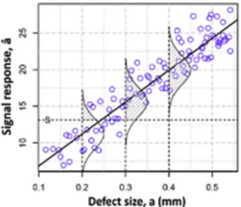
1. Data linearity: linear correlation between the defect detection (ba) and the defect size (a). In order to accept the PoD results, this cor-relation must follow the straight line defined by yi¼β0þβ1xiþεi
(see Fig. 2).
2. Homoscedasticity: Signal deviation gaps have to be the same for all sizes according to their average defect signal size. The scatter must be uniform all along the straight line defined by ba vs a. (see Fig. 2). 3. Residuals normality: residuals have to converge to their average
signal according to Gaussian distribution. The errors must be (approximately) normal. This condition is always met due to the Central Limit Theorem. Exceptions may occur when logarithmic transformation is needed to adjust the ba vs a relationship to yi¼β0þ β1xiþεi (see Fig. 2).
4. The observations must be uncorrelated. There should not be any influence on ba except the size, caused by, for example, changing device settings (e.g. EC probes).
After implementing the right transformation, the statistical process has to be continued with the Berens linearity equation (ba ¼ β0þβ1*a þ
δ). Actually, it is considered that a defect is detected when signal ba exceeds the decision value bath, which enables the Probability of
Detec-tion (PoD) to be defined as:
PODðaÞ ¼ pðba > bathÞ (1)
experimental data. These estimations can be obtained by maximizing the likelihood function L of n independent experiments [2]. Therefore, a PoD computation with unacceptable confidence level (e.g.: 95%) has to be generated. This defines,
PODðaÞ95%¼PODða hÞ ¼ Φ � loga bμ b r h � (2) Where, h ¼ � γ nk0 � 1 þðk0*bz þ k1Þ 2 ðk0*k2 k1Þ2 ��0:5 and bz ¼ loga bμ b σ (3)
γ is the solution of the following non-linear equation 1 2 � P x2 2�γ � þ2* Φ� ffiffiffip �γ 1 � (4)
k0, k1 and k2 are deduced from the I ¼ ðbβ0; bβ1; bσδÞobserved matrix.
In other words, there is only a 5% chance that the calculated a90=95 is
non-conservative compared to the unknown true value defect size a90. In
this study, the PoD curve module developed by Airbus will be used for the statistical analysis during evaluation of the Probability of Detection (PoD) in different scenarios.
3. Experimental tests
3.1. Eddy current NDT procedure
A development of an adequate procedure describing the instructions for determining an experimental PoD curve was established for the NDT procedures. This procedure was developed in such a way that it had to be representative of an in-service procedure focused on every instrument and material. In this paper, we discuss the High Frequency Eddy Cur-rents method. This procedure provides the standard requirements to inspect surface breaking cracks in different non-ferrous metals/alloys and glare materials.
In this study, the experimental NDT procedure is applied for poten-tial damage detection (fatigue surface cracks) in a flat plate made of titanium beta. This inspection is performed using an absolute mono-coil probe as the procedure specifies. This probe is connected directly to the device with an accuracy depending directly on each human as a result of being an in-service inspection. The eddy current control system com-prises the following:
- An eddy current generator capable of operating with an absolute probe at a frequency of 2 MHz, linked to the inspection (HFEC Method). Additionally, all inspection devices have to be internally verified (calibrated) in order to ensure proper use.
- An absolute probe of a fixed diameter (Ø 2 mm) with a general shape for suitable detection using the procedure.
- A calibration block, used for accurate measurement of surface cracks. The calibration block has certain dimensions and material specifi-cations similar to the inspection area in maintenance. From basic standards, the calibration block contains three different types of defects. Each defect consists of an “open” sleeve with three different
Fig. 1. Determination of the Probability of Detection (PoD) curves from (a) experimental database and (b) simulation database applying Berens Signal Response
method. To correctly apply Berens Signal Response Method [2], the statistical database must respect the following assumptions.
Fig. 2. Inspection Data for a statistical analysis following the Berens
depths respectively, machined by EDM (Electrical Discharge Machining) from titanium beta. The sleeve constitutes an infinite defect. The calibration block was used to define the structure noise threshold (banoise) and the saturation signal (basat).
Concerning the amplitude signals as inspection results, the defect characteristics can be correlated with the peak value of the signal from the high frequency eddy currents. Consequently, three areas in the de-vice screen, as a function of the amplitude signal, can be distinguished:
- First area, small defects in which no significant signal amplitudes are shown ðba < bathÞ, where, bath is the threshold signal used to obtain valid data. Usually this threshold signal corresponds to the structure noise threshold (banoise) or to a close value.
- Second area, bath< ba < basat, where basat is the saturation signal and is
directly related to the calibration procedure. In this second area, a relationship between the response signal ba and the crack size a is expressed.
- Third area in which the signal saturates. It normally concerns the larger and deeper defects ðbasat< baÞ.
Subsequently following the procedure, one essential and last point is the analysis of the tool to build PoD curves. This instrument shall be monitored in accordance with the applicable regulations (e.g.: Software verification, hardware check and best correlation).
The calibration step is important in order to properly assess the NDT results in each scenario. For this step, the inspector has to adjust the instrument parameters of the system to obtain a 100% FSH (Full Screen Height) for the NDT device, for the infinite defect at 1 mm depth on the calibration block. Then, this value is used to set up the 100% value in the PoD process which corresponds to the saturation threshold (basat). The
other important parameter is the detection threshold (bath) at 10% FSH as
the NDT HFEC procedure indicates. Actually, this bath is fixed once a
signal-to-noise ratio study has been carried out. This signal-to-noise ratio study allows inspectors to make the distinction between struc-ture noise and defects (acceptance criterion). Finally, the inspector passes the probe slowly along the area to inspect and checks that the coil scans the whole surface. All vertical indications exceeding bath (in this
case, 10% FSH) shall be marked as cracks. 3.2. Database construction
In this section, an extensive experimental database was set up. The objective is to provide a sufficient number of observations to identify PoD curves. Particularly in this study, 490 amplitude responses (ba) were used. These responses result from the control performed by seven in-spectors inspecting 70 samples. In the following lines, we describe the inspection scenarios performed, the samples used and the inspectors’ performances.
3.2.1. Inspection conditions
Several types and brands of detectors are used during detection op-erations. These different versions of devices can affect the variability of the detection results. To analyze these effects, two scenarios were considered while using the same samples. In addition, the same exper-imental conditions were applied to the inspectors. In the first scenario, the same equipment was used by the seven inspectors. However, in the second scenario, five different devices were used by the seven in-spectors: one per inspector. Then, two inspectors used two devices, whereas the remaining 5 inspectors each worked with one device. The two scenarios are illustrated in the following paragraphs.
- Same device scenario: This scenario is developed inside the non- destructive laboratory, where all specific inspections are performed according to facilities’ and device availability. This way of
performing a PoD curve study is common in the aerospace sector, as it is the easiest and quickest process. Inspectors begin their in-spections sitting down in a chair, with a high degree of comfort, without surrounding noise (laboratory environment) and standard temperature. Each inspector has to follow the NDT procedure, called HFEC NDT Instruction for TA6V Beta. This document provides the standard requirements for sample inspections in titanium beta alloy for the PoD process. Additionally, all inspectors in this case used the same device, Mentor EM Portable (noted D6), to only observe the human factors effect inside the laboratory scenario.
- Device switch Scenario: The experimental campaign is also devel-oped inside the non-destructive laboratory, where all specific in-spections are performed, as for the first test campaign. Each inspector has to follow the NDT general procedure as in the previous case. The difference is that in this analysis case, inspectors were using a different device to show the impact of this fact. For this reason, 5 HFEC devices are used in this scenario (D1 to D5). These devices are noted in the following order from D1 to D5; D1 - AeroCheck – Sofranel; D2 - Nortec 600 – Olympus; D3 – Elotest M2-Rohman GmbH; D4 – Elotest M3 - Rohmann GmbH and D5 – Phasec 2d. 3.2.2. Samples
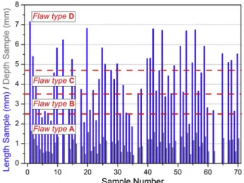
For this study case, the experimental test was run with 70 samples enclosing (or not) surface fatigue cracks, non-crossing thickness of a length (ls) of between 1 mm and 7 mm and variable depth. Defects should be as realistic as possible (fatigue defects) and moreover size distribution has been considered depending on the NDT method and the PoD scope. The rule is to provide the majority of defects having a size which is contained between a lower limit (defect size which can be detected with a low occurrence) and an upper limit (defect size which is in theory considered as always detected). Notice that samples with de-fects which are never detected and dede-fects which are always detected are also needed for the PoD study using Berens Signal Response Method. These fatigue cracks are accurately characterized using microscopy to be sure of inspectors’ detections and measurements (binocular inspection).
Fig. 3 provides the lengths (ls) and the depths (ds) measured.
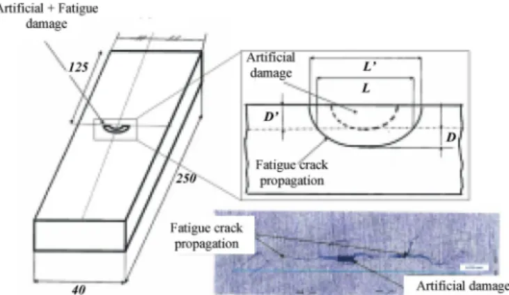
All inspection samples part of this PoD study are flat plates made of titanium beta. The fatigue propagation crack is initiated with artificial damage called EDM (Electro-Discharge Machining) followed by appli-cation of a three-point fatigue bending cycle. Once the fatigue defect in the surface plate has the desired length, the fatigue test is stopped and the sample is ready for trimming and engraving for the final inspection during the PoD study. The fatigue defect is the only defect existing for the PoD inspection, because the artificial defect was eliminated be-forehand in order to replicate actual in-service inspections (See Fig. 4).
Fig. 3. Sampling data clasified per defect type (length (ls) and depth (ds) vs.
After identifying the defect size as a function of its surface length, defects are characterized in 60 specimens (see Fig. 3). Within the experiment campaign, each sample has a different defect type to cover the PoD scope, except 10 of them, which are free of defects to prevent false calls. Probability of False Calls (PoFC) is a key parameter to take into consideration as part of reliability in PoD curves [2,12]. In addition, from the PoD hypothesis, at least 90% of the sample surface has to be free of defects for a correct study [12]. In total, the NDT inspection experiment comprises 70 samples manufactured in accordance with the design sketches.
3.2.3. Inspectors
For both scenarios (same device and device switch), twelve in-spectors in total carried out the HFEC inspections but only 7 per sce-nario. The number of inspectors carrying out the tests is an important parameter linked to reliability [33]. Then, the aim was to collect a sufficiently large and representative sample for these studies. For that purpose, we took 12 inspectors and we used the following parameters to explain how representative they are. Table 1 presents the inspector traits taken into account for the PoD curve analysis. These data are not used in the calculation for the PoD curve. The selected human characteristics are based on criteria analyzed in other studies [34] affecting NDT activity:
- Experience, being an important parameter for manual inspection. - Their mechanical expertise implies better understanding of each
NDT inspection process. Note that the marks assigned to each inspector were set up with a survey for this study.
Furthermore, some human characteristics were added based on several experimental studies developed by us where we assumed that the following may influence the inspections:
- Their certification level directly implies experience and knowledge on the fundamental parts of the NDT method.
- Right or left handedness which also has an influence in the probe angles due to the view position during the inspection.
The survey values illustrated in Table 1 were obtained from different qualification documents of each inspector and the questions answered by them. Their experience and certification level in eddy currents are based on inspectors’ answers, however, they were checked against the data stored in the NDT database. Mechanical expertise was evaluated with annual tests by means of several specific questions and evaluated according to a 10-point scale (highest mark). It was performed by Airbus to analyze their skills concerning damage propagation and fracture an-alyses. For example, in answer to the question as to their knowledge of the most influential parameters in the High Frequency Eddy Current method, inspectors will answer the defect parameters (length, depth or
width). To the same question, but in relation to damage propagation, the answer will be the material characteristics (grain, surface or treatment). This knowledge is important for the correct interpretation of the signal and defect propagation during NDT inspection. These data are only for illustrative purposes, to show that the inspector sample used is repre-sentative of a standard NDT maintenance company with all inspectors’ experience and level of qualification. Inspector performances and their corresponding marks are given in Table 1. Finally, two of them per-formed the test in both scenarios. Then, these inspectors (I4 and I5) used two devices (one device per scenario). This clarification is important to properly follow the experimental campaign run in both scenarios.
In-service inspections should take human and environmental factors into account to provide reliable PoD curves. The human factors most likely to affect a PoD ranges from simple misunderstanding of the pro-cedure by inspectors (including calibration and inspection methods) to the decision-making process, where the rejection/acceptance criteria are determined and the result recorded. In order to reduce these po-tential discrepancies, firstly, the procedure must be as clear and as un-ambiguous as possible and secondly, defects should not be of common knowledge between inspectors before inspecting each sample. Then, the set PoD has to simulate a real environment as closely as possible so that the inspector can perform the inspection as if they were carrying out his daily job inspecting parts [4,34]. In the following paragraph, the experimental results will analyzed in-depth.
3.2.4. Amplitude responses database
The amplitude database obtained directly from inspectors will be presented for each scenario. This analysis has to be performed before analyzing the PoD curves with the mathematical process and their sta-tistical parameters. The results from the two scenarios are illustrated in
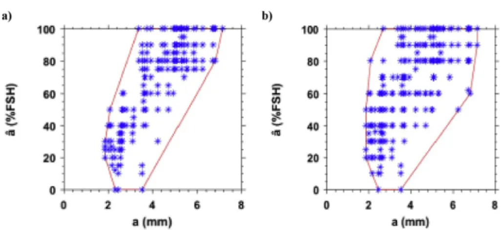
Fig. 5. The area in the device switch scenario is larger due to a higher variability and less repeatability in terms of amplitudes (Fig. 5b). It can be concluded that inspectors are less accurate in terms of detection due to the device switch effect. This impact is analyzed in this section in a general manner but more in-depth in the following sections and compared with the simulation model.
4. Eddy current NDT simulation modelling
CIVA NDE 2017 software is used to model the Eddy current NDT inspection [35]. This software is an expert digital platform for non-destructive testing. The software also provides a statistical analysis tool for construction of the Probability of Detection (PoD) curves based on the maximum likelihood method. The methodology used to obtain variability in inspection results, as in in-service inspections, is based on the introduction of uncertainty on different input parameters [36].
The High Frequency Eddy Current inspection model is presented in this section. In accordance with the experimental data base, the material is titanium beta (TAV6 Beta). The simulation geometry shape is a flat plate (250 � 40 � 5 mm). A semi-elliptical defect shape was used to resemble the experimental samples as closely as possible. In the actual samples the defect was characterized by a microscopy inspection and fracture analysis in ten titanium samples. The model chosen for the corresponding defect mesh will be the BEM (Boundary Element Method) because it is more representative of a real defect response (narrow de-fects). Finally, the simulated probe consists of one coil. The model is described in Fig. 6.
To corroborate the correspondence of the simulation model, to-mography was performed to analyze the HFEC probe. Nevertheless, an electromagnetic study was performed which confirms correct detection in titanium beta. Additionally, the electromagnetic penetration (mm) of eddy currents is studied [37]. The effective depth of penetration is the point in the material where eddy current strength has decreased to 37% of the strength at the surface. The effectiveness of the electromagnetic field computed by the CIVA model is close to 0.3 mm surface depth in titanium using a frequency of 2000 kHz. This value is similar to the
Fig. 4. Artificial and fatigue damage in a titanium beta specimen before
penetration depth obtained by the electromagnetic theory applied in pure titanium. Then, the simulation model can be considered to be similar to an in-service inspection.
4.1. CIVA model calibration
The objective of this section is to establish the equivalence between the experimental and numerical amplitudes. In the experimental sec-tion, the inspector has to adjust the system instrument parameters to obtain a 100% FSH and 10% FSH (Full Screen Height) as indicated in the HFEC procedure (described in Section 3). These parameters were called saturation threshold (basat) and detection threshold (bath) respectively.
This last parameter indicates the acceptance criteria.
The simulation calibration block has the same dimensions and ma-terial specifications as the experimental calibration block. In this
simulation model, the saturation value (basat) corresponds to a Y-axis
amplitude response of 1.43 mV (equivalent to 100% FSH in experiment) applying the correct phase and gain calibration. This process is similar to the inspectors’ experimental acquisitions for their calibrations. Then, taking 10% of this value (0,143 mV) we will define the detection threshold (bath).
4.2. Statistical description of CIVA uncertain parameters
In this section, we try to reproduce, through the simulation model, the PoD curve obtained from the experimental campaign, taking into account the uncertain parameters linked to the NDT inspection.
When performing an NDT inspection, the probe signal response varies due to an artificial or fatigue defect by mainly three factors, related to the inspection procedure specifications (transducer, cable, scan plan including transducer angles, electronic device), to the inspected part (geometry, material properties, surface treatment) and last but not least the defect (size, shape, orientation). Some of these parameters may be seen as uncertain if there is insufficient knowledge related to them, if they are not well-controlled during the inspection or if they imply physical phenomena with inherent randomness.
Firstly, all inspection parameters which are likely to represent sources of variability in the NDT results were identified by engineering judgment. Observation of the experimental campaign based on the NDT method of the application case enables good identification. A statistical description of each uncertain parameter identified must be prepared in order to feed the NDT computation model based on the MAPOD approach. Then, a sensitivity study was performed in relation to all HFEC parameters to quantify variability in terms of amplitude re-sponses. This sensitivity study was carried out using various influential parameters at the same time to observe correlations between them. This step is essential in terms of obtaining a reliable PoD curve and to know
Table 1
Inspectors’ performances in High Frequency Eddy Current inspection.
Inspector number Exp. Years in EC EC Level Mechanical Expertise (0-10) R/L handed Participant in Same device scenario Participant in Device switch scenario
I1 5 1 5 R yes no I2 26 2 9 R yes no I3 26 3 9 R yes no I4 10 2 7 R yes yes I5 27 2 7 R yes yes I6 20 3 7 L yes no I7 13 2 6 R yes no I8 4 2 5 R no yes I9 24 3 10 R no yes I10 17 2 10 R no yes I11 12 2 5 R no yes I12 25 2 8 R no yes
Fig. 5. Amplitude database areas from (a) same device scenario and (b) device switch scenario.
Fig. 6. Graphical representation of uncertain parameters in High Frequency
which parameters principally affect NDT detection.
For High Frequency Eddy Current (HFEC) method application cases, eight parameters have been identified as having a strong influence on the signal amplitude response. These eight parameters depend on the defect, the material and the inspector. These human parameters are identified and quantified in the recorded videos and the experimental campaign observation resulting from the inspectors’ movements. The movements counted during the HFEC inspections were the probe angles and displacements during the whole test, which are the raw data in degrees and millimeters. These human parameters are the human ges-tures of the NDT inspection (lift-off, the X and Y scanning increment and the X and Y angular position of the probe) integrated in the numerical model using the corresponding statistical laws.
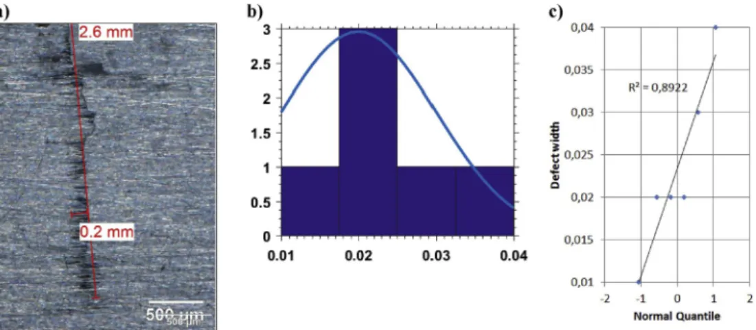
For example, the defect width (Table 2) is one of the parameters analyzed which was introduced as a statistical distribution in the nu-merical model. Then, using several experimental specimens observa-tions (Fig. 7a), the representative probability density function (PDF) was determined (Fig. 7b). The Henry’s law theory [38] was applied to demonstrate that the suppliers’ defect width measurements follow a truncated normal distribution in practice (Fig. 7c). The statistical pa-rameters of the truncated normal distribution are x ¼ 0:02 mm and
σ2 ¼0:01 mm. The defect width maximum and minimum correspond respectively to 0; 04 mm and 0:01 mm.
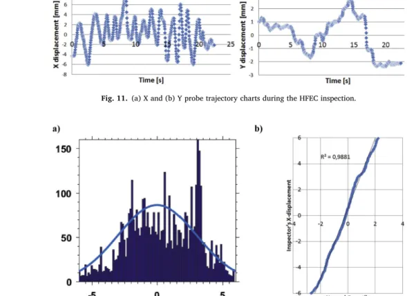
Another example is the inspector X rotation (rotation due to the inspector movement respect to the long sample axis, see Fig. 8). Several video acquisitions concerning the inspector X rotation are analysed for the Henry’s law theory which is presented below (see Fig. 9).
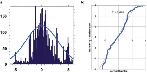
The last example is refers to numerous displacement acquisitions, which were obtained from the inspectors’ trajectory videos. For the numerical model, the X/Y displacements were indirectly introduced by changing the origin of the probe with a constant scanning path of 1 mm in each axis (X and Y), as the standard procedure describes. Actually, the simulation model gives a signal amplitude computation in each of these points for the proposed scanning path. Then, the uncertainty introduce through the probe origin (different probe origins) will generate different scanning paths and acquisition scanning points which is similar to how close the inspector was to the defect during the experimental inspection (Fig. 10).
In the following it can be observed the raw data used during the analysis to identify the statistical parameters for the inspectors’ trajec-tories (Fig. 11, Fig. 12 and Fig. 13).
These statistical laws were identified using the Henry law theory [38], which is a graphical method for fitting a series of observations by Gaussian distribution. The distributions used as inputs for the simulation study are described in Table 3.
The current numerical model assumes that the human traits (e.g. inspector’s experience, mechanical knowledge or procedure accuracy) during NDT inspections is globally represented by the human gestures. These human gestures modelled by the inspectors’ movements (X and Y rotations, X and Y displacements and lift-off) were determined experi-mentally during laboratory inspections using a representative popula-tion of inspectors.
5. Results and analysis
In this section, we will present the method we used to prepare the
data for the analysis, followed by the results and their interpretation. 5.1. NDT key parameters
For PoD curves, the parameters selected to analyze the realiability and effectiveness of the NDT method and the procedure are the following:
- a50 is the defect length for a 50% of Probability of Detection;
- a90 is the defect length for a 90% of Probability of Detection;
- a90=95 is the defect length for a 90% of Probability of Detection
ob-tained with a 95% confidence level.
These parameters are obtained from the inspectors’ detections in the two scenarios (same device and device switch) applying the Berens Signal Response method described in Section 2.
Once these statistical parameters are described for an in-depth analysis, for confidential reasons these PoD parameters are normalized by K. This normalization is also applied in the PoD curve axis. The normalized value of a50, a90 and a90=95 will be noted, respectively, a*50,
a*
90 and a*90=95. An example:
a*90¼a90
K (18)
Where K ¼ a90=95 ðsame deviceÞ, is the a90=95 obtained from the PoD curve
(linear-log scale) corresponding to the same device scenario. Addition-ally, the same normalization is applied in the PoD curve axis. This value is the baseline which is taken into account in aircraft interval in-spections. Then, PoD parameters can be presented and discussed following the example in each scenario.
5.2. Experimental PoD curves
In this section, PoD curve development is described step by step. The PoD programmer manager has to carefully follow this process to build an accurate PoD curve. This process is valid for each scenario previously described. In addition, this process will help us to address human ges-tures, environmental and device influence.
First of all, the NDT general procedure (HFEC inspection) describes the component or area to inspect such as fatigue test samples. Secondly, this document provides a description of potential damage in the form of fatigue cracks starting in the top surface of the fatigue test sample. Thirdly, the device and materials needed for inspection are described in detail (e.g. instrument, probe, calibration standard, supports, etc.). Before starting the inspection, inspectors have to verify the calibration date and conformity of the device; identify the area on the fatigue test sample to be inspected and check if it is clean and smooth. Another inspection is carried out in order to check for the absence of visible damage or discontinuities in each sample. In addition, an instrument calibration step has to be performed using the probe and the reference standard related to the inspection requirements in the general procedure.
5.2.1. Linearity study
In the following section we look at the linearity hypothesis of ba vs: a. Several transformations are used to obtain the correct linearity and maintain consistency with the Berens Signal Response hypothesis. In the literature, logarithm transformation is the most commonly used (i.e. log ðbaÞ vs a, ba vs log ðaÞ or log ðbaÞ vs log ðaÞ). Additionally, different al-ternatives can be proposed as transformations: square, square roots, exponential, etc.
The coefficient of determination is presented with the most relevant transformations to analyze the best option which fits with Berens line-arity hypothesis in same device scenario [39]. In addition, the same verification was performed in the case of the device switch scenario.
Table 2
Defect width corresponding to the experimental specimens. Defect Defect
1 Defect 2 Defect 3 Defect 4 Defect 5 Defect 6 Length
[mm] 1.85 2.2 2.62 4.3 5.84 6.95
Width
Finally, the coefficient of determination presented in Table 4 shows the best transformation which corresponds to linear-log for both scenarios. 5.2.2. Data homoscedasticity
Data homoscedasticity will also be treated as if it is one of the Berens hypothesis to be followed when building a reliable PoD curve. Homo-scedasticity consists of reaching the signal average for each defect size with an equal deviation. In actual fact, their deviation gap has to be uniform for all sizes in relation to their average size defect signal. With b
a vs: log a transformation, the main parts of amplitude detections are
inside the zone between the upper and lower deviation boundaries (red dotted lines in Fig. 14).
5.2.3. Residual normality
There are several methods for performing data normality. In this paper the Box-Cox transformation [40] was used to solve the residual normality problems. This transformation consists of transforming the Y variable, the sample values of which are assumed to be positive, otherwise a fixed quantity M is added so that Y þ M > 0. The Box-Cox transformation depends on a λ parameter to be determined and which
Fig. 7. (a) The width measurment (red line) of the specimen defect, (b) the defect width probability density function and (c) width distribution Henry’s line. (For
interpretation of the references to colour in this figure legend, the reader is referred to the Web version of this article.)
Fig. 8. (a) Frontal video view of the HFEC inspection and (b) the inspector’s X rotation analysis.
is given by Refs. [41]: Z ðλÞ ¼ 8 < : yλ 1 λ if λ 6¼ 0 logðyÞif λ ¼ 0 9 = ; (19)
If the objective is to transform the data to achieve normality, the best method to estimate the λ parameter is that of maximum likelihood. It is calculated as follows for different values of λ,
U ðλÞ ¼ 8 > < > : yλ 1 λ~yðλ 1Þ if λ 6¼ 0 ~ yðλ 1Þ logðyÞif λ ¼ 0 9 > = > ; (20)
where ~y ¼ ðy1y2…ynÞ1=n is the geometric mean of the variable Y. For each λ, we obtain the set of values fUðλÞgn
i¼1 . The likelihood function is:
LðλÞ ¼ n 2ln Xn i¼1 ðUiðλÞ UðλÞÞ2 ! (21) The bλ parameter is chosen to maximize LðλÞ. In practice, we compute LðλÞ in a grid of values of λ that allows us to approximately produce function LðλÞ and obtain its maximum.
~
λMV¼λ0 ; Lðλ0Þ �LðλÞ; 8λ (22)
After presenting the results of the BOX-COX transformation with their respective λ values in both scenarios (same device and device switch), we are able to evaluate whether each transformation will pro-vide a correct answer in terms of residual normality (See Table 5). For both scenarios the λ value is close to one, therefore applying the BOX- COX method will modify neither the residual nor the data. Finally, transformation ba vs log a makes it possible to respect the three previous Berens hypotheses (linearity, homoscedasticity and residual normality). Finally, note that the BOX-COX transformation which uses the geo-metric mean estimation has advantages and disadvantages [42]. The positive point is the simplicity of the calculus of the maximum likeli-hood. However, this rescaling model is not equivalent to the untrans-formed model since the procedure involves more than a unit change. In addition, interpretation of the parameters is not clear after such rescaling. Nevertheless, this transformation was applied through the data obtaining the same outputs.
5.3. Device switch effect
The PoD curves in the same device and device switch scenarios are computed using the method described in Section 2 and resulting from 70 samples inspected by seven inspectors (Fig. 15). The same device PoD
Fig. 10. Two different scanning paths due to the change of the probe starting
point with the corresponding computation points in the simulation model.
Fig. 11. (a) X and (b) Y probe trajectory charts during the HFEC inspection.
results are: a*
50 ¼0:63, a*90¼0:95 and a*90=95¼1 (Fig. 15a). The device
switch scenario PoD results are: a*
50 ¼0:56, a*90¼1 and a*90=95¼1:06
(Fig. 15b). Analysis of the statistical results allows for differentiation between the scenarios performed in the laboratory with the same device
and device switch. The a*
90=95 difference between scenarios is 6% using a
different device compared to the optimum case (same device scenario). Moreover, this difference is lower in a*
50 and a*90. To conclude, the use of
a different device can impact crack detection but not in a substantial manner for the current NDT method (High Frequency Eddy Current). This difference can also be a consequence of the inspector’s calibration which is a key step in the NDT inspection.
Moreover for two inspectors (Inspector 4 and Inspector 5), the graphs (Fig. 16) plot the amplitudes obtained with two different devices (D4/ D6 for inspector 4 and D5/D6 for inspector 5), and show that there is less dispersion in the case of each inspector using the D6. We firstly conclude that this device could provide accurate amplitudes independently of the inspector (Fig. 16). However, this conclusion is based only on two ob-servations, therefore more studies are needed to confirm this assump-tion. As it was remarked before, the cause could be how familiar each of them are with the device. Calibration can be different even following the same procedure, as can device sensitivity in electronically-different devices.
To conclude, the statistical parameters acquired from the individual PoD curves (inspector 4 using D4 and D6; inspector 5 using D5 and D6) are better from the inspectors using D6 which is mainly related to better detection of the defects. These values suggest that even for the same inspector and scenario as assessed in Fig. 16 for I4 and I5, results can mainly be affected by device technology. As a lesson learned, the same
Fig. 13. (a) Y-displacement probability density function and (b) Y-displacement Henry’s line in the laboratory scenario. Table 3
Statistical data distributions for uncertain parameters introduced in the model for a high frequency eddy current inspection.
HFEC Parameters Statistical
distribution Statistical data parameters Inspection Lift-off (μm) Uniform [0 mm,0,5 mm]
Angular position of the probe – Y rotation (�)
Gaussian [0�, 10�] Angular position of the
probe – X rotation (�)
Gaussian [0�, 10�] Scanning increment –
Step X (mm) Truncated Gaussian [1 mm, 3 mm] Scanning increment –
Step Y (mm) Truncated Gaussian [1 mm,1 mm] Defect Depth (mm) Truncated
Gaussian [1 mm, 0.5 mm] Skew (�) Gaussian [90�, 10�]
Width (mm) Truncated
Gaussian [0.02 mm, 0.01 mm]
Table 4
Proposed transformations following the linearity hypothesis for both scenarios. Transformation Same Device Scenario - R2 Device Switch Scenario - R2
linear-linear 0.6753 0.5402
linear-log 0.7161 0.5814
log-linear 0.4289 0.2916
log-log 0.4716 0.3156
squareroot-linear 0.7014 0.5655
Fig. 14. Linear-log transformation of data distribution from NDT inspectors in (a) same device scenario and (b) device switch scenario. Table 5
values and their corresponding BOX-COX transformations for inspector amplitudes in (a) same device scenario and (b) device switch scenario.
Scenario λ ba Transformation
Same device 0.98 ba
participants should be used in both scenarios to perform a complete comparison and extract global conclusions and not only two. The main reason for this limitation was the large amount of time and budget spent on performing all these tests in different places.
5.4. Numerical PoD curves
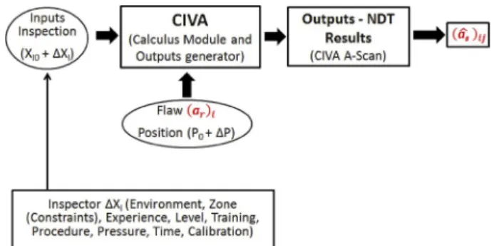
For numerical PoD curve development, a methodology will be fol-lowed to reproduce the impact of the variability of each parameter in-side the model. The variability represented on the NDT results from the simulation is statistically post-processed and used to calculate the nu-merical PoD curve. This reliable process follows the algorithm with a Monte Carlo sampling described in Fig. 17. Then, to construct this PoD curve, we need, for several values of ðaRÞi, to apply the procedure described in Fig. 17 and then obtain baij. Finally, after repeating this
procedure N times, the PoD curve is plotted (Section 2) using the defect lengths corresponding to the ðaRÞi ði¼1;…;NÞvalues and the defect ampli-tudes corresponding to baijði¼1;…;N; j¼1;…;MÞ.
The simulated detections vs. the artificial fatigue defect are illus-trated in Fig. 18. These results were obtained after introducing the variability sources and verifying the calibration step described in Sec-tion 2 and Fig. 1b. The simulation database gives a wider range of de-tections in comparison to the experimental database (illustrated in
Fig. 5a and b) thanks to the appropriate selection of statistical distri-butions related to uncertainties. Then, this conservative good agreement provides encouraging and promising results to replace or complete experimental tests.
Hence as previously, data linearity, homoscedasticity and residual normality are verified. The coefficient of determination R2 and λ
parameter are shown in Table 6.
After analyzing the hypotheses, the PoD curve is built to obtain the
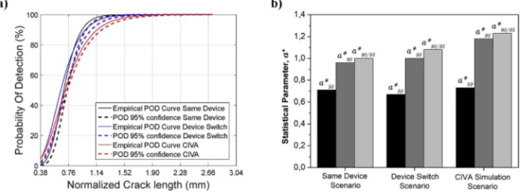
corresponding statistical parameters. Finally, the normalized PoD re-sults obtained from the simulation scenario are: a*
50¼0:73, a*90¼1:18
and a*
90=95 ¼ 1:23. The simulated PoD curve is compared to
experi-mental PoD curves in both scenarios (same device and device switch) in
Fig. 19a. Simulation and experimental statistical parameters can be assessed together (Fig. 19b). It should be noted that the simulation model produces conservative results compared to different scenarios (the minimum detectable length in the simulation is 23% greater than in same device scenario and 15% greater than in the device switch sce-nario). One of the main reasons may be that uncertain parameter de-scriptions were accurately selected in the CIVA model. These uncertainties are introduced as statistical distributions defined by expert NDT engineers and by observation of experimental NDT inspection (inspection videos) which are shown in Table 3, after thorough and careful analysis. This is a conservative approach as the inspectors’ values are usually better than the extreme values of the statistical distributions.
Fig. 15. PoD curve for a) same device and b) device switch scenario using titanium beta samples.
Fig. 16. Amplitude data for a) inspector 4 and b) inspector 5 obtained with different devices.
6. Conclusion
This study proposed a methodology for building robust PoD curves from numerical modelling. The application case deals with High Fre-quency Eddy Current based on the Berens methodology. The first step concerns experimental data which is used to validate our simulation model. Using the engineering judgment of NDT experts and observation of experimental NDT campaigns, we identified and quantified un-certainties due to different human gestures and device factors during the NDT process. These uncertainties are further characterized as statistical distributions. Then, using the Monte Carlo sampling method on these uncertainty distributions and running the deterministic numerical model we determined the different probabilities of detection lengths a*
50,
a*
90 and a*90=95. To compare experimental and numerical results, several
Berens hypotheses were analyzed from the signal amplitude data such as linearity, homoscedasticity and residual normality. The best trans-formation is ba vs: log ðaÞ for both experimental and simulation scenarios.
The difference between the experimental and simulation results on detection lengths a*
50, a*90 and a*90=95 never exceeded 23%. The minimum
detectable length computed by simulation PoD is greater than the experimental minimum detectable length. This parameter used for NDT
reliability in the in-service inspections defines the maintenance interval inspections. Using a greater value increases the number of inspections. Therefore, the simulation results are conservative in terms of detection thanks to the appropriate selection of statistical distributions related to uncertainties.
This conservative good agreement provides encouraging and prom-ising results to replace or complete experimental testing by simulations, which are less costly and time-consuming.
However, using Berens Signal Response method to build the PoD requires a good linearity relationship between the defect and detection. This hypothesis is debatable. In fact, the coefficient of determination (linearity indicator) is not close to the unit, especially in the case of simulation PoD studies. Thus, another statistical method should be considered [4].
In conclusion, the numerical model provides a conservative agree-ment although without taking human fatigue and stress due to 3–6 h of NDT laboratory inspection into account. This environment is not representative of real in-service inspections. In addition, the human gestures during NDT inspections are included with some limitations, such as the exact probe angle or position. Hence, further improvements can be proposed such as using powerful cameras to film the exact probe angle and displacements, or including a few gyroscopes on the probe for accurate measurements. Another model limitation is time in the random selection of each uncertain parameter computed by the Monte Carlo method. For the time being, the model is not able to run several com-putations at the same time. One improvement could be machine learning to perform smart random selection in parallel.
The NDT simulation model has integrated human gestures by modelling inspectors’ movements (probe angular positions and scanning increments) as the most practical method, extracted directly from the inspectors’ trajectories and gestures analyzed during the videos. This way of integrating human factors as gestures is new but we must be aware that is not a perfect match and that also it is not measured in this study. Human factors can have an effect on daily inspections. This is why the simulation results are not exactly the same as the experimental re-sults. One study limitation was not using the same inspectors for both scenarios (Same Device and Device Switch). The most appropriate method will be to use the same inspectors to learn more about the de-vices. In our approach we cannot conclude whether it is the people or the device that influence the results.
Future related work will attempt to extend our approach to broader- ranging NDT techniques (Ultrasonic, Radiography, Computed Tomog-raphy, Guide Waves, etc.) and in-service environments (aircraft main-tenance inspections). This research work will also include NDT problems where Berens assumptions are not fulfilled.
Declaration of competing interest
The authors declare that they have no known competing financial interests or personal relationships that could have appeared to influence
Fig. 18. Variability of the simulated detections corresponding to artificial
fa-tigue defects obtained using uncertain parameters.
Table 6
values and transformation for the BOX-COX method in the simulation scenario. Linearity transformation R2 λ values ba Transformation b
a vs log a 0:5208 0:92 ba vs: log a
the work reported in this paper.
CRediT authorship contribution statement
Miguel Reseco Bato: Methodology, Formal analysis, Investigation,
Writing - original draft. Anis Hor: Conceptualization, Methodology, Writing - review & editing. Aurelien Rautureau: Resources, Validation, Project administration. Christian Bes: Conceptualization, Writing - re-view & editing, Supervision.
Acknowledgements
This work would not have been possible without the “National Research Technology” association and Airbus Operations S.A.S.; which also enabled a research mission and several financial aids, devoted serenely to the development of my thesis.
References
[1] Department of Defense – United States of America. Aircraft structural integrity program (ASIP). MIL-STD-1530B 2004.
[2] Berens AP. NDE reliability data analysis. In ASM metals handbook: nondestructive evaluation and quality control. American Society of Metals International 1989;17: 689–701.
[3] Cheng RCH, Iles TC. Confidence Bounds for Cumulative distribution functions of continuous random variables. Technometrics 1983;25(1):77–86.
[4] Müller C, Bertovic M, Pavlovic M, Kanzler D, Ewert U, Pitk€anen J, Ronneteg U. Paradigm Shift in the holistic evaluation of the reliability of NDE systems. Materials Testing 2013;55(4):261–9. https://doi.org/10.3139/120.110433. [5] Holstein R, Bertovic M, Kanzler D, Müller C. NDT reliability in the organizational
Context of service inspection Companies. Materials Testing 2014;56(7–8):607–10.
https://doi.org/10.3139/120.110601.
[6] USA Department of Defense. Non destructive evaluation system reliability assessment. Department of Defense Handbook; 2009. MIL-HDBK-1823. [7] Pavlovi�c M, Takahashi K, Müller C. Probability of detection as a function of
multiple influencing parameters. Insight - Non-Destructive Testing and Condition Monitoring 2012;54(11):606–11.
[8] HSE. Reducing error and influencing behaviour. In: HSG48 (2. Edition). Health and safety Executive, HSE Books; 1999. Retrieved from, http://www.hse.gov.uk/pub ns/priced/hsg48.pdf.
[9] D’Agostino A, Morrow S, Franklin C, Hughes N. Review of human factors research in nondestructive Examination. In: Washington, DC: Office of Nuclear Reactor regulation, U.S. Nuclear regulatory Commission; 2017.
[10] Bertovic M, Gaal M, Müller C, Fahlbruch B. Investigating human factors in manual ultrasonic testing: testing the human factor model. Insight - Non-Destructive Testing and Condition Monitoring 2011;53(12):673–6.
[11] Cheng RCH, Iles TC. One-sided confidence Bounds for Cumulative distribution functions. Technometrics 2012;30(2):155–9.
[12] Gandossi L, Annis C. ENIQ report No 41: “probability of detection curves: statistical best-Practices”. EUR – Scientific and Technical Research series – ISSN 1018-5593, ISBN 978-92-79-16105-6 2010.
[13] Dominguez N, Reverdy F, Jenson F. POD evaluation using simulation: a phased array UT case on a complex geometry part. AIP Conference Proceedings 2014;1581 (1).
[14] Calmon P, Jenson F, Reboud C. Simulated probability of detection Maps in case of non-monotonic EC signal response. AIP Conference Proceedings 2015;1650(1): 1933–9.
[15] Li M, Meeker W, Thompson R. Physical model-assisted probability of detection of flaws in titanium forgings using ultrasonic non-destructive evaluation. Technometrics 2014;56:78–91.
[16] Online resources. Last accessed: May 2018, https://www.cnde.iastate. edu/MAPOD/.
[17] Li M, Meeker WQ, Thompson RB. Physical model-assisted probability of detection of flaws in titanium forgings using ultrasonic non-destructive evaluation. Technometrics 2014;56:78–91.
[18] Le Gratiet L, Iooss B, Blatman G, Browne T, Cordeiro S, Goursaud B. Model assisted probability of detection curves: new statistical tools and progressive methodology. J. Nondestruct. Eval. 2016;36:8. https://doi.org/10.1007/s10921-016-0387-z. [19] Subair SM, Rajagopal P. Simulation assisted determination of probability of
detection (PoD) curves: a short review. Indian Soc. NDT - J. NDE 2016;14(5): 66–73.
[20] Executive summary about the PICASSO project, web link. Last accessed: May 2018,
https://cordis.europa.eu/result/rcn/140492_es.html.
[21] Aldrin JC, Sabbagh HA, Murphy RK, Sabbagh EH, Knopp JS, Lindgren EA. Demonstration of model-assisted probability of detection evaluation methodology for eddy current nondestructive evaluation. In: Thompson DO, Chimenti DE, editors. Rev. Prog. Quant. Nondestruct. Eval. Burlington, VT: AIP Publishing; 2012. p. 1733–40.
[22] Calmon P, Jenson F, Reboud C. Simulated probability of detection Maps in case of non-monotonic EC signal response. AIP Conference Proceedings 2015;1650: 1933–9.
[23] Jarvis R, Cawley P, Nagy PB. Performance evaluation of a magnetic field measurement NDE technique using a model assisted Probability of Detection framework. NDT E Int 2017;91:61–70.
[24] Jenson F, Ammari H, Rouhan A, Dominguez N, Foucher F, Lebrun A, et al. The SISTAE project: simulation and Statistics for non destructive evaluation. 4th
European-American Workshop on reliability of NDE 2009. http://www.ndt.net/a rticle/reliability2009/Inhalt/th3a3.pdf.
[26] Guan X, Zhang J, Zhou S, Rasselkorde EM. Probabilistic modelling and sizing of embedded flaws in ultrasonic non-destructive inspections for fatigue damage prognostics and structural integrity assessment. NDT E Int 2014;61:1–9. [27] Rajesh SN, Udpa L, Udpa S, Nakagawa N. Probability of detection (POD) models for
eddy current NDE methods. Review of progress in Quantitative nondestructive evaluation. Adv Cryog Eng 1992;28:265–72.
[28] Friedman M. On the extended binomial distribution. Comput Oper Res 1984: 241–3.
[29] Kelley K, Cheng Y. Estimation of and confidence interval formation for reliability coefficients of homogeneous measurement instruments. Methodology 2011;8(2): 39–50.
[30] Yusa N, Chen W, Hashizume H. Demonstration of probability of detection taking consideration of both the length and the depth of a flaw explicitly. NDT E Int 2016; 81:1–8.
[31] Weekes B, Almond D, Cawley PBT. Eddy-current induced thermography- probability of detection study of small fatigue cracks in steel, titanium and nickel- based superalloy. NDT&E International 2012;49:47–56.
[32] Li M, Holland S, Meeker W. Quantitative multi-inspection-site comparison probability of detection for vibrothermography non destructive evaluation data. J Nondestr Eval 2011;30:172–8.
[33] Annis C, Gandossi L, Martin O. Optimal sample size for probability of detection curves. Nucl Eng Des 2013;232:98–105.
[34] McGrath B. Programme for the assessment of NDT in industry, PANI 3 [report No. RR617]. Health and safety Executive. Retrieved from, http://www.hse.gov.uk/ research/rrpdf/rr617.pdf; 2008.
[35] Calmon P, Chatillon S, Mahaut S, Raillon R. CIVA: an expertise platform for simulation and processing NDT data. Ultrasonics 2007;44(1):975–9.
[36] Jenson F, Iakovleva E, Dominguez N. Simulation supported POD: methodology and HFET validation case. AIP Conference Proceedings 2011;1335(1).
[37] Mook G, Hasse O, Uchanin V. Deep penetrating eddy currents and probes. Materials Testing 2007;49(5):258–64.
[38] Armatte M Robert. Gibrat et la loi de l’effet proportionnel. Math�ematiques et Science humaines – Ecole des hautes �etudes en science sociales 1995;129:5–35. [39] Hossjer O. On the coefficient of determination for mixed regression models. J Stat
Plann Inference 2008;138:3022–38.
[40] Chen G, Lockhart RA, Stephens MA. Box–Cox transformations in linear models: large sample theory and tests of normality. Can J Stat 2002;30(2):177–209. [41] Manorajan P, Sanjoy KP. Small sample estimation problem with BOX-COX
transformation: application to tea quality data. Statistica Applicata - Italian Journal of Applied Statistics 2000;12(3):377–92.
[42] Dagenais MG, Dufuor JM. Pitfalls of rescaling regression models with BOX-COX. Rev Econ Stat 1994;74(3):571–5.