Université de Montréal
Échantillonnage et modélisation de l’habitat des
communautés de poissons de rivière des basses
Laurentides
par
Jean-Martin Chamberland
Département de Sciences Biologiques, Université de Montréal Faculté des Arts et des Sciences
Mémoire présenté à la Faculté des Études Supérieures en vue de l’obtention du grade de
Maîtrise (M.Sc.) en Sciences Biologiques
Avril 2011
Université de Montréal
Faculté des études supérieures et postdoctorales
Ce mémoire intitulé :
Échantillonnage et modélisation de l’habitat des communautés de poissons de rivière des basses Laurentides
Présenté par : Jean-Martin Chamberland
Évalué par un jury composé des personnes suivantes :
Marc Amyot, président-rapporteur Daniel Boisclair, directeur de recherche
Résumé
Plusieurs études à grande échelle ont identifié la modification ou la perte d’habitats comme menace principale à la conservation des communautés de poissons d’eau douce. Au Canada, « aucune perte nette dans la capacité productive des habitats » (NNL) est le principe directeur de la politique de gestion des habitats du ministère des Pêches et Océans. Le respect du NNL implique l’avancement des connaissances au niveau des relations entre les poissons et leurs habitats, de même que des outils pour quantifier l’impact de la modification des habitats sur les poissons. Les modèles d’utilisation de l’habitat des poissons (FHUM) sont des outils qui permettent d’améliorer nos connaissances des relations poissons – habitat, de prédire la distribution des espèces, mais aussi leurs densités, biomasses ou abondances, sur la base des caractéristiques de l’environnement.
L’objectif général de mon mémoire est d’améliorer la performance des FHUM pour les rivières des basses Laurentides, en suggérant des perfectionnements au niveau de 2 aspects cruciaux de l’élaboration de tels modèles : la description précise de la communauté de poissons et l’utilisation de modèles statistiques efficaces.
Dans un premier chapitre, j’évalue la performance relative de la pêcheuse électrique et de l’échantillonnage en visuel (plongée de surface) pour estimer les abondances des combinaisons d’espèces et de classes de taille des poissons en rivière. J’évalue aussi l’effet des conditions environnementales sur les différences potentielles entre les communautés observées par ces 2 méthodes d’échantillonnage. Pour ce faire, 10 sections de rivière de 20 m de longueur ont été échantillonnées à l’aide de ces 2 méthodes alors qu’elles étaient fermées par des filets de blocage. 3 plongeurs performèrent l’échantillonnage en visuel en se déplaçant de l’aval vers l’amont des sections, tout en dénombrant les espèces et classes de taille. Par la suite, nous avons fait 3 passages de pêcheuse électriques et les abondances furent estimées grâce à un modèle restreint de maximum de vraisemblance, basé sur la diminution des abondances observées. De plus grandes abondances de poissons furent observées en visuel qu’avec la pêcheuse électrique à tous les sites. La richesse spécifique observée en visuel était plus élevée (6/10) ou égale (4/10) à celle observée avec la pêcheuse
électrique. Les différences entre les communautés de poissons observées à l’aide de ces 2 méthodes ne purent être reliées aux conditions environnementales. Les résultats de cette expérience sont contraires à ceux de toutes les études comparant ces 2 méthodes d’échantillonnage, lesquels suggèrent une supériorité de la pêcheuse électrique. Les conditions environnementales de notre expérience étaient distinctes de celles observées dans les autres études (absence d’arbres tombés dans l’eau, très peu de substrats grossiers), mais la différence la plus marquante était en terme de communauté de poissons observée (dominance des cyprinidés et des centrarchidés plutôt que des salmonidés). Je termine ce chapitre en suggérant que les caractéristiques comportementales favorisant l’évitement de la capture (formation de bancs) et facilitant l’observation en visuel (curiosité) sont responsables de la supériorité de la plongée de surface pour échantillonner les communautés dans les rivières des basses Laurentides.
Dans un deuxième chapitre, je développe des FHUM pour des communautés de poissons de rivière ayant plusieurs espèces. Dans le but de simplifier la modélisation de telles communautés et d’améliorer notre compréhension des relations poissons – habitat, j’utilise les concepts de guilde écologique et de filtre environnemental pour explorer les relations entre les guildes formées sur la bases de différents types de traits (reproducteurs, taxonomiques, éco-morphologiques et alimentaires) et les conditions environnementales locales à l’échelle du méso-habitat. Les modèles d’habitats basés sur les guildes reproductrices ont clairement surpassé les autres modèles, parce que l’habitat de fraie reflète l’habitat de préférence en dehors de la période de reproduction. J’ai également utilisé l’approche inverse, c’est à dire définir des guildes d’utilisation de l’habitat et les mettre en relation avec les traits des espèces. Les traits reliés à l’alimentation des poissons ont semblés être les meilleurs pour expliquer l’appartenance aux groupes d’utilisation de l’habitat, mais le modèle utilisé ne représentait pas bien la relation entre les groupes. La validation de notre modèle basé sur les guildes reproductrices avec un jeu de données indépendant pourrait confirmer notre découverte, laquelle représente une manière prometteuse de modéliser les relations poissons – environnement dans des communautés de poissons complexes.
En conclusion, mon mémoire suggère d’importantes améliorations aux FHUM pour les communautés de poissons des basses Laurentides, en suggérant de prendre en compte les caractéristiques biologiques des cours d’eau dans le choix d’une méthode d’échantillonnage, et également en utilisant une méthode prometteuse pour simplifier les FHUM de communautés de poissons complexes : les guildes reproductrices.
Mots-clés : Pêcheuse électrique, plongée de surface, centrarchidé, cyprinidé, rivière,
modèle d’habitat, méso-habitat, guilde reproductrice, alimentaires, éco-morphologique et taxonomique.
Abstract
Many large scale studies have identified habitat modification or habitat losses as primary threats for the conservation of freshwater fish communities. In Canada, No Net Loss (NNL) of the productive capacity of habitats is the guiding principle of the Department of Fisheries and Oceans’ policy for the management of fish habitat. To respect NNL, a better understanding of fish-habitat relationships is required, as well as tools to quantify the impact of habitat modifications on fish. Fish habitat use models (FHUM) are tools that can improve our understanding of fish-habitat relationships, predict species occurrences, densities or biomass on the basis of habitat descriptors and quantify habitat requirements. They consist in relationships between biological descriptors of fish and habitat descriptors.
The general objective of my thesis is to improve the performance of FHUM for the lower Laurentian streams by suggesting refinements on 2 crucial aspects in the development of these models: a precise description of the fish community and the use of efficient statistical models.
In the first chapter, I evaluate the relative performance of electrofishing and visual surveys (snorkeling) for estimating the abundance of combinations of fish species and size classes in rivers. I also assessed the effect of environmental conditions on potential differences between the results obtained using these two sampling methods. Sampling sites consisted in 10 river sections of 20 m in length distributed in the Laurentian region of Québec. Both methods were used while sections were blocked. Three snorkelers that swam the river sections upstream while identifying and counting fish of each species and size-classes performed visual surveys. Three-pass electrofishing was performed and abundances were estimated with a maximum likelihood depletion model. Greater abundances of fish were observed by snorkeling than by electrofishing at all sites. Snorkeling species richness was higher (6/10) or equal (4/10) to electrofishing richness. Differences in the fish communities observed by both sampling methods were not related to environmental conditions. The results of our work are therefore contrary to that of most published studies
that suggested the superiority of electrofishing on visual surveys. Compared to the conditions found in previous studies, our sampling sites had different environmental characteristics (no fallen trees, insignificant cover of large cobble and boulder) but the most striking dissimilarity was in terms of fish communities (dominance of cyprinids and centrarchids instead of salmonids). Behavioural characteristics favouring capture avoidance (schooling) and facilitating underwater observation (curiosity) may be responsible for the superiority of visual surveys in our study rivers. Survey methods should be selected based on fish community composition.
In the second chapter, I develop FHUM for complex stream fish communities. In order to simplify the modelling of such communities, as well as improve our understanding of fish – habitat relationships, I used the ecological guild concept and the niche filtering hypothesis to explore the relationships between guilds based on different types of traits (eco-morphological, reproductive, alimentary and taxonomic) and local environmental descriptors, at the coarse meso-habitat scale. Reproductive guilds led to FHUM that clearly outperformed the other 3 approaches, because of the close relationship between preferred spawning grounds and non spawning habitat preferences, and also because reproductive traits are linked to habitat characteristics at the reach or coarse mesohabitat scale. We also defined guilds based on habitat-use and related them to species traits. Traits related to the feeding biology of fishes seemed to be the best at explaining the habitat-use guilds, but our model did not correctly represent the among-guild relationships. Validation of our reproductive trait model on an independent dataset would confirm our finding, which represents a promising way of modelling fish - habitat relationships in complex fish communities.
In conclusion, my thesis suggests important improvements to FHUM models in the Laurentian streams by giving new insights on the choice of a sampling method that take into account the biological characteristics of the streams targeted, and by using a promising way of simplifying FHUM for species rich communities: reproductive guilds.
Keywords : Electrofishing, snorkeling, centrachid, cyprinid, stream, fish habitat use
models, guild, reproductive, alimentary, eco-morphological and taxonomic traits, meso-habitat
Table des matières
Page titre... i
Nomination du Jury ... ii
Résumé ... iii
Abstract ... vi
Table des matières ... ix
Liste des tableaux ... xi
Liste des figures ... xii
Liste des abréviations ... xiv
Remerciements ... xv
Avant propos ... xvi
Introduction générale ... 1
Chapitre 1: Comparison between electrofishing and snorkeling surveys conducted to describe fish assemblages in Laurentian Streams ... 7
Abstract ... 8 Introduction ... 9 Methods ... 11 Field surveys ... 11 Computations ... 15 Statistical analysis ... 15 Results ... 16 Discussion ... 22
Effect of abiotic conditions ... 23
Effect of biotic descriptors of fish communities ... 25
Chapitre 2: Comparison between different fish functional classifications to develop habitat use models ... 28
Abstract ... 29
Introduction ... 30
Study area ... 32
Sampling protocol ... 33
SPSC trait matrices ... 35
Computation and statistical analyses ... 37
- Relationship between guilds based on the diet, reproduction, eco-morphology and taxonomy, and habitat use ... 37
- Habitat use guilds and relationship with SPSC traits ... 41
Results ... 42
- Fish communities and local habitat descriptors ... 42
- Relationship between guilds based on the diet, reproduction, eco-morphology and taxonomy, and habitat use ... 45
- Habitat use guilds and relationships with species trait matrices ... 49
Discussion ... 54
- Comparison of the different guild to develop fish habitat models ... 54
- Habitat-use guilds and relationships with species traits ... 58
Conclusion ... 61
Conclusion générale ... 62
Références ... 70
Annexe 1 ... 82
Liste des tableaux
Chapitre 1
Table 1: Main abiotic and biotic characteristics of the sampling sites ... 13
Table 2: Species sampled, abbreviation and method with which the species was detected 17 Table 3: Cumulative adjusted r-square (R2adj), regression coefficients, standard error, t- and p-value of the forward selection of explanatory variables on MLR using snorkeling total fish abundance, snorkeling total fish abundance excluding fish of Size Class 1 and the Hellinger distance between the fish communities sampled by each method at each site as the response variables. ... 21
Table 4: Previous studies comparing snorkeling surveys with electrofishing ... 25
Chapitre 2
Table 1: Definition of the eco-morphological traits ... 35Table 2: Fish community characteristics... 44
Table 3: Main environmental conditions ... 45
Liste des figures
Chapitre 1
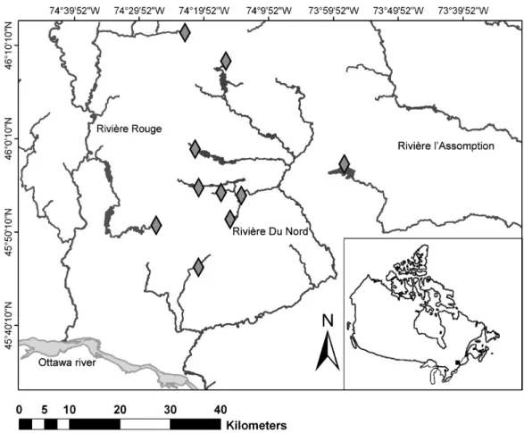
Figure 1: Map of the study area ... 12 Figure 2: Comparison of species richness observed by each sampling method at each site 18 Figure 3: Comparison of snorkeling total abundance and electrofishing estimated total abundance (a), and snorkeling abundance and electrofishing estimated total abundance excluding fish of size class 1 (b). ... 19 Figure 4: Frequency of the ratio of abundances (snorkeling / electrofishing) for each species ... 20 Figure 5: Principal component analysis on the covariance matrix of the 7 substrate classes (percent cover), scaling type 1. ... 20
Chapitre 2
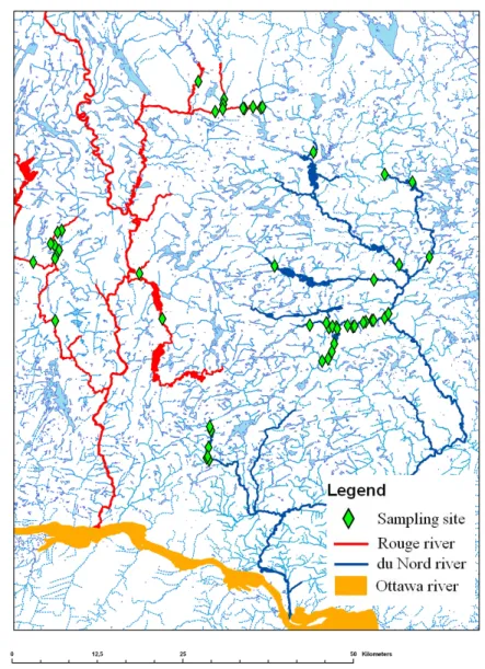
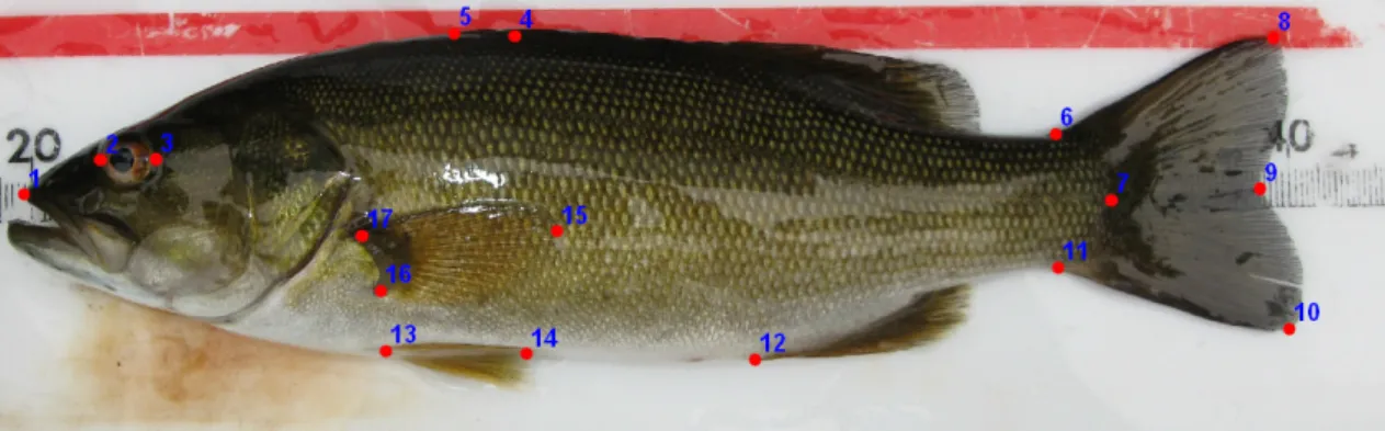
Figure 1: Distribution of the 50 sampling sites in the watersheds of Rivière Rouge and Rivière du Nord, Québec, Canada... 33 Figure 2: Position of the 17 landmarks used to calculate the 8 quantitative morphological traits. ... 37 Figure 3: Analytical framework ... 39 Figure 4: Principal component analysis performed on the covariance matrix of the percent cover of the 9 substrate classes. ... 46 Figure 5: R2adj of the relationship between the guilds formed based on alimentary, reproductive, eco-morphological or taxonomic similarities (A) and (B) average null models R2adj. ... 48
Figure 6: Triplot of the rda relating the 3 reproductive guilds to the forward selected local environmental descriptors. ... 49 Figure 7: Dendrogram of the habitat use guilds ... 50 Figure 8: Position of the habitat-use group centroids in the space of the 2 first linear discriminant axes ... 52 Figure 9: Multivariate classification tree 10 fold cross-validation relative error (±standard error; blue) (a) and multivariate classification tree selected following the Min + 1 SE rule (8 leaves) (b). ... 53
Liste des abréviations
≅ : approximately equal to CCR: Correct Classification Rate FHUM: Fish Habitat Use Models H0: Null Hypothesis
HM: Hydraulic Model
HSI: Habitat Suitability Index
LDA: Canonical Linear Discriminant Analysis MVCT: Multivariate Classification Tree NM: Null Model
NNL: Not Net Loss PC: Principal Component
PCA: Principal Component Analysis
PCNM: Principal Coordinates of Neighbour Matrices R2adj: adjusted R square
RDA: Canonical Redundancy Analysis RE: Relative Error
RLQ: R matrix Linked to Q matrix SD: Standard Deviation
SE: Standart Error
SPSC: Species and Size Classes TESS: Total Error Sum of Squares vs.: versus
Remerciements
Je tiens à remercier les personnes suivantes, car elles ont contribué tout au long de ma maîtrise à mon bonheur et à mon apprentissage. Tout d’abord, je tiens à remercier mon directeur de recherche, Daniel Boisclair, pour m’avoir permis de faire des études graduées, pour tout le temps qu’il m’a accordé, pour les connaissances et points de vue qu’il m’a partagés, ainsi que pour la grande confiance qu’il a eue en moi. Merci aux membres de mon comité, Marc Amyot et Nadia Aubin-Horth, pour avoir pris le temps de me faire des commentaires constructifs, lesquels ont permis d’améliorer significativement mon mémoire. Merci à Guillaume Bourque pour m’avoir enseigné une nouvelle langue, pour avoir grandement aidé à la collecte de mes données, pour avoir répondu à tellement de mes questions, pour son amitié, bref, pour avoir énormément contribué à mon projet de maîtrise. Je remercie aussi Gabriel Lanthier, Caroline Senay et Shannon O’Connor pour leur précieuse aide. Un gros merci à tous les « nouveaux » du labo parce qu’avec les « vieux », on est une belle gang! : Tom Bermingham, David Beauregard, Simonne Harvey-Lajoie et Camille MacNaughton. Merci à tous ceux qui m’ont aidé pour le travail de terrain : Florian Bonnaire, Jérémie Vernay, Stéphanie Massé, Olivier Houdoyer, Catherine Baltazar, Katerine Goyer, Irénée Sicard, Yohan Fittere, le personnel de la SBL et Louise Cloutier. Finalement, je tiens à dire un merci particulier à mes amis et à ma famille, que j’adore et qui m’ont soutenu tout au long de ma maîtrise, tout particulièrement Pierre-Yves Charpentier et Pierre-Luc Dézainde.
Avant propos
Ce mémoire a été rédigé sous forme d’articles dans le but éventuel de soumettre les 2 chapitres à des revues scientifiques internationales. L’auteur principal en est Jean-Martin Chamberland, lequel a élaboré en grande partie le projet, fait les revues de littératures, le travail de terrain (à l’exception des données décrivant les communautés de poissons et les conditions environnementales pour les 50 sites du chapitre 2), fait les plans d’analyse, la programmation des tests statistiques, la rédaction et la mise en page. Daniel Boisclair a encadré le projet tout au long de son avancement. Une version allongée des études est présentée dans ce mémoire, et les manuscrits devront être retravaillés par les 2 auteurs avant d’être soumis à une revue scientifique.
Introduction
Les écosystèmes aquatiques sont d’une importance capitale puisqu’ils fournissent de nombreux services, comme l’approvisionnement en nourriture, la régularisation de processus climatiques ainsi que plusieurs bénéfices non matériel tels les loisirs et le patrimoine culturel (Millenium Ecosystem Assessment 2005). Plus particulièrement, les poissons fournissent à l’ensemble de la population mondiale 16% des protéines d’origine animale (FAO 1997) et environ 1 milliard de personnes à travers le monde dépendent des poissons comme première source de protéine animale (FAO 2000). Les poissons d’eau douce constituent également une ressource renouvelable importante, puisqu’ils représentent plus de 26% des pêcheries mondiales (IUCN 2006), en plus de jouer des rôles écologiques essentiels au bon fonctionnement de ces écosystèmes, comme le stockage, le transport et le recyclage des éléments nutritifs (Vanni 2002).
En dépit de leurs importants rôles économiques, culturels et biologiques, plus de 20% des espèces de poissons d’eau douce ont subit un sérieux déclin ou se sont éteintes (Moyle et Leidy 1992). En Amérique du Nord, le nombre d’espèces de poissons d’eau douce considérées comme en danger de disparition, menacées, ou préoccupantes a augmenté de 251 à 364 dans les années 1980 (Williams et al. 1989). Plusieurs études (Miller et al. 1989; Williams et al. 1989; Noss et Cooperrider 1994; Allan et Flecker 1993; Naiman et al. 1995, Richter et al. 1997), bien qu’elles varient dans la finesse de la description des menaces à la conservation des poissons, s’accordent pour dire que les plus importantes menaces peuvent être catégorisées de la sorte : destruction et fragmentation des habitats, pollution et introduction d’espèces exotiques. Par exemple, dans une analyse portant sur l’extinction des espèces Nord Américaines de poissons, Miller et al. (1989) a conclu que l’altération physique des habitats était la cause la plus fréquente (contribuant dans 73% des cas) des extinctions d’espèces appartenant à la faune aquatique d’eau douce, suivi par l’introduction d’espèces envahissantes, l’altération chimique des habitats, l’hybridation et finalement la surpêche.
Plusieurs études à grande échelle ont donc identifié la modification ou la perte d’habitats aquatiques comme facteurs primaires menaçant la conservation des populations
et communautés de poissons d’eau douce (Williams et al. 1989; Allen et Flecker 1993; Richter et al. 1997). Au Canada, pour contrevenir à cette importante menace, le ministère des Pêches et Océans a pris le « No Net Loss of the productive capacity of habitats » (NNL; aucune perte nette en capacité productive des habitats) comme principe directeur de sa politique de gestion de l’habitat du poisson (DFO 1986). Le respect de cette politique implique d’être capable d’estimer la capacité productive en poisson d’un système non impacté, de prédire le changement en capacité productive causé par la perturbation, et finalement, que la différence entre la capacité productive avant et prédite soit de zéro. Conséquemment, le respect du NNL nécessite une excellente compréhension des relations entre les poissons et leurs habitats, de même que des outils pour quantifier les impacts des modifications de l’habitat sur la faune ichthyenne.
Les modèles de l’habitat des poissons (MHP) sont des relations mathématiques entre un descripteur biologique des poissons (e.g. biomasse, densité de poissons) et des descripteurs de l’habitat (e.g. la température de l’eau, la vitesse du courant, la profondeur de l’eau, etc.) (Barry 2006). Ce sont justement des outils qui permettent d’améliorer notre compréhension des relations entre les poissons et leurs habitats, ainsi que de quantifier les besoins en habitat (Ahmadi-Nedushan et al. 2006, Boisclair 2001). En milieu lotique, il est possible de prédire les effets des modifications de l’habitat sur les poissons en utilisant les prédictions d’un modèle hydrodynamique (e.g. la profondeur et la vitesse du courant) dans un MHP (Bovee et al. 1982, Nestler et al. 1989, Guay et Boisclair 2001) et ainsi obtenir une prédiction de la réponse des poissons aux modifications de leur environnement.
L’objectif général de mon mémoire est donc d’améliorer la performance des modèles de l’habitat des poissons, plus particulièrement pour les rivières des basses Laurentides. Dans chacun de mes 2 chapitres de mémoire, je montre comment améliorer un aspect d’importance particulière pour la création de ces modèles, soit la description adéquate de la communauté de poissons en place et les modèles statistiques utilisés.
Dans mon premier chapitre, je compare la performance relative de 2 méthodes d’échantillonnage communément utilisées pour décrire les communautés de poissons en
rivière : la pêcheuse électrique portative et la plongée en surface. Ces 2 méthodes présentent chacune leurs avantages et inconvénients. Par exemple, la pêcheuse électrique est moins affectée par la transparence de l’eau et la complexité de l’habitat que la plongée en surface (Gardiner 1984; Schill et Griffith 1984; Thurow et al. 2006), et elle permet aux opérateurs d’identifier précisément et de mesurer les poissons recueillis (Nordwall 1999). La plongée de surface, quant à elle, présente l’avantage d’être moins affectée par la profondeur, la vitesse du courant et la conductivité de l’eau que la pêcheuse électrique (Schill et Griffith 1984; Bonneau et al. 1995). De plus, la plongée de surface requiert beaucoup moins de temps et d’équipement que la pêcheuse électrique, ce qui la rend particulièrement appropriée pour l’échantillonnage de sites difficilement accessibles (Hankin et Reeves 1988; Thurow 1994). Cependant, lors de l’échantillonnage en plongée, il est possible de compter les poissons plus d’une fois, de même que de surestimer leur taille réelle (Griffith 1981).
Les études comparant ces 2 méthodes d’échantillonnage en rivière mènent habituellement à la conclusion que la pêcheuse électrique permet d’observer de plus grandes abondances de poissons que la plongée en surface (e.g. Cunjak et al. 1988, Hankin et Reeves 1988, Thurow et Schill 1996, Mullner et al. 1998, Wildman et Neumann 2003, Thurow et al. 2006, Roni et Fayram 2000), ce qui suggère que la pêcheuse électrique est une meilleure méthode d’échantillonnage que la plongée de surface.
Il est bien connu, cependant, que l’efficacité d’une méthode d’échantillonnage peut être reliée à la composition de la communauté de poisson, de même qu’aux conditions environnementales (Reynolds 1996). Par contre, toutes les études comparant la pêcheuse électrique portative et la plongée de surface en rivière que nous avons recensées ciblaient les communautés de poissons avec une faible richesse spécifique, dominées par les salmonidés, de même que les rivières caractérisées par une dominance de substrats grossiers et des températures froides.
Le premier objectif de mon premier chapitre est donc d’évaluer la performance relative de la pêcheuse électrique portative et de la plongée de surface pour estimer
l’abondance des espèces et classes de taille, et ce pour des communautés de poissons de rivière non dominées par les salmonidés. Le second objectif de ce même chapitre est d’évaluer l’effet des conditions environnementales sur les différences potentielles entre les communautés observées avec ces 2 méthodes.
Dans mon second chapitre, j’utilise le concept de guilde écologique (Austen et al. 1994), de même que celui des filtres écologiques agissants sur les traits fonctionnels des espèces (Smith et Powell 1971, Soutwood 1988, Zobel 1997), pour améliorer les modèles d’habitats des communautés de poissons de rivière des basses Laurentides.
La principale motivation pour appliquer ces concepts aux MHP est que le développement de tels modèles dans les communautés de poissons à forte richesse spécifique est très demandant, particulièrement en considérant que les besoins en habitat de plusieurs espèces de poissons changent tout au long de leur ontogénie (Hoagstrom et al. 2008; Weaver et al. 1997; Lamouroux et al. 2006). Une façon de simplifier l’élaboration de MHP dans de telles communautés est de grouper les espèces exploitant des ressources similaires en guildes, puisque ces espèces devraient être affectées de la même façon par des changement dans ces mêmes ressources (Roberts et O’Neil 1985).
Le concept de guilde fut originalement défini par Root (1967) comme un groupe d’espèces exploitant la même classe de ressources environnementales de façon similaire. Plus tard, Austen et al. (1994) proposèrent d’utiliser les guildes qui fonctionnent comme des « super espèces », une unité taxonomique se situant entre l’espèce et la communauté, et qui répondraient aux changements environnementaux d’une manière plus facilement prévisible que les membres individuels d’une espèce.
Le concept de filtre écologique, quant à lui, fut inspiré des idées de Southwood (1977, 1988), qui argumentait que les habitats agissent comme des cadres à l’intérieur desquels l’évolution forge les attributs phénotypiques des espèces présentes. Le concept de filtre écologique consiste donc à voir les caractéristiques des habitats comme des filtres qui imposent des contraintes aux espèces et sélectionnent ainsi les traits adaptés aux conditions environnementales présentes (Diaz et al. 1998). Ce concept suggère donc que les espèces
présentes dans les mêmes habitats seront plus semblables entre elles qu’anticipé par la chance.
Plusieurs approches existent pour former des guildes. En rivière par contre, l’utilisation des ressources par les poissons a été résumée sur la base de l’utilisation de l’habitat (Leonard et Orth 1988, Vadas et Orth 2000, Persinger et al. 2003), l’alimentation (Grossman et al. 1982, Angermeier et Karr 1983, Auster et Link 2009, Specziar et Rezsu. 2009) et les stratégies liées à la reproduction (préférence de substrat pour la fraie et comportement lors de la fraie ; Balon 1975). Une autre approche pour former des guildes consiste à grouper les espèces en se basant sur leurs traits éco-morphologiques, pour les raisons mentionnées plus haut, mais aussi parce que la morphologie reflète d’une certaine manière l’alimentation et l’utilisation de l’habitat (Bertrand et al. 2008; Reyjol et al. 2008; Bellwood et al. 2002; Wainwright 1996; Borcherding et Magnhagen 2008; Wikramanayake 1990; Chuang et al. 2006; Morinville et Rasmussen 2008).
À l’échelle du méso-habitat, la modélisation de l’habitat des poissons par guildes présente plusieurs avantages. Cette approche permet de faire des MHP plus constants, puisqu’ils sont calibrés sur des jeux de données comportant moins de zéros (Fausch et al. 1998). Lorsque utilisés conjointement avec les modèles hydrodynamiques pour déterminer les régimes hydriques nécessaires au maintien des populations, cette approche permet de protéger une plus grande proportion de l’écosystème impacté, puisqu’une plus grande proportion de la communauté de poisson est considérée (Vada et Orth 2001). Finalement, les prédictions des MHP basées sur une seule espèce sont moins précises parce que les abondances ou densités d’une espèce fluctuent beaucoup plus en fonction des changements biotiques et abiotiques que les abondances ou densités d’une guilde au complet (Orth 1995, Vadas et Orth 2000).
Le premier objectif de mon second chapitre est donc de comparer 4 différentes manières de former des guildes (par traits reproducteurs, alimentaires, éco-morphologiques et taxonomiques), et identifier la méthode qui permet de produire les meilleurs modèles d’habitat des poissons. Le second objectif est de définir a priori des guildes d’utilisation de
l’habitat et d’utiliser une forme de régression linéaire pour déterminer quels traits définissent le mieux ces guildes d’utilisation de l’habitat.
Comparison between electrofishing and snorkeling
surveys conducted to describe fish assemblages in
Laurentian Streams
Jean-Martin Chamberland and Daniel Boisclair
Université de Montréal, Département de sciences biologiques, C.P. 6128, Succursale Centre-ville, Montréal, Québec, Canada H3C 3J7
Contribution to the programme of GRIL (Groupe de Recherche Interuniversitaire en Limnologie et en environnement aquatique).
Abstract
We evaluated the relative performance of electrofishing and visual surveys (snorkeling) for estimating the abundance of combinations of fish species and size classes in rivers. We also assessed the effect of environmental conditions on potential differences between the results obtained using these two sampling methods. Sampling sites consisted of 10 river sections of 20 m in length distributed in the Laurentian region of Québec. Both methods were used while sections were blocked. Three snorkelers swam the river sections upstream while identifying and counting fish of each species and size-classes performed visual surveys. Three-pass electrofishing was performed and abundances were estimated with a maximum likelihood depletion model. Greater abundances of fish were observed by snorkeling than by electrofishing at all sites. Snorkeling species richness was higher (6/10) or equal (4/10) to electrofishing richness. Differences in the fish communities observed by both sampling methods were not related to environmental conditions. The results of our work are therefore contrary to that of most published studies that suggested the superiority of electrofishing on visual surveys. Compared to the conditions found in previous studies, our sampling sites had different environmental characteristics (no fallen trees, insignificant cover of large cobble and boulder) but the most striking dissimilarity was in terms of fish communities (dominance of cyprinids and centrarchids instead of salmonids). Behavioural characteristics favouring capture avoidance (schooling) and facilitating underwater observation (curiosity) may be responsible for the superiority of visual surveys in our study rivers. Survey methods should be selected based on fish community composition.
Introduction
Estimating the abundance of populations is crucial to assess their ecological status (endangered, threatened, etc; COSEWIC 2010), their potential role in food web (predator, prey, competitor; Polis and Winemiller 1996), and their capacity to sustain exploitation (fishing, hunting, harvesting; Pine et al. 2001; Krebs 2009). Electrofishing and snorkeling are two methods commonly used to estimate fish abundance in shallow areas (depth <2m) of rivers and lakes (Joyce and Hubert 2003; Mullner et al. 1998; Brind’Amour and Boisclair 2004). These methods have been used to study population dynamics (Sabaton et al. 2008; Petty et al. 2005) and to develop habitat use models (Bouchard and Boisclair 2008; Hrodey and Sutton 2008; Hedger et al. 2006).
Electrofishing has been argued to be less affected by water transparency and habitat complexity (e.g. substrate composition and macrophyte cover; (Gardiner 1984; Schill and Griffith 1984; Thurow et al. 2006) than snorkeling. Electrofishing also allows operators to precisely identify and measure the fish that are sampled and to estimate fish abundance using robust mathematical models (depletion estimates; Nordwall 1999). However, this sampling method may injure or kill fish and may have low capture efficiency, particularly for small fish (Reynolds 1996). In contrast, snorkeling has the advantages of being less affected by water depth, velocity, and conductivity than electrofishing (Schill and Griffith 1984; Bonneau et al. 1995). Nonetheless, during snorkeling, fish may be counted more than once and length estimates may be biased because of underwater magnification (Griffith 1981). Snorkeling surveys require modest equipment and less time than electrofishing, which makes it suitable to study remote locations (Hankin and Reeves 1988; Thurow 1994). Considering the importance of estimating fish abundance and the number of advantages and drawbacks associated with electrofishing and snorkeling, the identification of the most adequate survey method to estimate fish abundance in shallow waters is not a trivial problem.
Comparative studies typically lead to the conclusion that electrofishing permits the estimation of fish abundances that are higher than snorkeling. Cunjak et al. (1988) found that snorkeling underestimated the densities of juvenile Atlantic salmon (Salmo salar) and blacknose dace (Rhinichtys atratulus) compared to electrofishing. However, estimates of brook trout (Salvelinus fontinalis) population size were very similar between the two methods. Hankin and Reeves (1988) found that underwater surveys underestimated 1+ coho salmon (Oncorhynchus kisutch) and steelhead trout (Oncorhynchus mykiss) abundances relative to electrofishing in 13 sites out of 21, but that abundances obtained with both methods were generally well correlated (r > 0.90). Thurow and Schill (1996) concluded that snorkeling surveys were suitable for estimating the relative abundance and size structure of age 1+ bull trout (Salvelinus confluentus), but that snorkeling surveys underestimated abundances obtained using electrofishing by 25%. In their study on brook, rainbow (Oncorhynchus mykiss), and cutthroat (O. clarki) trouts, Mullner et al. (1998) found that trout abundances estimated with snorkeling were highly correlated (0. 90< r2 <0.99) to values obtained using electrofishing (depletion estimates) but that snorkeling counts underestimated electrofishing counts by 35%. Wildman and Neumann (2003) compared the abundance and the size structure of brook and brown trouts (Salmo trutta) obtained by snorkeling and electrofishing. They found that snorkeling averaged 66% of depletion estimates obtained using electrofishing, but that overall, length–frequency distributions obtained by snorkeling were similar to those obtained by electrofishing. Thurow et al. (2006) also found that snorkeling surveys tended to underestimate counts of three salmonid species (bull, cutthroat and rainbow trout) compared to electrofishing depletion estimates, with snorkeling going up to a maximum of 33% of electrofishing estimates. Roni and Fayram (2000) compared the relative efficiency of snorkeling and electrofishing depletion estimates for estimating the abundances of juvenile coho salmon and trouts (Oncorhynchus spp.). Night snorkel counts were not significantly different from electrofishing estimates, although the percentage of electrofishing estimates accounted for by night snorkeling varied among streams from 50% to 175% for coho salmon and from 75% to 82% for trout. At high fish densities (>0.5fish/m2), night snorkel counts
underestimated juvenile coho salmon abundance. However, at low densities (below 0.5 coho salmon/m2), night snorkel counts were often equal to or higher than electrofishing estimates. Most studies conducted to date to compare electrofishing and snorkeling surveys therefore indicate that electrofishing provides higher fish abundances than snorkeling and, hence, that electrofishing may be a more suitable method to estimate fish abundance than snorkeling.
It has long been recognized that the efficiency of a sampling method may be related to the composition of the fish community sampled (species, fish size, behaviour, etc) and the environmental conditions that prevail at sampling sites (water conductivity, temperature, presence of cover, etc; Reynolds 1996). Most comparative analyses of abundance estimates based on electrofishing and snorkeling have targeted fish communities with low species richness and dominated by salmonids and rivers characterised by coarse substrate and cold water temperatures. Hence, it is presently difficult to select the most appropriate sampling method to estimate fish abundance for other types of fish communities and environmental conditions. Therefore, the objectives of this study were to (1) evaluate the relative performance of electrofishing and snorkeling for estimating the abundance of fish species and size classes for non-salmonid communities and (2) to assess the effect of environmental conditions on potential differences between the results obtained using these two methods.
Methods
Field surveyElectrofishing and snorkeling surveys were done in 10 river sections distributed in the watersheds of Rivière Rouge, Nord, and l’Assomption (Figure 1). These rivers flow in the Lower Laurentian region of Québec and eventually drain into the Saint-Lawrence River. River sections were chosen to represent the range of fish community structures and habitat characteristics found in the region (Table 1). Surveys were conducted from the 2nd to the 14th of August 2009, between 10h00 and 16h00 to avoid diel differences in fish
habitat use and also because, in species rich communities, fish identification is easier in good light conditions. Sampling was conducted on days without rain and with a cloud cover not exceeding 50%.
Table 1 Main abiotic and biotic characteristics of the sampling sites Descriptors Mean Range
Stream width (m) 7.9 4.2 - 12.3 Mean depth (m) 0.54 0.43 - 0.64 Flow velocity (cm/s) 24.8 14.2 - 54.0 Dominant substrates (%) Clay - Silt (< 2 mm) 28 1 - 90 Sand (< 2 mm) 37 5 - 88 Gravel (2-32 mm) 15 0 - 40 Macrophyte cover (%) 20 0 - 56
Trunks (number of) 6 0 - 15
Water temperature (°C) 19.9 17.3 - 21.0
Conductivity ( µsiemens) 58 31- 92
Individuals belonging to (%)
Cyprinids 75 38 - 100
Centrarchids 18 0 - 52
Surveys were performed by blocking fish passage upstream and downstream a 20 m long river section using two 20 m long by 2 m high (mesh size = 2 cm) seines set perpendicularly to river shore (from shore to shore). Seines were held in place using wooden poles stuck in the riverbed after the setting of the nets. River sections of 20 m were used because this length corresponded to the longest section that could be surveyed without excessive clogging of the seines during the surveys.
Once the block nets were set, a 30 to 45 minutes time period was allowed for fish to resume their activity and distribution patterns. Trained snorkelers moved slowly (1.0 to 1.5 m per minute) from the downstream to the upstream end of the river section, they recorded on polyvinyl chloride rolls the species and the length (size classes of 5 cm increment; Size Class 1 = 0-5 cm etc) of each fish observed. One snorkeler was located in
the thalweg of the river (deepest point of the cross section of a river) and the two other snorkelers were located on each shore of the river at a depth no less than 25 cm. They covered from 60 to 80% of the sampling site surface area.
A time period of 30 to 45 minutes was given after snorkeling to allow fish to resume their activity and distribution patterns. Following this time period, the three snorkeling transects were electrofished three times using a Smith-Root LR-24 backpack electrofisher, with pulsed direct current. Electrofishing was conducted over the same surface area that was surveyed by snorkeling. At each pass, the three members’ crew removed, counted, and measured every fish sampled.
Main environmental conditions were quantified for the complete surface area of the site. Depth (measuring rod; ±5 cm) was measured systematically at 6 points located at 3.5 m intervals along each snorkeling transect and beginning at 1 m from the block nets. Stream width (measuring tape; ±0.5 m) and flow velocity (Gurley-Price flow meter held at 40% of the water column during 30 seconds; cm•s-1) were also estimated at these points. Stream width, depth and flow velocity were averaged for each site. The percent of the riverbed within the section surveyed covered by 7 size classes of substrate was estimated visually (Latulippe et al. 2001). The substrate classes were defined based on the length of the median axis of particles: clay (<0.002 mm), silt (0.002 mm - 0.063 mm), sand (0.063 mm - 2 mm), gravel (2 - 32 mm), pebble (32 - 64 mm), cobble (64 - 250 mm) and rocks (250 - 1000 mm). Decaying plant matter and organic debris were included in the “silt” category. Percent macrophyte cover was also estimated in each site and the number of trunks (diameter > 10 cm) was counted. Finally, the water temperature (hand held thermometer; ±0.5°C) and conductivity (Accumet AP85 Fisher Scientific conductivity meter; ±0.1 µsiemens) were measured at each site in the trajectory of the thalweg at a depth of 15 cm for respectively 60 seconds and until the measure stabilized.
Computations
Raw electrofishing counts are known to be biased (Hankin and Reeves 1988; Thurow and Schill 1996; Mullner et al. 1998). We used the maximum weighted likelihood method of Carle and Strub (1978) to estimate the total abundance of fish at each site based on the electrofishing depletion curve. Because electrofishing tends to select for larger fish (Reynolds 1996) we also used the maximum weighted likelihood method to estimate the total abundance excluding fish of Size Class 1 (less than 5 cm). For each site, we then multiplied the raw abundance per species by the ratio between estimated total abundance and raw total abundance, and rounded up to the nearest integer, to get the estimated total abundance per species. The estimates of electrofishing abundances based on the depletion curves will henceforth be referred as electrofishing abundances.
Statistical analysis
The influence of the habitat characteristics on the differences in the fish communities, observed by each sampling method, was investigated using 2 different approaches employing a forward selection of the explanatory variables (Blanchet et al. 2008) on multiple linear regressions (MLR). The “forward.sel” function available in the R “packfor” library (Dray et al. 2009) was used. The first approach consisted in performing a forward selection between the total abundance of fish observed by snorkeling (response variable) and the following standardized (mean = 0, standard deviation = 1) explanatory variables: electrofishing estimates of total abundance and environmental conditions. We also carried out the same analysis excluding fish of Size Class 1. In the second approach, we computed the Hellinger distance between the fish communities sampled by each method at each site and used it as the response variable in a forward selection of the standardized environmental conditions. The environmental descriptors used in the models were substrate composition, stream width and depth, flow velocity, macrophytes cover, number of trunks, and conductivity. In these models, substrate composition was represented by the two first principal components of a principal component (PCA) analysis on the seven substrate classes. The PCA was computed on the covariance matrix of the 7 substrate classes to
reduce the number of explanatory variables and their collinearity (Kiers and Smilde 2007). The covariance matrix was used (as opposed to the correlation matrix) because we wanted to maximize the variation explained by the 2 first principal components and also because we wanted to give more weight to the substrate classes with the most variation among the sites. Scaling type 1 was used to represent at best the relationships between the sites. The PCA was done using the “rda” function available in the “vegan” R-language library (Oksanen et al. 2010). All computations and statistical analyses were performed using R 2.11.0 (R Development Core Team 2010).
Results
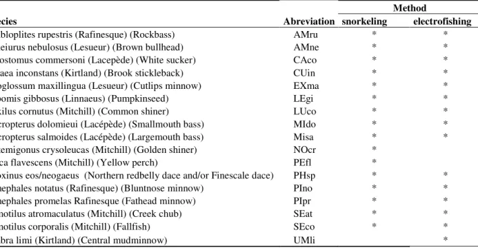
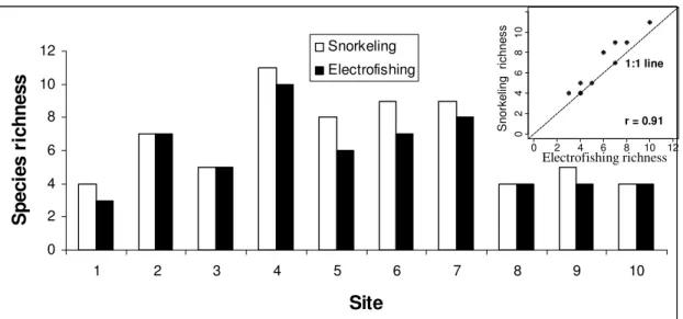
A total of 17 species belonging to 7 families were recorded during the field surveys (Table 2). Cyprinids (8 species) was the most represented family, accounting for an average of 75% of individuals per site, followed by Centrarchids (4 species), accounting for an average of 18% of the individuals (Table 1). Species richness ranged from 4 to 11 for snorkeling and from 3 to 10 for electrofishing (Figure 2). Electrofishing permitted to sample 15 species (all sites combined), but was unsuccessful at sampling golden shiner (Notemigonus crysoleucas) and yellow perch (Perca flavescens). Golden shiners were only present in low abundances (1 individual) in 2 sites and yellow perch were present in 4 sites, also in very low abundances (from 1 to 12 individuals per sites). In contrast, snorkeling surveys permitted the observation of a total of 16 species, but was inefficient at detecting the presence of central mudminnows (Umbra limi) at any of the sites.
Table 2 Species sampled, abbreviation and method with which the species was detected.
Method
Species Abreviation snorkeling electrofishing
Ambloplites rupestris (Rafinesque) (Rockbass) AMru * *
Ameiurus nebulosus (Lesueur) (Brown bullhead) AMne * *
Catostomus commersoni (Lacepède) (White sucker) CAco * *
Culaea inconstans (Kirtland) (Brook stickleback) CUin * *
Exoglossum maxillingua (Lesueur) (Cutlips minnow) EXma * *
Lepomis gibbosus (Linnaeus) (Pumpkinseed) LEgi * *
Luxilus cornutus (Mitchill) (Common shiner) LUco * *
Micropterus dolomieui (Lacépède) (Smallmouth bass) MIdo * * Micropterus salmoides (Lacépède) (Largemouth bass) Misa * * Notemigonus crysoleucas (Mitchill) (Golden shiner) NOcr *
Perca flavescens (Mitchill) (Yellow perch) PEfl *
Phoxinus eos/neogaeus (Northern redbelly dace and/or Finescale dace) PHsp * * Pimephales notatus (Rafinesque) (Bluntnose minnow) PIno * *
Pimephales promelas Rafinesque (Fathead minnow) PIpr * *
Semotilus atromaculatus (Mitchill) (Creek chub) SEat * *
Semotilus corporalis (Mitchill) (Fallfish) SEco * *
Fig. 2 Comparison of species richness observed by each sampling method at each site. Inset: graphical
representation of the relationship between snorkeling and electrofishing species richness. Pearson’s corrlelation was tested using 999 permutations (p=0.001).
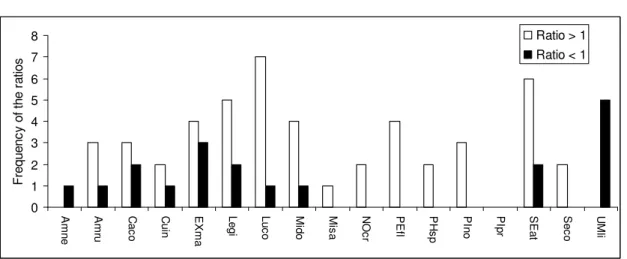
Total abundance of fish per 20 m long river section ranged from 9 to 313 fish for electrofishing and from 17 to 387 for snorkeling and fish of Size Class 1, on average, accounted for 18% (standard deviation (sd) = 18%) of total abundance for snorkeling and averaged 26% (sd = 32%) of electrofishing abundances. The Pearson’s correlation between the total abundances of fish observed by electrofishing and snorkeling was high both when fish belonging to Size Class 1 were included (r = 0.98, p = 0.001) or excluded (r = 0.99; p = 0.001) from the analysis (Figure 3). The correlations were tested using 999 permutations because the variables were not normally distributed. For most species, the average abundance per site was higher (from 0 to 26 more fish) for snorkeling than for electrofishing (Figure 4). The two exceptions in this respect were the brown bullhead (Ameiurus nebulosus) and the central mudminnow for which abundances were always higher (respectively 6 and 12 more fish, on average) for electrofishing than for snorkeling.
Sampling sites were characterized by average flow velocities ranging from 14 to 56 cm•s-1, relatively high water temperatures (range = 18 – 22°C) and low conductivity (range = 31.0 -91.9; Table 1). The sites were also characterized by a dominance of fine substrates (65% of the sites were covered by clay, silt and sand; Table 1). The first two axes of the
0 2 4 6 8 10 12 1 2 3 4 5 6 7 8 9 10 Site S p e c ie s r ic h n e s s Snorkeling Electrofishing 0 2 4 6 8 10 12 0 2 4 6 8 1 0 Electrofishing richness S n o rk e lin g ri c h n e s s r = 0.91 1:1 line
PCA represented most of the variation of the percent cover of the 7 substrate classes, with the first and second axes respectively representing 60.9 and 28.6% of the variation (Figure 5). The first axis was positively correlated with silt (r = 0.958; p = 2.881e-05) and negatively correlated with pebble (r = -0.872; p-value = 0.000981) and gravel (r = -0.742; p = 0.01388) while the second axis was positively correlated with sand (r = 0.966; p-value = 5.923e-06).
Fig. 3 Comparison of snorkeling total abundance and electrofishing estimated total abundance (a), and
snorkeling abundance and electrofishing estimated total abundance excluding fish of size class 1 (b). Pearson’s correlation coefficient are also shown
Forward selection based on snorkeling-derived estimates of abundance did not select for variables other than electrofishing total abundance (94.9% of the variance explained; Table 3). When using total abundance of fish observed by snorkeling excluding fish of Size Class 1, the forward selection selected electrofishing total abundance (excluding Size Class 1; 96.7% of the variance explained) and the first principal component of the PCA on the substrate classes (1.7% of the residual variance explained). The forward selection using the Hellinger distance between the fish communities observed by each sampling method as the response variable selected no explanatory variables at an alpha level of 0.05. 0 100 200 300 400 0 1 0 0 2 0 0 3 0 0 4 0 0
Electrofishing estimated abundance
S n o rk e lin g a b u n d a n c e (a) 1:1 line r = 0.98 0 50 100 150 200 250 300 0 5 0 1 0 0 1 5 0 2 0 0 2 5 0 3 0 0
Electrofishing estimated abundance
S n o rk e lin g a b u n d a n c e (b) 1:1 line r = 0.99
Fig. 4 Frequency of the ratio of abundances (snorkeling / electrofishing) for each
species. A ratio greater than 1 means more fish of a species were observed by snorkeling than electrofishing at a sampling site. The sum of the frequencies for each species is equal to the number of sites where they were detected by either sampling method, except for the following species, for which ratios equal to 1 were observed at 1 site: AMru, CUin, EXma, LUco, MIdo, PIpr and SEat
-5 0 5 10 -5 0 5 1 0 PC1 (60.9%) P C 2 ( 2 8 .6 % ) Clay Silt Sand Gravel Pebble Cobble Boulder
Fig. 5 Principal component analysis on the covariance matrix of the 7 substrate classes (percent cover),
scaling type 1. The first axis represents 60.9% of the variation and the second 28.6% 0 1 2 3 4 5 6 7 8 A m n e A m ru C a c o C u in E X m a L e g i L u c o M id o M is a N O c r P E fl P H s p P In o P Ip r S E a t S e c o U M li F re q u e n c y o f th e r a tio s Ratio > 1 Ratio < 1
Table 3: Cumulative adjusted r-square (R2
adj), regression coefficients, standart error, t- and p-value of the forward selection of explanatory variables on MLR using snorkeling total fish abundance, snorkeling total fish abundance excluding fish of Size Class 1 and the Hellinger distance between the fish communities sampled by each method at each site as the response variables
Response Parameters Coefficients
R2
adj Estimate Std.Error p-value
Snork. total fish abundance Intercept 0.0000 0.0945 1
Electro. estimated total abundance 0.949 0.9595 0.0996 1.1E-05 *** Snork. total fish abundance
(excluding fish of size class 1)
Intercept 0.0000 0.0405 1
Electro. estimated total abundance (excluding fish of size class 1)
0.967 1.0010 0.0430 6.90E-08 ***
PC1 (substrate) 0.984 -0.1293 0.0430 0.0198 *
Hellinger distance no variable selected NA NA NA NA
Discussion
The goals of this study were to evaluate the relative performance of electrofishing and snorkeling for estimating the abundance of fish species and size classes for non-salmonid communities and to assess the effect of environmental conditions on potential differences between the results obtained using these two methods. The results showed that the two sampling methods provided similar assessment of the fish communities but snorkeling observed greater species richness than electrofishing in most of the sites (6/10; Figure 2). We haven’t found any study comparing back-pack electrofishing and snorkeling for the assessment of species richness in communities with more than 3 species. However, Goldstein (1978) consistently observed more species (from 1 to 5, richness range: 9 - 18) using snorkeling than a comparable seining effort in Connecticut streams. In this study, the fish communities were dominated by catostomids, cyprinids and centrarchids (6 families represented), similarly to the ones in our study.
For most of the species (15/17), snorkeling observed more individuals per site than electrofishing (Figure 4). However, central mudminnows were never observed by snorkeling. Brind'Amour and Boisclair (2004) also failed to detect central mudminnows with visual surveys in a Laurentian lake. This species is known to burrow into the mud to escape predators (Scott and Crossman 1985), which could explain why daytime snorkeling surveys did not allow the survey of this species. The brown bullhead, observed in 1 site, was under sampled by snorkeling. This species is known to be more active at night (Scott and Crossman 1985) and we also observed it burrowed into the substrate during the daytime sampling, which could explain why more fish were electrofished than observed by snorkelers.
The correlation between electrofishing total abundance and snorkeling total abundance (Figure 3a) was high, as well as the correlation between total abundances excluding fish of Size Class 1, which could have been underestimated by electrofishing, as suggested by Reynolds (1996). 100% of the points of the relationships between electrofishing and snorkeling total abundance were above the 1:1 line, meaning that in all sites, snorkeling observed more fish than electrofishing. Snorkelers counting fish more than
once could have led to overestimation of fish abundances. However, snorkelers were rigorously trained (more than 2 months) and would never count fish escaping upstream, since they were going to be enumerated later (fish were confined in the sampling sites by the block nets). Moreover, the tendency of snorkeling surveys to observe more fish than electrofishing is consistent with the greater species richness observed in most of the sites during the snorkeling surveys. A number of studies also obtained good correlations between electrofishing and snorkeling abundances, like Hankin and Reeves (1988; r > 0.90) for 1+ coho salmon and 1+ steelhead trout, Wildman and Neumann (2003; 0.58 < r2 < 0.93) for brook and brown trouts, and Mullner et al. (1998; 0.90 < r2 < 0.99) for brook, cutthroat and rainbow trouts. However, in all these studies, the electrofishing abundances were higher than the snorkeling abundances.
Effect of abiotic conditions:
The second objective of this study was to evaluate if the environmental conditions could explain the potential differences between the fish communities observed by snorkeling and electrofishing. A forward selection of the explanatory variable using multiple linear regressions was used to model the 3 different response variables (snorkeling total abundance, snorkeling abundance excluding fish of Size Class 1 and the Hellinger distance between the fish communities observed by each sampling method; Table 3). The electrofishing abundance was found to explain most of the variation of the snorkeling total abundance. Likewise, when excluding fish of Size Class 1, the forward selection included the electrofishing total abundance (excluding Size Class 1) as the most important explanatory variables, but also selected the first principal component of the PCA performed on the 7 substrate classes. Yet, PC1 only explained 1.7% of the variation not explained by electrofishing estimates of total abundance. Finally, the forward selection using the Hellinger distance between the fish communities observed by each sampling method did not include any significant environmental characteristic, thus reinforcing the hypothesis that there is no environmental descriptor that could explain a biologically relevant portion of the differences between the fish communities described by the 2 sampling methods
among our sites. However, we are cautious to generalise our conclusions for the Laurentian streams since the sampling size was relatively small.
We do not think that the observed superiority of the snorkeling surveys is related to the low conductivity of our streams. First, this environmental descriptor was not found to be significantly related to the difference between snorkeling and electrofishing in any of the statistical models. We also visually observed the relationships to make sure there was no non-linear trend in the data. Second, it is difficult to compare our results with studies opposing snorkeling surveys and back-pack electrofishing (Table 4), because the only conductivity values mentioned were in Cunjak et al. (1988; 109 µsiemens) and Thurow and Schill (1996; 102 µsiemens), and did not vary within the study. Nonetheless, Peterson et al. (2004) found that stream characteristics were related to multipass electrofishing efficiency, but never found significant relationships with conductivity in streams where this descriptor varied from 16 to 203 µsiemens (mean = 58). Finally, many studies performed electrofishing surveys in low-conductivity streams (Kanno et al. 2009; Habera et al. 2010) and proper setting of voltage (to maintain power) should compensate for this drawback (Reynolds 1996).
Wildman and Neumann (2003) found that woody debris variables could improve the prediction of electrofishing depletion estimates based on snorkel counts. Mullner et al. (1998) reported that regression models predicting electrofishing depletion estimates from snorkel counts for three trout species were improved with the addition of visibility and instream cover variables (fallen trees, woody debris, large cobble, and boulders). Our sampling sites had different environmental characteristics from those observed in the 2 previous studies (no fallen trees, insignificant cover of large cobble and boulders, the most important instream cover descriptor being aquatic plants), but the most striking dissimilarity is between the fish communities observed.
Effect of biotic descriptors of fish communities:
Our study is different from the others since the comparison between back-pack electrofishing and snorkeling surveys was carried out in streams dominated by cyprinids and centrarchids, as opposed to salmonid dominated streams (Table 4), while the environmental conditions were suitable for both methods. Vulnerability to electrofishing varies according to the species sampled (Reynolds 1996) and a few studies reported that cyprinids and centrarchids had lower electrofishing capture efficiencies than other families. For instance, Meador et al. (2003) mentioned that cyprinids and centrarchids were the 2 most likely families (among the 7 most common) to be missed on the first electrofishing pass. Bayley and Dowling (1990) obtained very low capture efficiency with electrofishing for cyprinids (< 0.25), and Kimmel and Argent (2006) observed that small percids (e.g., darters) and schooling fish (e.g., cyprinids) avoided capture more frequently than other common families. Also, Reynolds (1996) mentioned that salmonids tend to be more vulnerable to electroshocking than cyprinids.
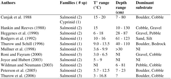
Table 4: Previous studies comparing snorkeling surveys with electrofishing (NI = not identified in the
reference)
Authors Families ( # sp) T° range
(°C) Depth range (cm)
Dominant substrate
Cunjak et al. 1988 Salmonid (2) Cyprinid (1)
15 - 20 7 - 80 Boulder, Cobble Hankin and Reeves (1988) Salmonid (2) 15 10 - 130 Cobble, Gravel Heggenes et al. (1990) Salmonid (2) 6 - 18 28 - 87 Gravel, Pebble Rodgers et al. (1992) Salmonid (1) 10 - 16 61 - 123 Sand, Silt Thurow and Schill (1996) Salmonid (1) 9.0 - 13.5 40 - 110 Boulder, Bedrock Mullner et al. (1998) Salmonid (3) 3.6 - 9.9 >30 NI
Roni and Fayram (2000) Salmonid (3) 3.0 - 6.5 NI Gravel, Cobble Joyce and Hubert (2003) Salmonid (2) 5 – 9 NI NI
Wildman and Neumann (2003) Salmonid (2) NI 6 - 81 Pebble, Cobble Peterson et al. (2005) Salmonid (2) 5.7 - 12.5 7 - 23 Boulder, Cobble Thurow et al. (2006) Salmonid (3) 3 - 16.8 ? Boulder, Cobble
The lack of relationship between the differences in the fish communities observed by the 2 sampling methods and environmental conditions in our study could be explained
by the behaviour of the fish encountered. Salmonids may show territorial and cryptic behaviours (Thurow and Schill 1996; Peterson et al. 2004), which could explain why the inclusion of habitat complexity descriptors can help predict the electrofishing depletion estimates based on snorkeling surveys (Mullner et al. 1998; Peterson et al. 2004; Wildman and Neumann 2003). Cyprinids and centrarchids do not tend to show these types of behaviours (except for territoriality during reproduction, particularly for Centrarchids from May to mid-July; Moyle and Cech 2004), but tend to show schooling behaviours (Kimmel and Argent 2006; McCartt et al. 1997). Schooling fish may show group fright response and evade capture more frequently than non-schooling species (Kimmel and Argent 2006; Reynolds 1996). It may also be more difficult to capture all fish from a school using electrofishing than for snorkelers to estimate the abundance of fish in such schools. We also frequently observed centrarchids remaining stationary and facing the snorkeler. This behaviour, also reported by Goldstein (1978), could facilitate the snorkeling counts.
In conclusion, electrofishing and snorkeling surveys were found to be two complementary methods for sampling fish communities in the lower Laurentian streams. Snorkeling, however, observed more fish species in six of the ten sites and higher abundances in all of the sampling sites. Snorkeling also allowed for a more cost-effective enumeration of species and abundances since the same sampling units could be surveyed in a fifth of the time needed to conduct 3 pass depletion electrofishing. Our results also suggest that, in some streams where the environmental conditions are suitable for both sampling methods, fish communities may be more important than environmental descriptors at determining the efficiency of snorkeling surveys relative to back-pack electrofishing. Finally, we would like to remind that snorkeling efficiency highly relies on the field assistants’ expertise and that proper training is a key element for the success of such field surveys.
Aknowledgements
We thank Guillaume Bourque, Florian Bonnaire, Jérémie Vernay and Yohan Fittere for their field assistance. Financial support was provided by Fond Québécois pour la Recherche sur la Nature et les Technologies (FQRNT) and the Natural Sciences and Engineering Research Council of Canada (NSERC).
28
Comparison among different fish functional
classification methods to develop habitat use
models
Jean-Martin Chamberland and Daniel Boisclair
Université de Montréal, Département de sciences biologiques, C.P. 6128, Succursale
Centre-ville, Montréal, Québec, Canada H3C 3J7
Contribution to the programme of GRIL (Groupe de Recherche Interuniversitaire en Limnologie et en environnement aquatique).
29
Abstract
Fish habitat use models (FHUM) are quantitative relationships between biological descriptors of fish (biomass, abundance, density) and environmental descriptors (depth, flow velocity, substrate type, etc.). In species rich communities, developing FHUM for every species and ontogenetic stage can be quite challenging. In order to simplify the modelling of such communities, as well as improve our understanding of fish – habitat relationships, we used the ecological guild concept and the niche filtering hypothesis to explore the relationships between guilds based on different types of traits (eco-morphological, reproductive, alimentary and taxonomic) and local environmental descriptors, at the coarse meso-habitat scale. Reproductive guilds led to FHUM that clearly outperformed the other 3 approaches, because of the close relationship between preferred spawning grounds and non spawning habitat preferences, and also because reproductive traits are linked to habitat characteristics at the reach or coarse mesohabitat scale. We also defined guilds based on habitat-use and related them to species traits. Traits related to the feeding biology of fishes seemed to be the best at explaining the habitat-use guilds, but our model did not correctly represent the among-guild relationships. Validation of our reproductive trait model on an independent dataset would confirm our finding, which represents a promising way of modelling fish - habitat relationships in complex fish communities.
Keywords : Fish habitat use models, centrarchid, cyprinid, guild, reproductive, alimentary, eco-morphological and taxonomic traits, stream, meso-habitat