The Importance of the Loss Function in Option Pricing

(1)

Série Scientifique

Scientific Series

2001s-45

The Importance of the Loss

Function in Option Pricing

(2)

CIRANO

Le CIRANO est un organisme sans but lucratif constitué en vertu de la Loi des compagnies du Québec. Le financement de son infrastructure et de ses activités de recherche provient des cotisations de ses organisations-membres, d’une subvention d’infrastructure du ministère de la Recherche, de la Science et de la Technologie, de même que des subventions et mandats obtenus par ses équipes de recherche.

CIRANO is a private non-profit organization incorporated under the Québec Companies Act. Its infrastructure and research activities are funded through fees paid by member organizations, an infrastructure grant from the Ministère de la Recherche, de la Science et de la Technologie, and grants and research mandates obtained by its research teams.

Les organisations-partenaires / The Partner Organizations •École des Hautes Études Commerciales

•École Polytechnique •Université Concordia •Université de Montréal

•Université du Québec à Montréal •Université Laval

•Université McGill

•Ministère des Finances du Québec •MRST

•Alcan inc. •AXA Canada •Banque du Canada

•Banque Laurentienne du Canada •Banque Nationale du Canada •Banque Royale du Canada •Bell Québec

•Bombardier •Bourse de Montréal

•Développement des ressources humaines Canada (DRHC) •Fédération des caisses Desjardins du Québec

•Hydro-Québec •Industrie Canada

•Pratt & Whitney Canada Inc. •Raymond Chabot Grant Thornton •Ville de Montréal

Short sections may be quoted without explicit permission, if full credit, including © notice, is given to the source.

ISSN 1198-8177

Ce document est publié dans l’intention de rendre accessibles les résultats préliminaires de la recherche effectuée au CIRANO, afin de susciter des échanges et des suggestions. Les idées et les opinions émises sont sous l’unique responsabilité des auteurs, et ne représentent pas nécessairement les positions du CIRANO ou de ses partenaires.

This paper presents preliminary research carried out at CIRANO and aims at encouraging discussion and comment. The observations and viewpoints expressed are the sole responsibility of the authors. They do not necessarily represent positions of CIRANO or its partners.

(3)

The Importance of the Loss Function in Option Pricing

*

Peter Christoffersen

†

, Kris Jacobs

†

Résumé / Abstract

Quelle fonction de pertes devrait être utilisée pour l'estimation et l'évaluation des modèles d'évaluation d'options? Plusieurs fonctions différentes ont été suggérées, mais aucune norme ne s'est imposée. Nous ne promouvons aucune fonction, mais soutenons que la cohérence dans le choix des fonctions est cruciale. Premièrement, pour n'importe quel modèle donné, la fonction de pertes utilisée dans l'estimation des paramètres et dans l'évaluation du modèle devrait être la même, sinon on obtient des estimations de paramètres sous-optimales. Deuxièmement, lors de la comparaison de modèles, la fonction de pertes pour l'estimation devrait être la même pour chaque modèle, autrement les comparaisons sont injustes. Nous illustrons l'importance de ces questions dans une application du modèle appelé Black-Scholes du praticien (PBS) aux options de l'index S&P500. Nous trouvons des réductions de plus de 50 pourcent de la racine de l'erreur quadratique moyenne du modèle PBS lorsque les fonctions de pertes d'estimation et d'évaluation sont alignées. Nous trouvons également que le modèle PBS dépasse un modèle de benchmark structurel quand les fonctions de pertes d'estimation sont identiques pour tous les modèles, mais pas dans les autres cas. Le nouveau modèle PBS à fonctions de pertes alignées représente dès lors un benchmark bien plus robuste auquel les futurs modèles structurels pourront être comparés.

Which loss function should be used when estimating and evaluating option pricing models? Many different fucntions have been suggested, but no standard has emerged. We do not promote a partidular function, but instead emphasize that consistency in the choice of loss functions is crucial. First, for any given model, the loss function used in parameter estimation and model evaluation should be identical, otherwise suboptimal parameter estimates will be obtained. Second, when comparing models, the estimation loss function should be identical across models, otherwise unfair comparisons will be made. We illustrate the importance of these issues in an application of the so-called Practitioner Black-Scholes (PBS) model to S&P500 index options. We find reductions of over 50 percent in the root mean squared error of the PBS model when the estimation and evaluation loss functions are aligned. We also find that the PBS model outperforms a benchmark

*_{Correspondence to: Peter Christoffersen, Fac. of Management, McGill University, 1001 Sherbrooke St. West,}

Montréal, Qc, Canada H3A 1G5 Tel: (514) 398-2869 Fax: (514) 398-3876 email: christop@management.mcgill.ca We would like to thank Torben Andersen, Tim Bollerslev, Jérôme Detemple, Jin Duan, Nour Meddahi and the participants of the May 2001 CRDE conference on "Modelling, Estimating and Forecasting Volatility" and the June 2001 CIRANO conference on "Financial Mathematics and Econometrics" for helpful comments. We would also like

(4)

structural model when the estimation loss functions are identical across models, but otherwise not. The new PBS model with aligned loss functions thus represents a much tougher benchmark against which future structural models can be compared.

Mots Clés : Évaluation des options, volatilité implicite, approche Black-Scholes du praticien, erreurs d'évaluation, fonctions de perte, prévisions hors-échantillon, stabilité des paramètres

Keywords: Option pricing, implied volatility, practitioner Black-Scholes approach, pricing errors, loss functions, out-of-sample forecasting, parameter stability

(5)

1 Introduction

The literature on option pricing models has expanded dramatically over the last decade. A large number of models have been proposed to address the empirical shortcomings of the classic Black-Scholes (BS) (1973) approach. For instance, an important class of option pricing models speci¯es the volatility of the underlying asset as a deterministic function of time and the price of the underlying asset (see Derman and Kani (1994), Dupire (1994) and Rubinstein (1994)). Other studies have investigated stochastic volatility models (e.g. see Scott (1987), Hull and White (1987), Heston (1993) and Melino and Turnbull (1990)), jump models (Bates (1996a)) and discrete-time GARCH models (see Duan (1995) and Heston and Nandi (2000)).1

The objective of this paper is to contribute to the methodological debate on the estimation and evaluation of these models. A central theme of our work is that all models are to some degree misspeci¯ed. The recognition of model misspeci¯cation brings to center stage the choice of loss function in model estimation and evaluation. Most standard statistical estimation techniques assume that the model under consideration is correctly speci¯ed but simply contains a set of unknown parameters. In this case, most estimators will produce consistent estimates and thus yield the \true" parameter value if a large enough sample is at hand. The choice of estimation technique then largely boils down to ¯nding the most e±cient estimator under the prevailing conditions.

However, once model misspeci¯cation is recognized, the standard consistency result no longer applies: The parameter estimates obtained will depend on the choice of loss function, even as the sample gets in¯nitely large. There is no such thing as convergence to the \true" parameter value. Under this scenario, it is crucial to choose a loss function which is relevant for the purpose at hand.

The choice of loss function is particularly important in option pricing. Option pricing models are rarely estimated in order to draw inference about a structural parameter of in-trinsic interest. Rather, option pricing models are typically estimated for use in the pricing or hedging of traded options out-of-sample. Thus di®erent purposes, for example hedging, speculating or market making, imply di®erent loss functions on the model errors. Further-more, option pricing models tend to be based on relatively tightly parameterized models of the underlying asset dynamics and the price of risk, and under the assumption of frictionless markets. These simplifying assumptions have the important bene¯t of yielding closed-form option pricing formulae, but they quite possibly come at the cost of model misspeci¯cation. The multiple potential uses of option pricing models, and the possibility of misspeci¯cation, render the choice of loss function crucial.

The academic literature has not been oblivious to the importance of loss functions, but the

1_{For a more complete overview of di®erent approaches used in option pricing see Bakshi, Cao and Chen}

(6)

choice of loss function is typically based on statistical and numerical, rather than economic criteria. Whereas some papers in the literature use a loss function based on implied volatility, others calibrate and estimate their models using loss functions based on squared dollar pricing errors (e.g. see Heston and Nandi (2000), Bakshi, Cao and Chen (1997)), relative pricing errors, or a likelihood-based approach (Jacquier and Jarrow (2000)). We do not promote a particular loss function as the choice depends on the end-use of the model, but instead we emphasize that consistency in the choice of loss functions is crucial. Our contribution in this regard is threefold:

First, for any given model, we demonstrate that the loss function used in parameter estimation and model evaluation must be identical in order to minimize the evaluation loss. If the model under consideration is the \true" model then asymptotically any well-behaved loss function will yield the \true" parameter values which in turn will minimize all loss functions. But in a more realistic case where the model is misspeci¯ed, the loss function issue is key. We illustrate the importance of the loss function in an application of the benchmark Dumas, Fleming and Whaley (1998) (DFW) implied volatility model, which they refer to as the Practitioner Black Scholes (PBS) model. Using three years of European options on the S&P500 index, we show that correctly aligning the estimation and evaluation loss functions can yield improvements of over 50 percent in the evaluation loss.

Second, when comparing models, the estimation loss function should be identical across models, otherwise unfair comparisons will be made. The PBS model is typically implemented using an implied volatility loss function, which conveniently yields a linear estimator of the parameters. Implemented this way, the PBS model is easily outperformed by more structural stochastic volatility or GARCH option pricing models which are implemented with an estimation loss function which more closely matches the evaluation loss. But our empirical study shows that when the PBS model is implemented fairly, that is, by using the same estimation loss function as the structural model, the PBS model actually outperforms the structural model both in- and out-of-sample.

Third, by implementing the PBS model fairly, we introduce a new PBS model with aligned loss functions, which performs much better than the old. This modi¯ed PBS model represents a tougher benchmark against which future structural models can be compared.

The paper proceeds as follows. In Section 2, we ¯rst discuss the di®erent loss functions used in empirical option pricing, and we give an overview of their use in the literature. We then present the Practitioner Black-Scholes approach as implemented by DFW and our modi¯cation of their approach. Finally, we brie°y summarize the relevant theoretical results on estimation under di®erent loss functions. Section 3 describes the data, Section 4 presents our empirical results, and Section 5 brie°y discusses the Heston (1993) model and compares it with the PBS model. Section 6 concludes.

(7)

2 Methodology

The choice of loss function is particularly important in option pricing. Option pricing models are typically estimated for use in the pricing or hedging of options out-of-sample. Thus dif-ferent purposes, for example hedging, speculating or market making, might imply di®erent loss functions on the model errors. Even when attention is restricted to simple statistical loss functions, the issue of aligning the evaluation and estimation loss function is key. How-ever, in the extensive and growing literature on option pricing, the speci¯cation of the loss function has until now not received much attention compared to other issues, such as model speci¯cation and the estimation of continuous-time processes underlying option models. For example, the excellent overview in Campbell, Lo and MacKinlay (1997) does not list any contributions on the importance of the selection of the loss function.

The use of di®erent loss functions at the estimation and evaluation stage is generally accepted and widely used in the literature. For example, Bakshi, Cao and Chen (1997) use $M SE in estimation and %M SE as well as $M SE in the evaluation stage. Rosenberg and Engle (2000) use $M SE in estimation, and % hedging error in evaluation. Hutchinson, Lo and Poggio (1994) use an MSE based on option price divided by exercise price, and evaluate the model out-of-sample using hedging errors, among other things. Also, several papers estimate model parameters from option prices using an estimation loss function based on the statistical properties of the underlying process or the statistical structure of the measurement errors (see Renault (1997), Jacquier and Jarrow (2000)) and proceed to evaluate the models out-of-sample using a di®erent loss function. Pan (2000) uses a GMM loss function in estimation and IV MSE in evaluation. Chernov and Ghysels (2000) estimate parameters using EMM, and evaluate models using $MSE and %M SE loss functions. Benzoni (1998) estimates parameters using both EMM and $M SE (normalized by the index value) and proceeds to evaluate the model using $MSE (again normalized). Finally, whereas most recent papers estimate option pricing parameters using option data or option data as well as returns data, until recently many option pricing studies were conducted by estimating option pricing parameters from asset returns and inserting these parameters in option pricing formulae out-of-sample. Again, this amounts to using a di®erent loss function in-sample and out-of-sample.

Problems may arise when one compares out-of-sample errors generated in this way with the errors from other models where in-sample and out-of sample loss functions are identical. For example, DFW (1998) compare the out-of-sample performance of the PBS model with the out-of-sample performance of the implied tree models implemented with identical in-and out-of-sample loss functions. The conclusion of DFW is that the pricing performance of the PBS model compares favorably with that of the implied tree models. Because the implementation of the PBS model proposed in this paper will certainly not deteriorate the model's performance, the conclusions of DFW will therefore be reinforced when the PBS model is implemented properly. This may not be the case for the studies by Heston and

(8)

Nandi (2000) and Garcia, Luger and Renault (2000). Both papers use the $M SE loss functions for the out-of-sample comparison, but use the implied-volatility based loss function for the PBS model in estimation. Heston and Nandi (2000) then compare the PBS model with a GARCH model which has identical in-sample and out-of-sample loss functions. They ¯nd that the GARCH model improves upon the performance of the PBS model. Garcia, Luger and Renault (2000) compare PBS to a new Generalized Black-Scholes model, which is also implemented with aligned loss functions, and which is also found to dominate the PBS model. The potential problem is that both studies use the PBS model as a benchmark, but the performance of the benchmark is not as good as it would be if it were implemented using the appropriate loss function.

We now proceed to analyze impact of the loss function in more detail. First, we describe the loss functions most commonly used to estimate and calibrate parameters in empirical option pricing. Then we introduce the PBS model which can be viewed as an ad-hoc model of the well-known \smile" and \smirk" patterns exhibited by standard derivatives prices. We also discuss relevant results from the econometrics literature on the estimation of misspeci¯ed models, which in turn motivates the ensuing empirical study.

2.1 Option Pricing Model Evaluation

The performance of di®erent option pricing models is often evaluated using mean-squared dollar errors, that is, the loss function is given by

$M SE(µ) = 1 n n X i=1 (Ci¡ Ci(µ))2 (1)

where Ci and Ci(µ) are the data and model option prices respectively, and n is the number of option contracts used.2 The $M SE loss function has the advantage that the errors are easily interpreted as $-errors once the square root is taken of the mean-squared-error. However, the relatively wide range of option prices across moneyness and maturity raises the problem of heteroskedasticity for $M SE-based parameter estimation.

Also, because the $M SE loss function implicitly assigns a lot of weight to options with high valuations (in-the-money and long time-to-maturity contracts) and therefore high $-errors, some researchers instead favor the relative or percent loss function,3 _{de¯ned as}

%M SE(µ) = 1 n n X i=1 ((Ci¡ Ci(µ))=Ci)2 (2)

2_{Although we estimate new parameters each day, we omit the time subscript, t, on the parameters in this}

section in order to save on notation.

3_{Note that the %-sign below is just a convenient short-hand for relative loss. We do not in fact multiply}

(9)

The %M SE loss function has the advantage that a $1 error on a $50 dollar option carries less weight than a $1 error on a $5 option, which is sensible from a rate-of-return perspective. The disadvantage is that short-time to maturity out-of-the money options with valuations close to zero will implicitly get assigned a lot of weight and can create numerical instability if the %MSE loss function is used in estimation.

Partly based on the above considerations of heteroskedasticity, and partly based on the market convention of quoting option prices in terms of volatility, some researchers favor estimating option pricing models minimizing the MSE of the implied Black-Scholes volatility from the option. We therefore de¯ne the implied volatility MSE as

IV M SE(µ) = 1 n n X i=1 (¾i¡ ¾i(µ))2; (3)

where the implied volatilities are obtained as

¾i = BS¡1(CiMkt; Ti; Xi; S; r); and ¾i(µ) = BS¡1(Ci(µ); Ti; Xi; S; r); (4) with BS¡1 being the inverse of the Black-Scholes formula, CMkt

i the market price of option i, Ci(µ) the model price for option i, Ti the time-to-maturity, Xi the strike price, S the price of the underlying stock and r the riskless interest rate.

This paper only considers the loss functions in (1), (2) and (3). A number of other estimation loss functions are used in the literature as discussed above. Functions based on hedging or speculation loss could potentially be more interesting, but we focus on the three functions listed here as they are arguably the most prevalent in previous work.

2.2 The Practitioner Black-Scholes Model

We illustrate the importance of the estimation loss function using the simplest model pos-sible, namely the so-called Practitioner Black-Scholes (PBS) model. In the PBS model, implementation is done in three steps. First the Black-Scholes implied volatility is calcu-lated for each observed option. Second, the implied volatilities are regressed on di®erent polynomials in T and X using simple ordinary least squares. Third, the ¯tted values for volatility are plugged back into the Black-Scholes formula to get the practitioner model price. DFW consider di®erent implied volatility functions. We limit our attention to the most general model they investigate, which is of the form,4

¾ = µ0+ µ1X + µ2X2+ µ3T + µ4T2+ µ5XT + " (5)

4_{DFW consider switching between speci¯cations based on the number of maturities available in their}

data set on any given day. Our data set is su±ciently rich that the speci¯cation used in (5) would always be chosen by DFW's switching model.

(10)

and where the ¯tted value of the implied volatility is then

¾(µ) = µ0+ µ1X + µ2X2+ µ3T + µ4T2+ µ5XT (6) Notice that estimating (5) by OLS amounts to letting the estimation loss function be IV M SE. OLS solves

µIV = Arg min

µ IV M SE(µ)´ Arg minµ 1 n n X i=1 (¾i¡ ¾i(µ))2 = (Z0Z)¡1Z0¾ (7) where Z =h 1 X X2 _{T T}2 _XT i_{is the matrix of regressors from the implied volatility} model. To evaluate the model, the estimate of the parameter vector, µIV, is then plugged back into the implied volatility model, which in turn is plugged into the Black-Scholes formula. The model is typically assessed using

$M SE(µIV) = 1 n n X i=1 ³ Ci¡ CiBS(¾i(µIV)) ´2 (8) or %M SE(µIV) = 1 n n X i=1 ³³ Ci¡ CiBS(¾i(µIV)) ´ =Ci ´2 (9) In this framework, the estimation loss function, which is de¯ned on implied volatilities, is di®erent from the evaluation loss function, which is de¯ned on dollar or percent pricing errors. Whereas this is a convenient and easily implemented procedure, it has potentially serious costs if the model is assessed in terms of a $M SE or %M SE loss function as we shall see below. The appropriate procedure is instead to use nonlinear least squares (NLS) to directly estimate µ; as follows

µ$ = Arg min $M SE(µ)´ Arg min µ 1 n n X i=1 ³ Ci¡ CiBS(¾i(µ)) ´2 (10) or

µ%= Arg min %M SE(µ) ´ Arg min µ 1 n n X i=1 ³³ Ci ¡ CiBS(¾i(µ)) ´ =Ci ´2 (11) This approach amounts to estimating the model parameters using the relevant loss func-tion. Baring potential numerical problems in the nonlinear estimation, this should generate better in-sample ¯t. The key question is how the di®erent estimates fare out-of-sample, which will be assessed below.

(11)

2.3 Parameter Estimation

As the three loss functions above are all well-behaved, and as the Black-Scholes pricing formula and the implied volatility function are continuous in the parameters, the estimates will in each case asymptotically converge to the values which minimize the estimation loss function. More explicitly, in population, let

µX¤ = Arg min

µ nlim!1XM SE(µ); for X = $; %; IV (12) Then, as the Black-Scholes pricing function is continuous in the parameter vector, µ, and using the results in White (1981), we get

lim

n!1µX = µ ¤

X; (13)

where, depending on the loss function, µX is either µIV; µ$ or µ%, that is, the loss-function speci¯c, ¯nite sample estimates from above.5

Notice that we can view µ% as a weighted least squares (WLS) estimate of µ$ and vice versa, where the weights are 1=C2

i and Ci2 respectively.6 Under the general assumption that the model being estimated is misspeci¯ed, White (1981) shows that the WLS estimate will converge to a limit which depends on the weights, and which will therefore be di®erent from the unweighted least squares estimate.7 _{As we are estimating the practitioner version} of the Black-Scholes model, which clearly violates the underlying assumption of constant volatility, model misspeci¯cation is indeed built-in from the start. Furthermore, it is probably reasonable to assume that the tightly parameterized structural models put forth in the literature are all to some degree misspeci¯ed, but the quantitative importance of this from a loss function perspective is of course an empirical question.

For our purposes, it su±ces to notice that as the implied volatility function estimated is clearly misspeci¯ed, the estimates from each loss function will converge to di®erent limits, that is

µ_IV¤ _{6= µ}_$¤ _{6= µ}¤_% (14)

Thus even asymptotically, the estimates minimizing IV M SE will not minimize $M SE etc. Consequently, under the realistic assumption that the model is misspeci¯ed, matching the estimation loss function to the evaluation loss function will matter{even asymptotically. How important this is in a realistic ¯nite-sample, out-of-sample setting will be the focus of the empirical analysis below.

5_{Thus µ}

IV is from an OLS regression, and µ$ and µ%are from NLS estimation.

6_{Note that the loss functions mentioned above which normalize the option pricing error by the strike}

price or the stock price can be viewed as WLS estimates of the $MSE loss as well.

7_{Thus we could construct tests for model misspeci¯cation based on the di®erences between µ}

% and µ$.

(12)

We close this section by noting that we are not promoting any particular loss function but instead stressing the importance of being consistent in the choice of loss function when the model is potentially misspeci¯ed. In order to obtain the best possible ¯t, the loss function used in out-of-sample evaluation should also be used in in-sample estimation. If a researcher is interested in several di®erent loss functions when evaluating and comparing models, care should be taken that the estimation loss function is identical across models, otherwise unfair comparisons will be made.

3 The Data

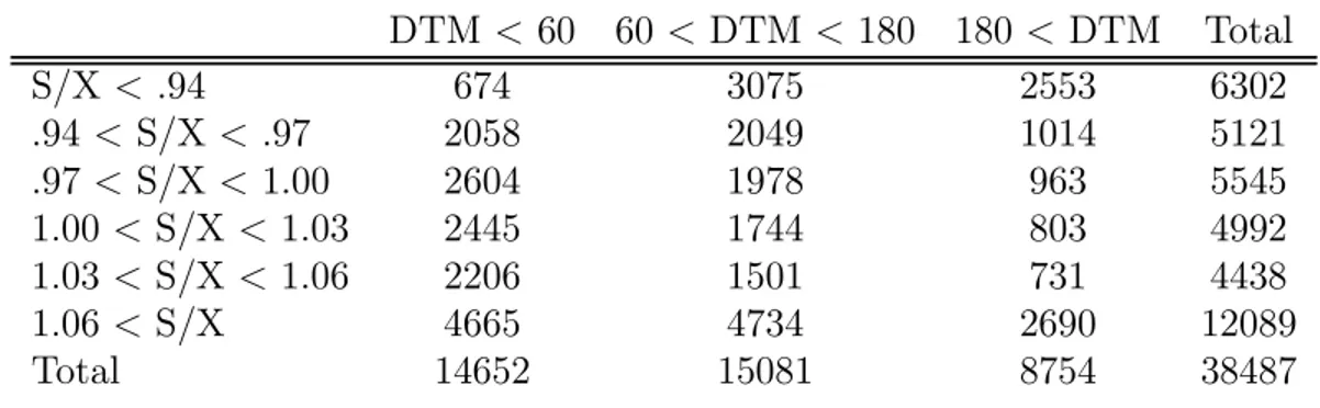
We analyze the methodological issues outlined above using a very standard data set on S&P 500 call option prices for 755 days in the period from June 1, 1988 through May 31, 1991. The data were graciously provided to us by Gurdip Bakshi and are practically identical to the ones used in the Bakshi, Cao and Chen (1997) study. We limit ourselves to a few important features of the data here and refer the reader to that study for further details. The data set is well suited for our empirical analysis because options written on the S&P 500 are the most actively traded European style contracts. Particular care was taken to adjust the S&P 500 spot index series for dividend payments and to obtain synchronous recording of stock and option prices. The resulting data set contains a wide variety of option quotes for di®erent values of moneyness and maturity. Table 1 lists the number of contracts for a set of maturity and moneyness bins, where S=X denotes the option's moneyness and DT M stands for days to maturity.8

Table 1: Number of Contracts Across Moneyness and Maturity DTM < 60 60 < DTM < 180 180 < DTM Total S/X < .94 674 3075 2553 6302 .94 < S/X < .97 2058 2049 1014 5121 .97 < S/X < 1.00 2604 1978 963 5545 1.00 < S/X < 1.03 2445 1744 803 4992 1.03 < S/X < 1.06 2206 1501 731 4438 1.06 < S/X 4665 4734 2690 12089 Total 14652 15081 8754 38487

Table 2A reports the average price for option contracts with di®erent moneyness and ma-turity. For our purpose, the most important observation in Table 2A is the large di®erences

8_{To be exact, we are sorting the data by (S}_¡D

i)=Xi; where Diis the present value of dividends accruing

(13)

in option prices for di®erent maturities and moneyness. As a result, expensive contracts would implicitly receive much more weight in the $M SE loss function than cheap contracts.

Table 2A: Average Call Prices Across Moneyness and Maturity DTM < 60 60 < DTM < 180 180 < DTM S/X < .94 1.53 5.09 10.32 .94 < S/X < .97 2.60 9.58 18.81 .97 < S/X < 1.00 5.29 14.87 25.00 1.00 < S/X < 1.03 11.02 21.25 31.32 1.03 < S/X < 1.06 18.44 28.06 37.19 1.06 < S/X 39.59 49.85 62.41

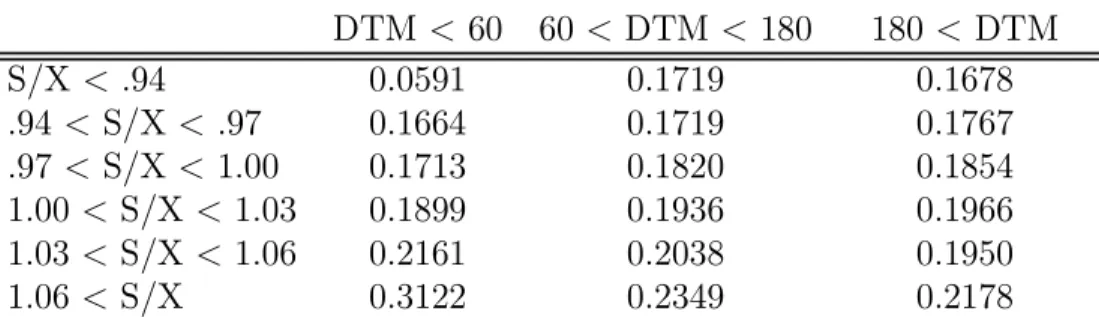
In Table 2B we report the average implied Black-Scholes volatilities from the call prices in Table 2A. Notice that in general the implied volatilities are much less variable across entries in the table than are the call prices themselves. A noticeable exception is the short-maturity, deep out of the money calls. Notice also that the well known post-crash smirk is apparent in every column, but that it is most apparent at the shortest maturity.

Table 2B: Average Implied Volatility Across Moneyness and Maturity DTM < 60 60 < DTM < 180 180 < DTM S/X < .94 0.0591 0.1719 0.1678 .94 < S/X < .97 0.1664 0.1719 0.1767 .97 < S/X < 1.00 0.1713 0.1820 0.1854 1.00 < S/X < 1.03 0.1899 0.1936 0.1966 1.03 < S/X < 1.06 0.2161 0.2038 0.1950 1.06 < S/X 0.3122 0.2349 0.2178

As mentioned above, we investigate the importance of the choice of loss function by estimating the relevant parameters for every one of the 755 daily cross sections. Figure 1 indicates that the optimization problem under study can be substantially di®erent for dif-ferent days. To illustrate the variation over the sample, we depict the average Black-Scholes implied volatility calculated for each of the 755 days in the sample. Notice that implied volatility changes through time but that swings in average implied volatility seem relatively persistent through time. This ¯nding suggests that the out-of-sample performance of some models may actually turn out to be fairly satisfactory if the parameters are appropriately estimated.

(14)

4 Empirical Results

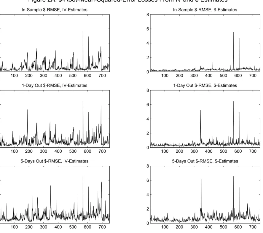
The main results of the paper are contained in Figures 2A and 2B and Table 3A. For each of the 755 days in the sample, we repeat the following exercise: First, we estimate the parameter µ characterizing the implied volatility function (5) using three di®erent loss functions. We will refer to these three estimates of µ as µt;$; µt;%and µt;IV respectively, where the t subscript indicates that the estimate was obtained using the t-th day (or cross-section) in the sample. The ¯rst estimate, µt;$; is obtained by minimizing the loss function (10). The second estimate, µt;%; is obtained by minimizing the loss function (11). The third estimate, µt;IV; is obtained by minimizing the loss function (7). Subsequently we use these estimates to evaluate the model's pricing performance in- and out-of-sample using di®erent loss functions.9 Possibly the most interesting exercise is to evaluate the di®erent loss functions one day out of sample. Consider the two middle pictures in Figure 2A. Both pictures show the square root of MSE's (RMSE) for the dollar-based loss function (1) evaluated at t + 1 using a parameter estimate obtained at t. However, in the left panel the estimate used is µt;IV , which is obtained by minimizing the \wrong" loss function (7). In contrast, in the right panel the estimate µt;$ is obtained by minimizing the \correct" loss function (10). The di®erences in RMSE between the two panels are striking. Whereas on a few occasions (especially in the second half of the sample) the RMSE is quite large in the right panel, the RMSE is often minuscule compared to the left panel.

The other panels in Figure 2A contain results for related exercises. In the two top panels we present the same exercise using estimates µt;IV and µt;$, but now the RMSE is computed for the same day t: Again we observe that the RMSE in the left panel is much larger than the RMSE in the right panel.10 _{Finally, the two bottom panels again use the estimates µ}

t;IV and µt;$, but now the RMSE is evaluated at day t+5. We see that whereas RMSEs in the left panel are not much di®erent from the ones in the top left panel, the RMSEs for the bottom right panel are considerably higher than the ones for the top right panel. Nevertheless, it is clear that the RMSEs in the bottom right panel are again much lower than those in the bottom left panel.

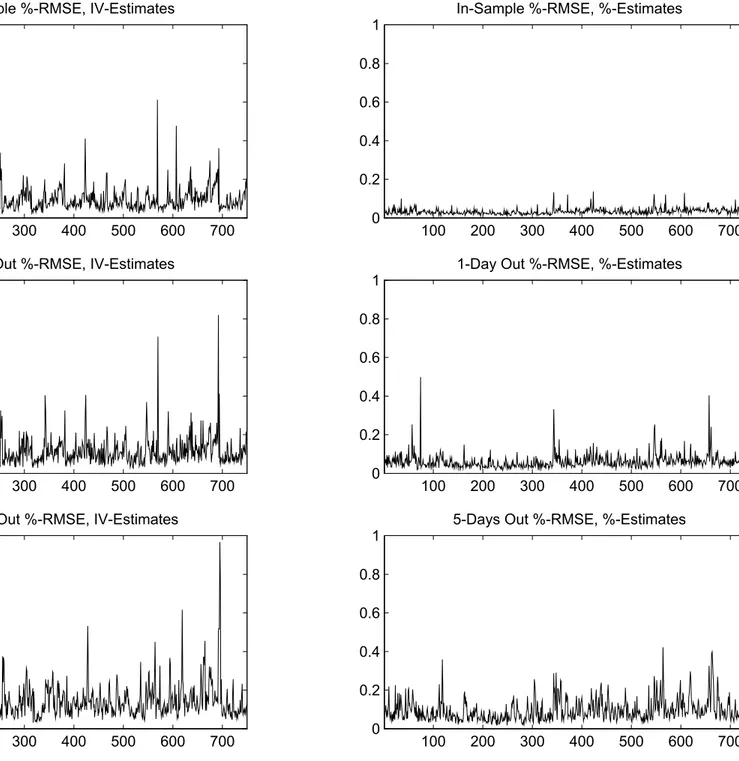
Figure 2B presents results for an exercise that is analogous to the one presented in Figure 2A, except that the RMSEs are now for the percentage-based loss function (2) evaluated at t, t + 1 and t + 5: The estimates used are the ones using the \wrong" loss function µt;IV and

9_{Our exercise is similar to Dumas, Fleming and Whaley (1998). Hull and Suo (2000) alternatively}

investigate the usefulness of the PBS model ¯tted to standard European options in-sample for pricing exotic options out-of-sample.

10_{The fact that the in-sample losses are so di®erent indicates the degree of misspeci¯cation of the model.}

If we were working with the true model, then asymptotically the parameters would be identical across loss functions, and the in-sample losses would therefore be the same across loss functions. Besides model misspeci¯cation issues, the ¯nite-sample properties of the estimators from the di®erent loss functions will of course play a role as well.

(15)

the one using the \correct" loss function µt;%: The conclusion from Figure 2B is identical to the one obtained from Figure 2A: the use of the wrong loss function in estimation leads to dramatic under-performance in the in-sample and out-of-sample RMSE.

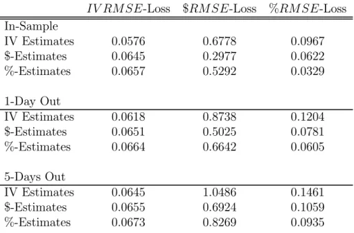
Table 3A: Average RMSE Losses for Various Estimates IV RM SE-Loss $RM SE-Loss %RM SE-Loss In-Sample IV Estimates 0.0576 0.6778 0.0967 $-Estimates 0.0645 0.2977 0.0622 %-Estimates 0.0657 0.5292 0.0329 1-Day Out IV Estimates 0.0618 0.8738 0.1204 $-Estimates 0.0651 0.5025 0.0781 %-Estimates 0.0664 0.6642 0.0605 5-Days Out IV Estimates 0.0645 1.0486 0.1461 $-Estimates 0.0655 0.6924 0.1059 %-Estimates 0.0673 0.8269 0.0935

Table 3A summarizes the information in Figures 2A and 2B by presenting the average RMSE computed over the 750 days in the sample.11 _{The diagonal on each part of the table} corresponds to the loss from using the relevant loss function in estimation. O®-diagonal entries correspondingly report the losses from using estimates which minimize a loss func-tion di®erent from the relevant one. For example, for the results in Figure 2A, we look in the middle column. We see that on average, when using the appropriate loss function to obtain the estimates µt;$, the one-day out-of-sample RMSE is 0.5025, whereas if the wrong loss function is used to obtain µt;IV, the average RMSE is 0.8738. For 5-days out-of-sample, the corresponding RMSEs are 0.6924 and 1.0486, respectively. The data in Figure 2B is summarized in the right column. Again we see large average improvements in RMSEs from using the appropriate loss function. Finally, in the left column we present evidence on an estimation exercise that was not reported in Figure 2. Whereas most studies cited above use the dollar-based loss function (1) or percentage-based loss function (2) for out-of-sample

11_{In order to compare the in-sample and one through ¯ve days out-of-sample numbers we only report}

(16)

performance evaluation, we investigate which average RMSEs one would obtain when eval-uating the square root of the IV M SE (3) out-of-sample. It can be seen that regardless of whether we evaluate the RMSEs at t, t + 1 or t + 5, we always obtain the lowest RMSEs by using the appropriate in-sample loss function. Notice however that the di®erences across es-timates in IV RMSE loss are much smaller than the di®erences across eses-timates in $RM SE and %RM SE loss.

In order to facilitate the comparison of di®erent RMSEs, Table 3B reports average RMSEs from Table 3A but normalized by the RMSE from the relevant loss function. Notice that normalized loss is always at least one. Notice also that the IV estimates fare particularly poorly when used in the other loss functions. These tables therefore illustrate our main point that it is critically important to use the correct loss function. We again stress that we are not advocating any particular loss function, but simply cautioning researchers to be consistent in their choice: The estimation loss function should ideally be the same as the evaluation loss function, or at a minimum, the estimation loss function should be identical across models. We view the existing discussion about the relative merits of certain loss functions is to some extent a moot one: The choice of loss function should be driven by user objectives. Even though some loss functions have obvious econometric problems associated with them, such as heteroskedasticity and numerical stability issues, our analysis indicates that these concerns are outweighed by the gains from matching loss functions. Regardless of the loss function of interest in model evaluation, it should also be used in estimation as long as it is reasonably well-behaved.

Table 3B: Normalized Average RMSE Losses for Various Estimates IV RM SE-Loss $RMSE-Loss %RM SE-Loss In-Sample IV Estimates 1.0000 2.2764 2.9387 $-Estimates 1.1206 1.0000 1.8898 %-Estimates 1.1409 1.7774 1.0000 1-Day Out IV Estimates 1.0000 1.7388 1.9910 $-Estimates 1.0528 1.0000 1.2908 %-Estimates 1.0744 1.3217 1.0000 5-Days Out IV Estimates 1.0000 1.5143 1.5629 $-Estimates 1.0165 1.0000 1.1328 %-Estimates 1.0440 1.1942 1.0000

(17)

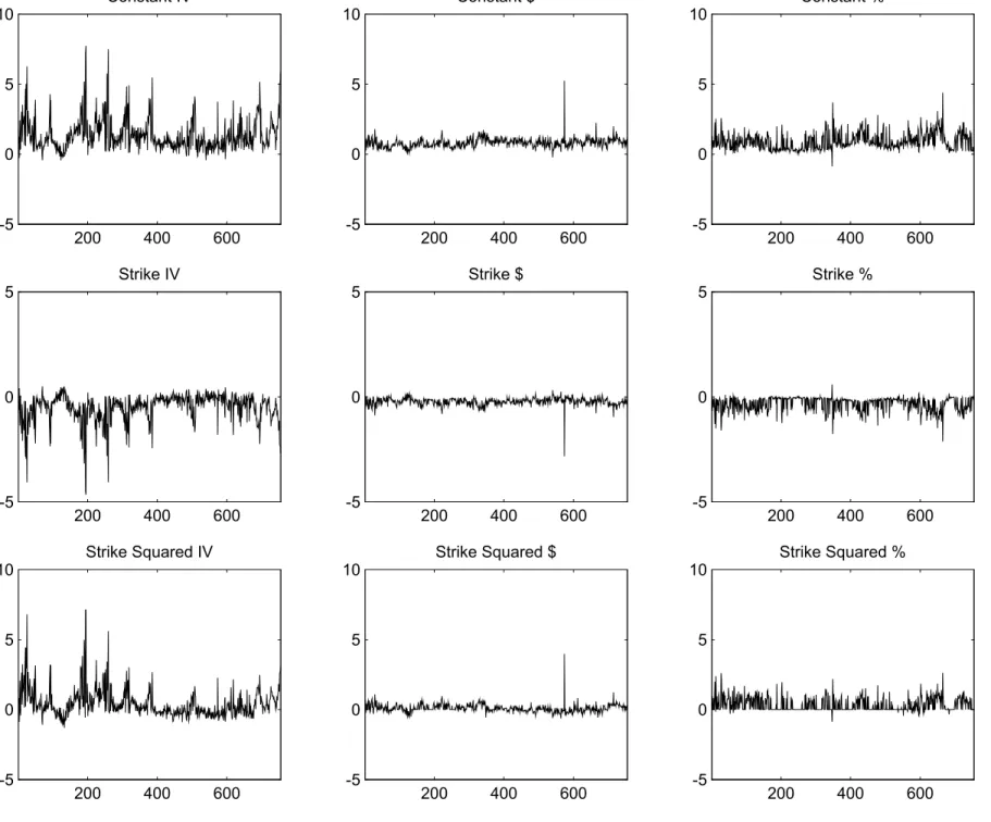
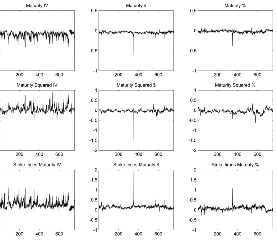
Is it possible to provide some intuition for why the IV MSE-based estimates seem so much poorer than the $-based and %-based estimates? Figures 3A and 3B graph the estimates of the coe±cients in the implied volatility relation (5) for all 755 cross-sections used, when using di®erent loss functions. The panels on the left use the IV loss function (3). The panels in the middle use the dollar based loss function (1) and the panels on the right use the percentage loss function (2). The problem with the IV M SE estimates seems to be that, although they are obtained from linear regression, they are much more volatile than the estimates from the other loss functions, which are obtained using nonlinear estimation.

Table 4 complements Figure 3 by reporting the 5th, 50th, and 95th percentile of the daily estimates for the six parameters. The parameters have been rescaled to take on reasonable values and the magnitudes are therefore not directly interpretable. This table con¯rms the variability in the IV estimates when compared with the dollar and percentage-based estimates. It appears that the dollar and percentage based estimates are more robust over time than the IV estimates, despite their nonlinear features. As a direct result their out-of-sample performance is much better.

Table 4: Parameter Estimates from Various Loss Functions: Percentiles of Daily Estimates IV M SE-Estimates Constant Strike Strike2 _{Maturity Maturity}2 _Strike_¤Maturity 5th Percentile 0.0970 -1.7932 -0.6234 -0.2496 -0.1451 0.0433 Median 1.0584 -0.3214 0.1897 -0.0824 0.0239 0.2483 95th Percentile 3.6234 0.1988 2.4775 -0.0085 0.4012 0.6828 $-Estimates 5th Percentile 0.3543 -0.4984 -0.2678 -0.0789 -0.1205 0.0447 Median 0.7983 -0.2012 0.0000 -0.0422 -0.0287 0.1427 95th Percentile 1.2843 0.0035 0.5349 -0.0106 0.0561 0.2417 %-Estimates 5th Percentile 0.2061 -0.9323 -0.0000 -0.0666 -0.2113 -0.0641 Median 0.7572 -0.1808 0.0000 -0.0173 -0.0559 0.0762 95th Percentile 2.1000 -0.0117 1.2503 0.0241 0.1092 0.2310

5 Comparison with a Structural Model

So far the empirical analysis has focused on documenting the improvement in the evaluation loss when the appropriate estimation loss is used. We now ask if the loss function issue is important enough to reverse existing empirical rankings of models. Interestingly, it is.

(18)

To document this, we compare the PBS model's pricing performance with the pricing performance of the classic stochastic volatility model proposed by Heston (1993). Heston's model assumes that the stock price under risk neutrality evolves according to

dS(t) = rSdt +qv(t)Sdz1(t) (15)

with the variance process

dv(t) = ·('_{¡ v(t))dt + ¾}qv(t)dz2(t) (16) with z1(t) and z2(t) standard Brownian motion with correlation coe±cient ½.12 The Heston model is attractive because it yields an analytical solution for the option price (up to a numerical integral that can be evaluated fast and accurately). This solution can be found in Heston (1993) and Bakshi, Cao and Chen (1997). We implement this model by estimating the four parameters ·; '; ¾ and ½. Also, because we estimate the model on a day-by-day basis, we follow the example of Bakshi, Cao and Chen (1997) and estimate the initial conditional volatility, v(0); as a ¯fth parameter each day. We estimate these parameters for $M SE as well as %M SE loss functions. We then proceed to evaluate the model in-sample and out-of-sample and to compare the pricing errors with those of the PBS model.

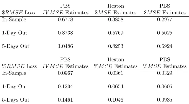
Table 5 presents average RMSE losses for the Heston model using the same 750 days of options contracts that were used to generate the empirical results in Table 3A. To facilitate comparisons between the models we repeat certain entries from Table 3A in Table 5. More detailed evidence on the day-by-day performance of the Heston model is reported in Figure 4.

Table 5 clearly illustrates that the use of the appropriate loss function is of critical impor-tance. For instance, consider the performance of the Heston model when the $RMSE loss function is used. For the in-sample evaluation the average $RMSE over 750 days is 0.3858 (middle column). Consider comparing this with the PBS model as implemented in DFW (left column). We would conclude that the Heston model beats the benchmark PBS model, because 0.3858 is lower than 0.6778. However, when the PBS model is implemented using the appropriate loss function (right column), the average $RM SE is 0.2977. Therefore, the structural model actually does not perform better than the modi¯ed PBS model.13 _Similarly, inspecting the $RMSE loss functions evaluated out-of-sample, we see that the average 1-day and 5-1-day out-of-sample $RM SEs are 0.5769 and 0.8253, higher than 0.5025 and 0.6924

12_{It is well-known from a number of recent papers that the empirical performance of this model is not}

entirely satisfactory and that extending the model can improve its pricing performance (see Andersen, Benzoni and Lund (1999), Bakshi, Cao and Chen (1997), Benzoni (1998), Chernov and Ghysels (2000), Jones (2001) and Pan (2000)). We simply want to compare di®erent implementations of the PBS model to a mainstream structural model that is easy to implement and which ¯ts the data reasonably well.

13_{Notice that while the Heston model nests the original Black and Scholes (1973) model it does not nest}

(19)

respectively for the PBS model. If we had used the standard IV MSE-implementation of the model we would have concluded that 0.5769 and 0.8253 are lower than 0.8738 and 1.0486 respectively.

Table 5: Average RMSE Losses for Heston and PBS Models

PBS Heston PBS

$RM SE Loss IV M SE Estimates $M SE Estimates $MSE Estimates

In-Sample 0.6778 0.3858 0.2977

1-Day Out 0.8738 0.5769 0.5025

5-Days Out 1.0486 0.8253 0.6924

PBS Heston PBS

%RMSE Loss IV M SE Estimates %M SE Estimates %M SE Estimates

In-Sample 0.0967 0.0361 0.0329

1-Day Out 0.1204 0.0654 0.0605

5-Days Out 0.1461 0.1046 0.0935

Inspection of the second set of rows in Table 5 shows that identical conclusions obtain when evaluating %RM SE loss functions. For the in-sample evaluation, the average Heston %RM SE of 0.0361 is lower than 0.0967 but higher than 0.0329. For the 1-day out-of-sample exercise the average Heston %RM SE of 0.0654 is lower than 0.1204 but higher than 0.0605. Finally, for the 5-day out-of-sample exercise the average Heston %RM SE of 0.1046 is lower than 0.1461 but higher than 0.0935. In summary, the conclusions from the comparison of the Heston model with the PBS model are robust. Regardless of whether one uses $RM SE or %RM SE loss functions, and regardless of whether one evaluates the loss functions in-sample or out-of-sample, the PBS model performs better than the Heston model when implemented using the appropriate loss function. However, when the PBS model is implemented using the IV M SE loss function to estimate the parameters, which is the standard in the literature, it cannot improve upon the performance of the Heston model.

6 Conclusions

This paper raises an important methodological issue concerning the estimation of parameters for use in option pricing models. Until now, the literature has mainly focused on the choice of option pricing model. Once the model is chosen, the main concern is the consistent and

(20)

e±cient econometric estimation of the parameters characterizing the model. The focus is thus much more on estimation as opposed to evaluation of the model. We argue that the relevant discussion should not start out by discussing how to estimate the parameters, but rather by stating what the evaluation (typically out-of-sample) loss function is. This loss function is dictated by the purpose of the empirical exercise and can be related to a hedging problem or a risky investment strategy for example.

It may be di±cult at ¯rst to intuitively grasp why this issue is of more than philosophical importance. The key is that one should stop thinking about the search for a \true" model. Instead, we are searching for parsimonious models that are inherently misspeci¯ed and that ¯t certain features of the data better than others. If the model under investigation is the \true" model, it does not matter which loss function we use. We always obtain the same \true" parameters. This is the mind-set inspiring much of current practice, which puts a lot of emphasis on e±cient econometric estimation. We argue that the focus should be on the minimization of the loss function used in evaluation. The standard econometric solution to this problem when working with misspeci¯ed models is to use an in-sample estimation loss function identical to the out-of-sample evaluation loss function.

The paper then demonstrates that this approach is of great practical importance. To do this, we focus on the simplest model available in the literature that attempts to account for the well-known biases in the Black-Scholes model, namely the Practitioner Black-Scholes (PBS) model. The PBS model is typically implemented with an estimation loss function which is di®erent from the evaluation loss function, and this constitutes a problem. Our analysis shows that this problem is quantitatively important, with the implementation used in the literature leading to out-of-sample RMSEs that are more than twice the lowest possible RMSE using the proper estimation loss function. This ¯nding has serious implications for future studies and for papers that have implemented this technique the traditional way. To demonstrate these implications, we compare the empirical performance of the PBS model to the performance of a well-known stochastic volatility model due to Heston (1993). We ¯nd that when the PBS model is implemented using an inappropriate loss function, it performs much worse than the Heston model. However, the PBS model performs somewhat better than the Heston model when the appropriate loss function is used. Thus our modi¯ed PBS model represents a new and tougher standard against which the performance of future structural models can be measured.

(21)

References

[1] Ait-Sahalia, Y. and A. Lo (1998), \Nonparametric Estimation of State-Price Densities Implicit in Financial Asset Prices," Journal of Finance, 53, 499-547.

[2] Andersen, T., Benzoni, L. and J. Lund (1999), \Estimating Jump-Di®usions for Equity returns," Manuscript, Northwestern University.

[3] Bakshi, C., Cao, C. and Z. Chen (1997), \Empirical Performance of Alternative Option Pricing Models," Journal of Finance, 52, 2003-2049.

[4] Bates, D. (1996a), \Jumps and Stochastic Volatility: Exchange Rate Processes Implicit in Deutsche Mark Options," Review of Financial Studies, 9, 69-107.

[5] Bates, D. (1996b), \Testing Option Pricing Models," in G.S. Maddala and C.R. Rao, eds.: Handbook of Statistics, Vol 15: Statistical Methods in Finance (North-Holland, Amsterdam), 567-611.

[6] Benzoni, L. (1998), \Pricing Options Under Stochastic Volatility: An Econometric Anal-ysis," Manuscript, University of Minnesota.

[7] Black, F. and M. Scholes (1973), \The Pricing of Options and Corporate Liabilities," Journal of Political Economy, 81, 637-659.

[8] Campbell, J., Lo, A. and C. MacKinlay (1997), \The Econometrics of Financial Mar-kets," Princeton University Press.

[9] Chernov, M. and E. Ghysels, (2000) \A Study Towards a Uni¯ed Approach to the Joint Estimation of Objective and Risk Neutral Measures for the Purpose of Option Valuation," Journal of Financial Economics, 56, 407-458.

[10] Derman, E., and I. Kani (1994), \Riding on the Smile," Risk, 7, 32-39.

[11] Duan, J. (1995), \The GARCH Option Pricing Model," Mathematical Finance, 5, 13-32. [12] Dumas, B., Fleming, F. and R. Whaley (1998), \Implied Volatility Functions: Empirical

Tests," Journal of Finance, 53, 2059-2106.

[13] Dupire, B. (1994), \Pricing with a Smile," Risk, 7, 18-20.

[14] Garcia, R., R. Luger and E. Renault (2000), \Empirical Assessment of an Intertem-poral Option Pricing Model with Latent Variables," Manuscript, CRDE, Universite de Montreal.

(22)

[15] Hausman, J. (1978), \Misspeci¯cation Tests in Econometrics," Econometrica, 46, 1251-1271.

[16] Heston, S. (1993), \A Closed-Form Solution for Options with Stochastic Volatility with Applications to Bond and Currency Options," Review of Financial Studies, 6, 327-343. [17] Heston, S. and S. Nandi (2000), \A Closed-Form GARCH Option Pricing Model,"

Review of Financial Studies, 13, 585-626.

[18] Hull, J. and A. White (1987), \The Pricing of Options with Stochastic Volatilities," Journal of Finance, 42, 281-300.

[19] Hull, J. and W. Suo (2000), \A Methodology for Assessing Model risk and its Ap-plication to the Implied Volatility Function Model," Manuscript, Rotman School of Management, University of Toronto.

[20] Hutchinson, J., Lo, A. and T. Poggio (1994), \A Nonparametric Approach to Pricing and Hedging Derivative Securities Via Learning Networks," Journal of Finance, 49, 851-889.

[21] Jacquier, E. and R. Jarrow (2000), \Bayesian Analysis of Contingent Claim Model Error," Journal of Econometrics, 94, 145-180.

[22] Jones, C. (2000), \The Dynamics of Stochastic Volatility," Manuscript, University of Rochester.

[23] Jones, C. (2001), \A Nonlinear Analysis of S&P 500 Index Option Returns," Manuscript, Simon School of Business, University of Rochester.

[24] Melino, A. and S. Turnbull (1990), \Pricing Foreign Currency Options with Stochastic Volatility," Journal of Econometrics, 45, 239-265.

[25] Nandi, S. (1998), \How Important is the Correlation Between returns and Volatility in a Stochastic Volatility Model? Empirical Evidence from Pricing and Hedging in the S&P 500 Index Options Market," Journal of Banking and Finance 22, 589-610.

[26] Pan, J. (2000), \Integrated Time-Series Analysis of Spot and Option Pricing," Manuscript, MIT Sloan School of Management.

[27] Renault, E. (1997), \Econometric Models of Option Pricing Errors," Advances in Eco-nomics and Econometrics: Theory and Applications: Seventh World Congress. Volume 3. (Kreps, D. and K. Wallis, eds.), Econometric Society Monographs, no. 28. Cambridge; New York and Melbourne: Cambridge University Press, 223-78.

(23)

[28] Rosenberg, J. and R. Engle, (2000), \Empirical Pricing Kernels," Manuscript, NYU-Stern School of Business.

[29] Rubinstein, M. (1994), \Implied Binomial Trees," Journal of Finance, 49, 771-818. [30] Scott, L. (1987), \Option Pricing when the Variance Changes Randomly: Theory,

Esti-mators and Applications," Journal of Financial and Quantitative Analysis, 22, 419-438. [31] White, H. (1981), \Consequences and Detection of Misspeci¯ed Nonlinear Regression

(24)

0.16 0.18 0.2 0.22 0.24 0.26 0.28 0.3

(25)

100 200 300 400 500 600 700 0

2 4 6

8 In-Sample $-RMSE, IV-Estimates

100 200 300 400 500 600 700

0 2 4 6

8 In-Sample $-RMSE, $-Estimates

100 200 300 400 500 600 700

0 2 4 6

8 1-Day Out $-RMSE, IV-Estimates

100 200 300 400 500 600 700

0 2 4 6

8 1-Day Out $-RMSE, $-Estimates

2 4 6

8 5-Days Out $-RMSE, IV-Estimates

2 4 6

8 5-Days Out $-RMSE, $-Estimates

(26)

100 200 300 400 500 600 700 0 0.2 0.4 0.6 0.8

1 In-Sample %-RMSE, IV-Estimates

100 200 300 400 500 600 700 0 0.2 0.4 0.6 0.8

1 In-Sample %-RMSE, %-Estimates

100 200 300 400 500 600 700 0 0.2 0.4 0.6 0.8

1 1-Day Out %-RMSE, IV-Estimates

100 200 300 400 500 600 700 0 0.2 0.4 0.6 0.8

1 1-Day Out %-RMSE, %-Estimates

0.2 0.4 0.6 0.8

1 5-Days Out %-RMSE, IV-Estimates

0.2 0.4 0.6 0.8

1 5-Days Out %-RMSE, %-Estimates

(27)

200 400 600 -5 0 5 10 Constant IV 200 400 600 -5 0 5 Strike IV 0 5 10 Strike Squared IV 200 400 600 -5 0 5 10 Constant $ 200 400 600 -5 0 5 Strike $ 0 5 10 Strike Squared $ 200 400 600 -5 0 5 10 Constant % 200 400 600 -5 0 5 Strike % 0 5 10 Strike Squared %

(28)

200 400 600 -1 -0.5 0 0.5 Maturity IV 200 400 600 -2 -1.5 -1 -0.5 0 0.5 1 Maturity Squared IV -0.5 0 0.5 1 1.5

2 Strike times Maturity IV

200 400 600 -1 -0.5 0 0.5 Maturity $ 200 400 600 -2 -1.5 -1 -0.5 0 0.5 1 Maturity Squared $ -0.5 0 0.5 1 1.5

2 Strike times Maturity $

200 400 600 -1 -0.5 0 0.5 Maturity % 200 400 600 -2 -1.5 -1 -0.5 0 0.5 1 Maturity Squared % -0.5 0 0.5 1 1.5

2 Strike times Maturity %

(29)

0 100 200 300 400 500 600 700 0 0.2 0.4 0.6 0.8

1 In-Sample %-RMSE for Heston model

0 100 200 300 400 500 600 700

0 2 4 6

8 In-Sample $-RMSE for Heston model

0 100 200 300 400 500 600 700 0 0.2 0.4 0.6 0.8

1 1-Day Out-of-Sample %-RMSE for Heston model

0 100 200 300 400 500 600 700

0 2 4 6

8 1-Day Out-of-Sample $-RMSE for Heston model

0.2 0.4 0.6 0.8

1 5-Day Out-of-Sample %-RMSE for Heston model

2 4 6

8 5-Day Out-of-Sample $-RMSE for Heston model

(30)

Liste des publications au CIRANO*

Série Scientifique / Scientific Series (ISSN 1198-8177)

2001s-44 Let’s Get "Real" about Using Economic Data / Peter Christoffersen, Eric Ghysels et Norman R. Swanson

2001s-43 Fragmentation, Outsourcing and the Service Sector / Ngo Van Long, Ray Riezman et Antoine Soubeyran

2001s-42 Nonlinear Features of Realized FX Volatility / John M. Maheu et Thomas H. McCurdy

2001s-41 Job Satisfaction and Quits: Theory and Evidence from the German

Socioeconomic Panel / Louis Lévy-Garboua, Claude Montmarquette et Véronique Simonnet

2001s-40 Logique et tests d'hypothèse : réflexions sur les problèmes mal posés en économétrie / Jean-Marie Dufour

2001s-39 Managing IT Outsourcing Risk: Lessons Learned / Benoit A. Aubert, Suzanne Rivard et Michel Patry

2001s-38 Organizational Design of R&D Activities / Stefan Ambec et Michel Poitevin 2001s-37 Environmental Policy, Public Interest and Political Market / Georges A. Tanguay,

Paul Lanoie et Jérôme Moreau

2001s-36 Wealth Distribution, Entrepreneurship and Intertemporal Trade / Sanjay Banerji et Ngo Van Long

2001s-35 Comparaison des politiques de rémunération en fonction des stratégies organisationnelles / Michel Tremblay et Denis Chênevert

2001s-34 Déterminants et efficacité des stratégies de rémunération : Une étude internationale des entreprises à forte intensité technologique / Michel Tremblay, Denis Chênevert et Bruno Sire

2001s-33 La multiplicité des ancres de carrière chez les ingénieurs québécois: impacts sur les cheminements et le succès de carrière / Yvon Martineau, Thierry Wils et Michel Tremblay

2001s-32 The Impact of Interface Quality on Trust in Web Retailers / Marie-Christine Roy, Olivier Dewit et Benoit A. Aubert

2001s-31 R&D and Patents: Which Way Does the Causality Run? / Hans van Ophem, Erik Brouwer, Alfred Kleinknecht and Pierre Mohnen

2001s-30 Contracting under Ex Post Moral Hazard and Non-Commitment / M. Martin Boyer

2001s-29 Project Financing when the Principal Cannot Commit / M. Martin Boyer

2001s-28 Complementarities in Innovation Policy / Pierre Mohnen et Lars-Hendrick Röller 2001s-27 Bankruptcy Cost, Financial Structure and Technological Flexibility Choices /

Marcel Boyer, Armel Jacques et Michel Moreaux