Revisiting Subnet Inference WISE-ly
Jean-François Grailet, Benoit Donnet
Université de Liège, Montefiore Institute, Belgium
Abstract—Since the late 90’s, the Internet topology discovery has been an attractive and important research topic, leading, among others, to multiple probing and data analysis tools developed by the research community. This paper looks at the particular problem of discovering subnets (i.e., a set of devices that are located on the same connection medium and that can communicate directly with each other at the link layer).
In this paper, we first show that the use of traffic engineering policies may increase the difficulty of subnet inference. We care-fully characterize those difficulties and quantify their prevalence in the wild. Next, we introduce WISE (Wide and lInear Subnet inferencE), a novel tool for subnet inference designed to deal with those issues and able to discover subnets on wide ranges of IP addresses in a linear time. Using two groundtruth networks, we demonstrate that WISE performs better than state-of-the-art tools while being competitive in terms of subnet accuracy. We also show, through large-scale measurements, that the selection of vantage point with WISE does not matter in terms of subnet accuracy. Finally, all our code (WISE, data processing, results plotting) and collected data are freely available.
I. INTRODUCTION
For now nearly two decades, the Internet topology has been investigated at multiple levels [1]. The most basic point of view is the IP interface level where data is revealed through hop-by-hop exploration performed by traceroute and variants (see, e.g., Paris traceroute [2]). Second, multiple interfaces of a given router might be aggregated into a single identifier thanks to alias resolution. Finally, the higher level would be the Autonomous System (AS) level which models relationships between ASes and is captured, for instance, through BGP routing information.
Besides this academic view of the Internet topology, new intermediate levels have emerged over time. For instance, Internet eXchange Points (IXPs) [3], [4] or Points-of-Presence (PoPs) [5], [6] are more and more investigated. This paper is in the scope of an another intermediate level: sub-networks (or, more simply, subnets), i.e., a set of devices that are located on the same connection medium and that can communicate directly with each other at the link layer [7]. Exploring subnets is a way to enrich router level maps by providing particular topological features of ISP networks.
Standard techniques for revealing subnets are based on active probing and on-the-fly complex rules for building each subnet [8], [9], [10]. However, those tools fail to reveal accurate subnets in the presence of traffic engineering policies, such as load balancing [11], applied by domains.
In this paper, we first review the most common phenomena which increase the difficulty of subnet inference for classical tools and elaborate on what kind of traffic engineering policies could cause them. Second, we introduce a novel tool, WISE
(Wide and lInear Subnet inferencE), which is designed to detect these phenomena and take them into account upon discovering subnets. WISE not only carefully evaluates the IP addresses considered for subnet inference, but it also achieves it without additional probing and in linear time (i.e., the execution time will be proportional to the amount of addresses considered for subnet inference). Indeed, WISE is built to first collect the data it needs for subnet inference , while previous state-of-the-art tools [8], [9], [10] usually discovers subnets while probing.
Our contributions include a first characterization and evalua-tion of modern subnet inference challenges, a new tool (WISE) that can work around these issues while performing overall better than state-of-the-art tools and an evaluation of the effects of changing the vantage point from one measurement to another, as encountered traffic engineering issues will likely change as well. With this, we demonstrate that WISE can usually withstand vantage point change pretty well despite some punctual drastic updates in the collected data. The source code of WISE, our figures, and the scripts for generating them (or scheduling a campaign) are all available online.1
The remainder of this paper is organized as follows: Sec. II discusses and quantifies challenges faced by traditional subnet inference tools; Sec. III introduces WISE, our novel subnet inference tool; Sec. IV validates WISE with respect to state-of-the-art tools based on two groundtruths; Sec. V evaluates WISEperformance in the wild; finally, Sec. VI concludes this paper by summarizing its main achievements.
II. SUBNETINFERENCECHALLENGES
In this section, we discuss the different challenges that can arise when one attempts to infer the subnets contained in a target domain.
A. State-of-the-Art inference
A subnetwork, or subnet, consists in a set of devices, each of them being identified by a unique IP address, that all are connected together through the same connection medium. In the Internet, a subnet can be a point-to-point link as well as a local area network (LAN) isolated in the network topology. From a measurement perspective, in the (near) absence of any traffic engineering, subnet interfaces will appear as a set of interfaces that are consecutive with respect to the IP scope, that are located at the same distance in Time-To-Live (or TTL), i.e., the minimal TTL value to use to get a reply from the subnet, and that are reached through the same route in the network
topology, i.e., the last interface appearing in the route towards each subnet interface is the same for each route.
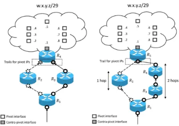
Ideally, a subnet should also contain at least one interface that belongs to the last router crossed before entering the subnet, and which therefore appears one hop closer to the measurement vantage point than other subnet interfaces. In TraceNET [8] and ExploreNET [9] terminology (as well as TreeNET [10]), interfaces belonging to the subnet that are not located on the last crossed router are called pivot interfaces while the interface(s) located on this router are called contra-pivot interfaces, as illustrated in Fig. 1 (pivots are white squares, while contra-pivots are depicted by gray squares). It should be noted that, while having a single contra-pivot interface makes more sense at first glance, it is actually possible to find more than one contra-pivot because routers may implement back-up interfaces to reach critical subnets. In practice, we have observed such a scenario in the groundtruth we used for our validation (see Sec. IV).
All state-of-the-art tools take advantage of those ideas to reveal subnets. TraceNET uses traceroute-like probing towards a set of target IP addresses and, then, analyzes the collected routes to identify the subnets crossed to reach the destinations. ExploreNET probes a growing range of IP addresses consecutively (starting with a single initial target, then building a /31 or /30, then a /29, etc.) to build a subnet that keeps expanding as long as a few rules are fulfilled and as long as responsive interfaces can be found. Finally, TreeNET builds itself upon ExploreNET and provides algorithmic corrections to better identify larger subnets, specially when the probed subnet lacks of responsive interfaces.
It should be noted that subnet inference has also been explored with passive techniques, with tools that require to send multiple probes in the network but with additional post-processing (without probing) to infer the subnets. For instance, IGMP probing [12] allows to reveal subnets by applying several rules (e.g., routers must be connected through the same Layer-2 device) to the collected data. However, nowadays, IGMP probing is not anymore useful as it is heavily filtered by operators [13].
B. Subnet Inference Obstacles
Unfortunately, no matter the tool, state-of-the-art subnet inference relies on strong hypotheses. For instance, all tools assume that interfaces from a given subnet will necessarily appear at the same distance in term of minimal TTL, and that the last hop before these interfaces will also be the same. We identify no less than three phenomena that have the potential to violate those assumptions: flickering IP addresses, warping IP addresses, and echoing IP addresses.
Before describing those phenomena, we introduce the notion of trail. A trail denotes the last interface seen in the route (obtained by performing traceroute-like probing) before a given target IP address. However, the last interface in the route towards a given target address is not always visible. Therefore, we generalize the notion of trail such that it corresponds to the last non-anonymous and not cycling interface in the route
(a) Flickering IP addresses. (b) Warping IP addresses.
Fig. 1. Issues with the last interface(s) before the subnet (plain bullets). Plain and dashed paths are different routes.
towards the target IP address. In addition, we also associate to the trail the amount of subsequent hops that are either anonymous hops or cycling hops, called anomalies.
Flickering and warping are potential artifacts of IP load-balancing occurring just before the IP interfaces that appear in trails. IP load-balancing [11] leads to a subgraph that is delimited by a divergence point (the router performing the load-balancing, e.g., R1 in Fig. 1) followed, two or more
hops later, by a convergence point (e.g., R4 in Fig. 1a and
R5 in Fig. 1b). This subgraph forms a diamond with multiple
branches between the divergence and convergence point. Au-gustin et al. [11] considered a diamond being symmetric if all parallel paths feature the same number of hops, otherwise it is said to be asymmetric.
On one hand, flickering, as illustrated in Fig. 1a, refers to a situation in which we observe multiple IP addresses acting as the trail for pivot interfaces of a given subnet, all of them being located at the same distance (in terms of TTL) from the vantage point. We say these addresses are flickering because they usually appear in turns if we consider a bunch of subnet interfaces that are close and consecutive regarding the address space. We believe that flickering is mainly caused by symmet-ric load-balanced paths. Performing alias resolution between flickering addresses can confirm this assumption: in several of our measurements of the autonomous system AS6453 (Tata Communications), we were able to alias together more than half of the detected flickering addresses. It was achieved by using an alias resolution framework originally implemented in TreeNET[14]. It consists (to put it simply) in fingerprinting IP addresses [15] that could be aliases of each other to select the most suited state-of-the-art alias resolution method. In the case of AS6453, most addresses were aliased with Ally [16] and iffinder [17], both methods being usually very reliable on small sets of IP addresses. For instance, on February 19th, 2019, 37 addresses out of the 62 detected flickering interfaces could be aliased together, and there were as much as 84 aliased addresses on a total of 119 on the next day (the measurement
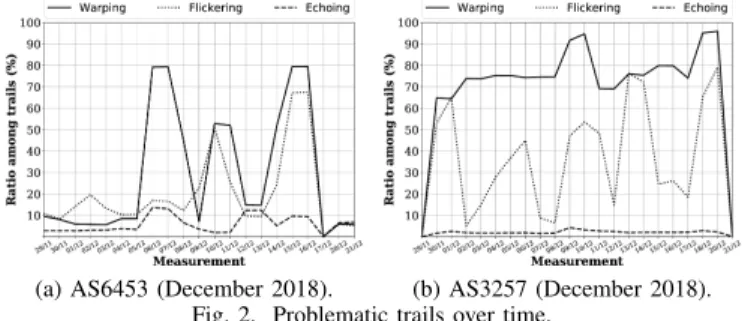
(a) AS6453 (December 2018). (b) AS3257 (December 2018). Fig. 2. Problematic trails over time.
being done from a different vantage point). 2
On the other hand, warping (illustrated in Fig. 1b) is likely caused by asymmetric load-balancing. We indeed see the same IP address acting as the trail for the pivot interfaces of a given subnet while being observed at different distances (in terms of TTL), depending on the pivot. In such a scenario, pivot interfaces and their respective trails are thus reached through different routes whose lengths vary from one probe to another. Finally, echoing refers to a very specific issue that is the consequence of the configuration of some specific brands of routers. Upon the reception of a packet targeting a close-by interface (i.e., one hop away) whose the TTL value has expired, these routers will reply with a time-exceeded message in which the source IP address will be the target itself rather than an interface of the replying router. As a consequence, the IP address acting as the trail is not an interface of the ingress router (i.e., the last router crossed before the subnet) but the target address itself. We therefore say the trail is echoing the target.
C. Inference Obstacles in the Wild
During Fall 2018, we measured 22 different ASes (i.e., Autonomous Systems) from 22 different vantage points in the PlanetLab testbed in order to quantify flickering, warping, and echoing. Measurements were performed on a daily basis and each target AS was probed by a different vantage point over the various runs. Doing so, we were able to investigate how the choice of a Vantage Point may impact flickering, warping, and echoing.
For each target AS, we plot a figure in which we show, for each collected dataset (X-Axis – dataset date in DD/MM format), the ratio of trails (Y-Axis) suffering from flickering (dotted line), warping (plain line), and echoing (dashed line). We computed a ratio as the number of trails suffering from a given issue to the total number of discovered trails (the same trail may thus appear multiple times). We do so to avoid under-evaluating warping and flickering. Indeed, as echoing trails are almost always unique, they would appear as over-represented with a ratio based on unique trails, while, in practice, they appear for much less target IP addresses than both warping and flickering.
Due to space constraints, we will focus, in this paper, on typical cases. We therefore encourage readers to check
2Cfr. https://github.com/JefGrailet/WISE/tree/master/Dataset/AS6453/
2019/02
our public repository 3 to get access to all figures (but also
our scripts and datasets). Fig. 2a shows the extent of all three issues for AS6453, using datasets collected from late November 2018 to shortly before Christmas 2018. With the exception of one dataset collected from a vantage point that had poor reachability (December 17th), all issues appear in
almost every dataset. Three spikes (corresponding in practice to six datasets) are visible and are due to warping trails ratio drastically increasing. Interestingly, the flickering ratio also spikes but only for three of these six datasets, and stays below 20% (a fairly common observation with this particular AS) for the first "hill" observed for warping trails. This supports the idea that both issues are caused by different kinds of traffic engineering (most probably load-balancing), as we discussed in Sec. II-B.
For the sake of comparison, we also provide results for AS3257 (GTT Communications) in Fig. 2b. Here, a large majority of trails correspond to warping trails, no matter the vantage point (first and last dataset corresponding to PlanetLab nodes located at that same geographical location with poor reachability). However, the ratio of trails which corresponds to flickering trails vary a lot from one dataset to another, further supporting our hypothesis that both warping and flickering are the results of different traffic engineering strategies. We finally note that there is a low, yet noticeable amount of echoing trails in all datasets. The weak variations might be simply explained by the fact that the total of responsive interfaces vary from one dataset to another. Likewise, in the case of AS6453, the small spikes in echoing trails match datasets that contained more responsive interfaces. In other words, the presence of echoing trails is likely not a consequence of traffic engineering, but rather a matter of what kind of device is used in the surroundings of target addresses.
III. WISE
In order to address carefully the issues described up to this point, we introduce a new tool called Wide and lInear Subnet inferencE (WISE). Not only WISE is designed to provide a renewed subnet inference taking account of the issues previously discussed, but it is also designed to discover subnets on wide ranges of IP addresses in a linear time. Indeed, despite using multi-threading and sometimes implementing heuristics to speed up subnet inference, state-of-the-art tools such as TreeNET [10] can still require either several days of measurements, or several vantage points in order to fully measure a target domain whose prefixes cover several millions of IP addresses. Such an amount of resources can be a problem to schedule large measurement campaigns. This is why WISE also puts the emphasis on achieving linear complexity for all its major algorithmic steps (Sec. III-D).
Indeed, given a set of target IPv4 prefixes4belonging to the
target domain5, WISE works as a succession of three stages:
target pre-scanning (Sec. III-A), target scanning (Sec. III-B),
3https://github.com/JefGrailet/WISE/tree/master/Evaluation/Obstacles
4WISEis currently only implemented for IPv4.
and finally the subnet inference itself (Sec. III-C). It is worth noting that the two first stages are the only algorithmic steps requiring active probing. Due to space constraints, we will not cover all the algorithms implemented by WISE in details in this paper and we will stick to the main and most important ideas. Interested readers can, of course, review the source code to learn more about the matter.6
A. Target Pre-Scanning
The first step towards subnet inference, the aggregation of IP interfaces under a single identifier on the basis of their network location, is to check which IP addresses are alive and reachable. This is the objective pursued by “target pre-scanning”: it works by sending a single probe (typically an ICMP one but UDP and TCP can also be considered) with a large enough TTL value towards every possible IP address encompassed by the initial target prefixes and awaits for a reply. If no reply is received within a given delay, the target address will not be probed in subsequent steps.
In practice, WISE conducts pre-scanning by listing all target addresses and sharing the probing load between multiple threads in order to speed up the whole process. WISE also does a second pre-scanning only with unresponsive addresses (during the first measurement round). This second run is still scheduled with multiple threads but with the initial timeout value doubled. This ensures unresponsive addresses are indeed dead and not unreachable because of some particular network conditions. Notice that WISE may allow a third pre-scanning run at user’s will. However, two rounds should be enough.7
B. Target Scanning
Once all responsive addresses have been collected by WISE, the next step consists in collecting the data required for subnet inference (the so-called “target scanning”). We are only interested by two pieces of information: an estimation of the target distance as a minimal TTL value and its trail, as defined in Sec. II-B. To obtain this information, for every IP address in the target domain, WISE performs hop-limited probing (i.e., traceroute) and stops when it has received its first reply from the targeted IP address. Then, WISE performs some backward probing (i.e., from the target back to the vantage point) to ensure no reply could be obtained closer to the vantage point. Interfaces revealed along the path are used to both estimate the distance in TTL and find the trail.
In practice, WISE does not perform a complete
traceroute towards each target IP address. Indeed, IP addresses are ranged in increasing order, based on their numerical equivalent. Consequently, when WISE knows the TTL distance required to reach a given IP address, it uses this TTL in the first probe towards the next IP address in the list, then adjust with possible additional forward/backward probing depending on the first probe outcome.
6https://github.com/JefGrailet/WISE/tree/master/v1/
7It should be noted that pre-scanning is not novel, as it was already
implemented and used with success with TreeNET [10].
The overall process is further sped up with multi-threading, and completed with a second measurement round to minimize the amount of situations where the last hops towards a given target address are anonymous hops or cycles.
At the end of the target scanning, WISE processes the data it collected in order to detect all flickering, warping, or echoing trails. In particular, it will make a census of all flickering trails and group these addresses depending on other addresses they are flickering with. On that basis, it will conduct alias resolution on each group to ensure we are in the scenario described in Sec. II-B or if the flickering is caused by something else (in which case WISE will not make any risky hypothesis during the subnet inference). The alias resolution currently implemented in WISE re-uses a methodology introduced by TreeNET, mainly using network fingerprinting [15] as a way to select the most suitable state-of-the-art alias resolution technique for a selection of aliasable interfaces [14].
C. Subnet inference with WISE
The subnet inference essentially consists in processing the scanned IP addresses after sorting them with respect to the IP scope (i.e., sorted according to their value as a 32-bit integer) to discover the subnets that best accommodate subsets of consecutive addresses. More precisely, WISE typically starts by removing an address from the sorted list, builds a /32 subnet for it, then progressively decreases its prefix length and retrieves from the initial list all interfaces that are encom-passed by the expanded subnet. It then proceeds to check if encompassed addresses are indeed on the same subnet, also checking if some contra-pivot(s) is (are) among them. Next, it evaluates the situation as a whole to decide whether the prefix length should be decreased furthermore or if the expansion of the subnet should be stopped, with or without increasing once its prefix length (i.e., subnet shrinkage). This will notably occur if newly encompassed addresses are incompatible with the subnet being inferred.
To check if an address belongs to the subnet, WISE selects the first pivot IP interface in the initial subnet (denoted as a reference pivot) then compares the newly encompassed interfaces (named candidate interfaces) with it. To decide whether a candidate interface and the reference pivot are on the same subnet, WISE checks up to five inference rules, all corresponding to different scenarii. If both addresses verify at least one rule, then they will be considered as being part of the same subnet.
The five inference rules are the following:
• Rule 1: both addresses have the same trail.
• Rule 2: both addresses do not share the same trail, but are located at the same TTL distance and their trails differ regarding anomalies (as explained in Sec. II-B).
• Rule 3: both addresses are located at the same TTL distance and exhibit echoing trails.
• Rule 4: both addresses are located at the same TTL
distance and their trails, previously aliased, are flickering with each other.
• Rule 5: both addresses are not located at the same TTL
distance and do not share the same trail. However, trail addresses were aliased during the analysis of flickering IP interfaces, meaning they belong to the same device reached through asymmetrical paths.
It should be noted that rule 2 is a way to ensure that an IP interface located at the same distance as all other IP addresses in a subnet is not identified as an outlier because its trail could not be discovered accurately (most likely because of a network issue). While testing this rule, WISE also considers replacing the reference pivot if the candidate address has a better trail (i.e., less or no anomalies). Addresses not satisfying any rule will be considered as potential contra-pivots if their TTL distance is lower than for pivots, and outliers otherwise. When all candidate addresses have been checked, WISE checks how many of them were identified on the subnet and how many potential contra-pivots were found to consider stopping the subnet growth or going further. Typically, WISE keeps expanding when no outlier has been found or when outliers are a minority among candidate IP addresses.8 It will
shrink otherwise, and also stop if it discovers valid contra-pivots (because the subnet will be already sound at this point). It will also shrink if there are too many possible contra-pivots (because they could actually be pivots of another subnet). Of course, WISE also has to consider some specific scenarii (like when the selected pivot turns out to be a contra-pivot), but we will leave these details for interested readers.9
We however note two things. First, WISE processes back-wards the addresses list. Indeed, many of our observations showed that contra-pivots are usually found among the first subnet addresses. Going backwards therefore ensures we can maximize the final subnet size, as going the other way around might prematurely stop the inference. Second, WISE also im-plements a subnet post-processing stage to merge consecutive (with respect to the address space) subnets whose pivots look to be on the same subnet, if they were flagged as potentially undergrown during inference (e.g., if expanding them made them overlap previously inferred subnet containing a contra-pivot) to fix situations where a subnet might be split in several chunks. It should be noted, however, that the current post-processing is still being improved. We believe, however, that careful inference as performed by WISE combined with careful post-processing could lead to overall better inference. D. Complexity
We argue that the subnet inference has a linear complexity with respects to the amount of addresses to aggregate in subnets. There are two possible worst cases which could lead to a given interface being considered multiple times. The first scenario is the one where the network exclusively consists of very small subnets containing a single interface (e.g., a /32 or /31 prefix). Upon expanding the subnet to consider
8Currently, WISE considers outliers a minority if there make up less than
1/3 of candidate addresses. This will become a parameter in a future release.
9https://github.com/JefGrailet/WISE/tree/master/v1/
a smaller prefix length, one or two other IP addresses will be encompassed, but as they will not be compatible with the current interface, it will be put back in the list of interfaces and therefore considered a second time at the next iteration. Therefore, in this scenario, all addresses are considered up to three times, which remains a bounded amount of times. The other worst possible scenario is the one where the network consists of consecutive subnets which the prefix length slowly increases. Indeed, the last expansion (assuming it occurs) of the first will encompass all other IPs, but as they are on dif-ferent subnets, they will be put back in the list, after what the same scenario will occur but on a smaller scale. In the end, the interfaces of the smallest subnet will be considered as many times as they are subnets. However, if we compute the amount of times an interface (no matter the subnet) is evaluated, then it is bounded by N + N/2 + N/4 + ... = 2N (where N is the amount of interfaces). Therefore, the complexity of subnet inference as done by WISE is linear.
IV. VALIDATION
In this section, we validate, relying on groundtruth topolo-gies, the ability of WISE to accurately reveal subnets and to perform overall better than state-of-the-art tools.
A. Methodology
To validate WISE, we measure two groundtruth topolo-gies with both WISE and a state-of-the-art tool: TreeNET. TreeNET [10] is a topology discovery tool built upon ExploreNET[9] by adding subnet refinement algorithms and heuristics, leading to a better subnet inference and a lower execution time. The last version of TreeNET allows one to output inferred subnets before any refinement (providing so topologies as seen by ExploreNET) and after refinement. Doing so, we can compare WISE to both TreeNET and ExploreNETregarding subnet accuracy in a single shot. We fully describe our validation approach and provide some useful scripts in our online repository.10
Our groundtruth networks consist of an academic network, spanning over roughly a /16 prefix (i.e., a bit more than 65,355 addresses), and the backbone of a major Belgian ISP, which encompasses several hundreds of thousands of IP addresses.11
For each groundtruth, we ran both WISE and TreeNET from a single vantage point located inside the academic network and from a PlanetLab node for the Belgian ISP. Both measurement campaigns were run in February 2019.
B. Results
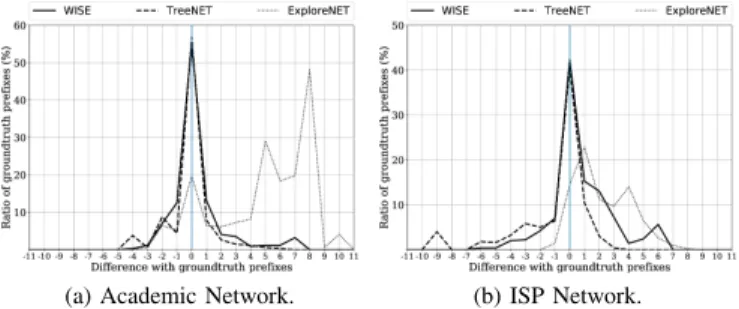
To validate WISE and compare its performance with the state of the art, we introduce the notion of subnet distance, computed as follows: for each subnet in the groundtruth, we look for similar subnets in our measurements, either identical or overlapping, and compute the difference in bits between the prefix lengths. A value of 0 in the subnet distance corresponds
10https://github.com/JefGrailet/WISE/tree/master/Evaluation/Validation
11For security and confidentiality concerns, we will not make our datasets
(a) Academic Network. (b) ISP Network. Fig. 3. Subnet distance of inferred subnets on our groundtruths.
to a perfect inference, meaning the inferred prefix perfectly fits the groundtruth. A subnet distance < 0 corresponds to overgrown subnets, while positive values refer to undergrown subnets. If we plot the ratios of groundtruth subnets over-lapping inferred subnets for each subnet distance (on the X axis), we expect the curve to be heavily centered around 0, suggesting thus the inference tool performs well with respect to the groundtruth.
In the presence of errors, it is worth noticing that we prefer subnet distance to be positive (i.e., undergrown subnets) for two reasons. First, the lack of live interfaces in a part of the subnet address space can simply prevent the inference of its true prefix length, and therefore, an undergrown subnet can still be faithful to the actual topology. For instance, a /24 subnet where only addresses in the first half are being used in practice will typically be revealed as a /25 by WISE. Overgrown subnets, on the other hand, typically spans over multiple actual subnets and therefore cannot be considered as sound with respect to the actual topology. Second, undergrown subnets that are consecutive with respect to the address space can be compared and post-processed to recover the true prefix. Fig. 3 provides the ratios of groundtruth subnets being overlapped by our inferred subnets with respect to the subnet distance for both our groundtruth networks. In particular, Fig. 3a focuses on the academic network, while Fig. 3b on the Belgian ISP. On both figures, WISE (plain line) is compared to TreeNET(dashed line) and ExploreNET (dotted line). The blue vertical line at subnet distance 0 is a marker for the perfect situation. Generally speaking, both figures show that WISE is able to reveal as much exact prefixes as TreeNET. In addition, when focusing on errors, WISE is capable of providing subnets for which the prefix length differs from the groundtruth by a single bit. Also, WISE generates more undergrown subnets (subnet distance > 0) and less overgrown subnets compared to TreeNET. As we explained earlier, this is a desirable result, as undergrown subnets can either still be a realistic estimation, or be merged with other undergrown subnets to recover the actual subnet. In other words, WISE manages to provide noticeably better results than TreeNET while being more careful when it comes to large subnets. Finally, subnets discovered by ExploreNET are mostly located at the right side of each figure, meaning it generates much more undergrown subnets than both WISE and ExploreNET. Such a result is not surprising: indeed, TreeNET was designed to refine subnets discovered by ExploreNET in order to
TreeNET WISE Academic network Execution time 54’33 21’38 Amount of probes 19,136 26,831 Belgian ISP Execution time 11:32’24 34’27
Amount of probes 290,949 278,329
TABLE I
PERFORMANCE OFTR E ENETANDWISE.
better identify larger subnets, which ExploreNET tends to chunk [10]. Finally, we note that both our groundtruths are good settings for TreeNET, as phenomena like flickering and warping are uncommon with them. In a less propitious setting, we expect TreeNET to output more aberrant results.
We also take a closer look at performance during the subnet inference step of each tool. Table I shows the execution time of both TreeNET and WISE on each network as well as the total amount of probes sent by each. In both situations, WISE completes subnet inference much faster than TreeNET, and this is especially true on a large network such as the Belgian ISP. Indeed, the subnet inference as performed by TreeNET required hours of execution while WISE only took about half an hour, mostly because TreeNET considers a single subnet at once in a given thread (the bigger the subnet, the slower the execution time), while WISE will use the same thread to probe and study multiple IP addresses at a steady rate. This being said, WISE is also clearly more intensive in terms of probing, mostly due to its way of scanning the target IP addresses and scheduling probing work (including re-probing of target IP addresses which could not be successfully scanned) to get all the data it needs for (offline) subnet inference as quickly as possible, but remains very reasonable. In the case of the Belgian ISP, WISE sent on average 135 probes per second, which amounts to 7,560 bytes of data, assuming our typical probe is an ICMP probe (around 32 bytes) encapsulated in an IP packet (which the header adds a 24 bytes overhead).
V. MEASUREMENTS IN THEWILD
We now discuss the data we collected in the wild using the PlanetLab testbed. We use this data to show that WISE can find a good amount of sound-looking subnets in the wild as well as to demonstrate that WISE is able to re-discover the same subnets in a target domain whatever the vantage point location used in a measurement campaign. Our full dataset is publicly available online.12
A. Subnet Soundness Rules
In the absence of a groundtruth to assess the measurements validity, we have to define criteria indicating whether a given subnet is sound or aberrant. Ideally, a subnet should be as close as possible to the ideal definition used by state-of-the-art tools, but we should let room for situations where distances towards pivots (TTL-wise) are not all equal. We therefore define 3 rules for ensuring the soundness of a subnet: the contra-pivot rule, the spread rule, and the outlier rule.
The contra-pivot rule simply states that an ideal subnet should feature at least one interface viewed as a contra-pivot, as a subnet lacking one could be only a part of a larger subnet.
The spread rule states that, in the presence of contra-pivots, these interfaces are either in minority for large subnets, either no more common than pivots for small subnets (i.e., the prefix length 29 or greater). Finally, a subnet fulfilling the outlier rule is simply a subnet containing no other interfaces than pivots and contra-pivots. A subnet satisfying the three rules is considered as sound, and if the TTL distances of the pivots are identical while the contra-pivot(s) is (are) found exactly one hop sooner, then the subnet satisfies the ideal definition of previous state-of-the-art subnet inference tools.
It is worth noting that revealing a given subnet prefix from different vantage points does not mean that the prefixes will meet exactly the same soundness rules. For instance, it is always possible that the subnet revealed from vantage point X features an outlier, while the same subnet revealed from vantage point Y will exhibit highly varying distances, making the contra-pivot interface detection difficult. Our rules are thus also a good indicator on how various vantage points (and, consequently, the different paths towards the targeted domain) can increase the difficulty of inferring a given subnet, due to (for instance) traffic engineering, as discussed in Sec. II. B. Measurement Methodology
Starting from December 28th, 2018 up to the end of Febru-ary 2019, we measured 27 different ASes of vFebru-arying sizes (from small stub ASes to large transit ASes covering roughly four millions of IP addresses) from the PlanetLab testbed. We fully measured each AS using a single PlanetLab node as a vantage point and repeated the measurements on a daily basis, with the exception of some large ASes (such as AS2497 and AS9198) that required up to two days of measurement to be entirely scanned. Just like our evaluation of trail issues discussed in Sec. II-C, we changed our vantage point at each measurement run to assess the effects of measuring a same target domain from different perspectives, implementing in practice a rotation of our vantage points. Our scripts for scheduling measurements are publicly available online. 13 C. Observations in the Wild
To assess the soundness of our measurements, we first plot the amount of subnets collected for a given AS over a given period of time and show how many of these subnets fulfill a certain amount of rules (as presented in Sec. V-A). As we measured 27 ASes and scheduled several campaigns, we only show here the most typical cases to elaborate on how WISE performs in the wild. Interested readers can refer to our public repository for additional results. 14
Fig. 4 shows our results for both AS6453 (Fig. 4a) and AS3257 (Fig. 4b). It gives the amounts of inferred subnets (bottom part of the figure) and their soundness as ratios (top part of the figure). Both figures were generated with data collected during the first half of February 2019. The first major result highlighted by these figures is that all subnets fulfill at least one rule, and a quick look at the data shows that most
13https://github.com/JefGrailet/WISE/tree/master/Dataset/Scripts 14https://github.com/JefGrailet/WISE/tree/master/Evaluation/Accuracy/ 02/02 03/02 04/02 06/02 08/02 09/02 10/02 11/02 12/02 13/02 0 25 50 75 100 % of subnets
3 rules 2 rules 1 rule None
02/02 03/02 04/02 06/02 08/02 09/02 10/02 11/02 12/02 13/02 Dataset 5000 10000 15000 # subnets (a) AS6453 02/02 03/02 04/02 06/02 08/02 09/02 10/02 11/02 12/02 13/02 0 25 50 75 100 % of subnets
3 rules 2 rules 1 rule None
02/02 03/02 04/02 06/02 08/02 09/02 10/02 11/02 12/02 13/02 Dataset 10000 20000 30000 # subnets (b) AS3257
Fig. 4. Subnets quantities (down) and soundness (up, in %) (February 2019).
03/02 04/02 06/02 08/02Dataset09/02 10/0211/02 12/02 13/02 5000
10000 15000
# subnets (w.r.t. 02/02)
Strictly persistent Persistent No equivalent
(a) AS6453 03/02 04/02 06/02 08/02Dataset09/02 10/0211/02 12/02 13/02 10000 20000 30000 # subnets (w.r.t. 02/02)
Strictly persistent Persistent No equivalent
(b) AS3257 Fig. 5. Persistence of subnets (February 2019).
of the time, this rule is the outlier rule. In other words, WISE is able to infer a large majority of subnets (above 95%) that are free of outliers, showing that its subnet inference is very careful and rarely produces aberrant subnets. The other result is that the amount of subnets fulfilling the three rules is also considerable, with several datasets having more than 60% of subnets fulfilling all rules in the case of AS6453. The ratios of subnets fulfilling only two rules is fairly low, however, but they all correspond to cases where there is at least one contra-pivot and where the presence of outliers or the amount of contra-pivot interfaces violates the outlier rule or the spread rule, respectively. Another interesting result is that WISE is rather constant in the soundness of its inference despite the highly varying difficulties encountered with the selected ASes (see Sec. II-C), though the ratio of sound subnets (i.e. fulfilling all rules) can sometimes have a sudden drop. Interestingly, this drop can correspond to situations where WISE discovered more subnets, as shown by Fig. 4b. As the amount of alive IP addresses did not change that much between datasets, this suggests the subnets discovered during previous measurement campaigns were actually chunked because of new difficulties induced by additional traffic engineering.
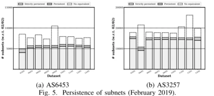
We also take a look at the persistence of subnets across various measurement runs. A subnet is said to be (weakly) persistentif its prefix is present in two datasets collected from different vantage points. It is said to be strictly persistent if both measurements fulfill the same amount of rules (defined in Sec. V-A). A weakly persistent subnet demonstrates two things: first, changing the vantage point from one run to another can lead to issues as described in Sec. II-C. This will worsen the quality of the dataset and make the measured subnet look less sound. Second, this shows WISE can recover the same subnets despite these issues to some extent.
before on the same dates, using each time the first collected dataset as reference dataset (i.e., all subsequent datasets are compared to this one). The results show that the subnets discovered by WISE have a good persistence overall, with a majority of strictly persistent subnets in both situations for most datasets. The noticeable amount of persistent subnets fulfilling a different amount of rules for each dataset shows, on the other hand, that each measurement comes with a certain amount of subnets that differs from previous measurements. An interesting observation to make is that the persistent sub-nets drop (both in the weak and the strict sense) on February 4th, 2019 for AS3257 correlates with the drop of subnets
fulfilling all rules on the same date (compare Fig. 4b and 5b). Moreover, the amount of subnets being weakly persistent is noticeably greater than for any other dataset, supporting so the idea that traffic engineering or measurement issues can both decrease the soundness of the measurement and cause previously measured subnets to appear differently as well. In particular, outliers can appear from one measurement to another, or warping interfaces can make the distances of both pivots and contra-pivots vary.
To give a practical example, one can look at the sub-net 129.242.88.0/21 WISE regularly discovered in AS224 (UNINETT). In most measurements, the subnet appears with a single contra-pivot and very regular distances (all pivots being located at the same TTL), a result that can be seen in the dataset collected on February 2nd, 2019. However, on February
8th and February 10th, the same subnet appeared with highly
varying TTLs for the pivots, with the former dataset having pivots at respectively 16 or 18 hops and the latter at 21 and 24 hops. Hopefully, the contra-pivot always appearing sooner, all measurements remain sound w.r.t. our usual criteria. All our figures and scripts to study the persistence of subnets are available in our public repository. 15
Overall, our measurements show that, while choosing the vantage point is still important to maximize accuracy of the subnet inference, a tool such as WISE can mitigate pretty well traffic engineering issues with a few exceptions. As we lack of space to show more figures, we encourage readers to take a look at our repository to see all figures. In particular, we also provide figures showing the distribution of subnet prefix lengths in our datasets.16These additional figures demonstrate WISE can discover all kinds of prefix length though the distribution of these lengths will usually follow a power-law shape (30 and 31 being the most common prefix lengths), as already pointed out previously in the literature [9].
VI. CONCLUSION
In this paper, we characterized and quantified measurement phenomena that can increase the difficulty of subnet inference, and introduced a new tool, WISE, which can detect and work around these issues without modifying the collected data. As our validation on simple groundtruth networks showed, WISE
15https://github.com/JefGrailet/WISE/tree/master/Evaluation/Persistence
16https://github.com/JefGrailet/WISE/tree/master/Evaluation/Prefixes
is perfectly able to compete with state-of-the-art tools in terms of subnet soundness but is also capable of outperforming them in terms of execution time, thanks to its design emphasizing linear complexity at all algorithmic steps.
Measurements in the wild with WISE showed that taking into account issues such as warping and flickering addresses can mitigate very well the effects of traffic engineering which vary from one vantage point to another, despite that some drastic changes can still occur from one vantage point to another. In other words, while selecting a good vantage point remains important, carefully designing subnet inference can mitigate rather well issues which depend on it. Further research into the selection of a good vantage point could be the next step for achieving subnet inference that is both accurate and efficient. It should also be noted that subnet post-processing as performed by WISE is still in its infancy, and that considering more possible scenarii could further improve inference.
REFERENCES
[1] B. Donnet and T. Friedman, “Internet topology discovery: a survey,” IEEE Communications Surveys and Tutorials, vol. 9, no. 4, December 2007.
[2] B. Augustin, X. Cuvellier, B. Orgogozo, F. Viger, T. Friedman, M. Lat-apy, C. Magnien, and R. Teixeira, “Avoiding traceroute anomalies with Paris traceroute,” in Proc. ACM Internet Measurement Conference (IMC), October 2006.
[3] B. Augustin, B. Krishnamurthy, and W. Willinger, “IXPs: Mapped?” in Proc. ACM Internet Measurement Conference (IMC), November 2009. [4] G. Nomikos and X. Dimitropoulos, “traIXroute: Detecting IXPs in
traceroute paths,” in Proc. Passive and Active Measurements Conference (PAM), April 2016.
[5] Y. Shavitt and N. Zilberman, “Geographical Internet PoP level maps,” in Proc. Traffic Monitoring and Analysis Workshop (TMA), March 2012. [6] D. Feldman, Y. Shavitt, and N. Zilberman, “A structural approach for PoP geo-location,” Computer Networks (COMNET), vol. 56, no. 3, pp. 1029–1040, February 2012.
[7] J. Mogul and J. Postel, “Internet standard subnetting procedure,” Internet Engineering Task Force, RFC 950, August 1985.
[8] M. E. Tozal and K. Sarac, “TraceNET: an Internet topology data collector,” in Proc. ACM Internet Measurement Conference (IMC), November 2010.
[9] M. E. Tozal and K. Sarac, “Subnet level network topology mapping,” in Proc. IEEE International Performance Computing and Communications Conference (IPCCC), November 2011.
[10] J.-F. Grailet, F. Tarissan, and B. Donnet, “TreeNET: Discovering and connecting subnets,” in Proc. Traffic and Monitoring Analysis Workshop (TMA), April 2016.
[11] B. Augustin, R. Teixeira, and T. Friedman, “Measuring load-balanced paths in the Internet,” in In Proc. ACM Internet Measurement Conference (IMC), October 2007.
[12] P. Mérindol, B. Donnet, O. Bonaventure, and J.-J. Pansiot, “On the impact of layer-2 on node degree distribution,” in Proc. ACM Internet Measurement Conference (IMC), November 2010.
[13] P. Marchetta, P. Mérindol, B. Donnet, A. Pescapé, and J.-J. Pansiot, “Quantifying and mitigating IGMP filtering in topology discovery,” in Proc. IEEE Global Communications Conference (GLOBECOM), December 2012.
[14] J.-F. Grailet and B. Donnet, “Towards a renewed alias resolution with space search reduction and ip fingerprinting,” in Proc. Network Traffic Measurement and Analysis Conference (TMA), June 2017.
[15] Y. Vanaubel, J.-J. Pansiot, P. Mérindol, and B. Donnet, “Network fingerprinting: TTL-based router signatures,” in Proc. ACM Internet Measurement Conference (IMC), October 2013.
[16] N. Spring, R. Mahajan, and D. Wetherall, “Measuring ISP topologies with Rocketfuel,” in Proc. ACM SIGCOMM, August 2002.
[17] K. Keys, “iffinder,” a tool for mapping interfaces to routers. See http: //www.caida.org/tools/measurement/iffinder/.