HAL Id: hal-01666536
https://hal.archives-ouvertes.fr/hal-01666536
Submitted on 18 Dec 2017
HAL is a multi-disciplinary open access
archive for the deposit and dissemination of
sci-entific research documents, whether they are
pub-lished or not. The documents may come from
teaching and research institutions in France or
abroad, or from public or private research centers.
L’archive ouverte pluridisciplinaire HAL, est
destinée au dépôt et à la diffusion de documents
scientifiques de niveau recherche, publiés ou non,
émanant des établissements d’enseignement et de
recherche français ou étrangers, des laboratoires
publics ou privés.
promoting criteria
Marc Castella, Jean-Christophe Pesquet
To cite this version:
Marc Castella, Jean-Christophe Pesquet. A global optimization approach for rational sparsity
pro-moting criteria. EUSIPCO 2017 - 25th European Signal Processing Conference, Aug 2017, Kos Island,
Greece. pp.156 - 160, �10.23919/EUSIPCO.2017.8081188�. �hal-01666536�
A Global Optimization Approach for Rational
Sparsity Promoting Criteria
Marc Castella
SAMOVAR, T´el´ecom SudParis, CNRS, Universit´e Paris-Saclay,
9 rue Charles Fourier, 91011 Evry Cedex, France Email: [email protected]
Jean-Christophe Pesquet
Center for Visual Computing, CentraleSupelec, Universit´e Paris-Saclay,
Grande Voie des Vignes, 92295, Chˆatenay-Malabry, France Email: [email protected]
Abstract—We consider the problem of recovering an unknown
signal observed through a nonlinear model and corrupted with additive noise. More precisely, the nonlinear degradation consists of a convolution followed by a nonlinear rational transform. As a prior information, the original signal is assumed to be sparse. We tackle the problem by minimizing a least-squares fit criterion penalized by a Geman-McClure like potential. In order to find a globally optimal solution to this rational minimization problem, we transform it in a generalized moment problem, for which a hierarchy of semidefinite programming relaxations can be used. To overcome computational limitations on the number of involved variables, the structure of the problem is carefully addressed, yielding a sparse relaxation able to deal with up to several hundreds of optimized variables. Our experiments show the good performance of the proposed approach.
I. INTRODUCTION
Over the last decade, much attention has been paid to inverse problems involving sparse signals. A popular approach for solving such problems consists in minimizing the sum of a data fidelity term and a regularization term incorporating prior information. When the observation model is linear and the noise has a log-concave likelihood, a convex cost function is obtained. Many efforts have then been dedicated to derive efficient algorithms able to deal with a large number of variables, while ensuring convergence to a global minimizer [1]–[3]. As we will explain now, such a convex formulation may however be limited for two main reasons.
Firstly, for many real acquisition devices, the actual degra-dation model is not linear and some nonlinear saturation effects often arise. A simplified model then results from a linearization procedure which overlooks these nonlinear be-haviors in order to make the associated mathematical problem tractable. For example, standard tools in signal processing such as the Wiener filter are effective mostly in a linear framework. For a long time, attempts have been made in order to deal with more general nonlinear models. For example, one can mention the works undertaken by using Volterra models [4], which may be useful in some application areas [5]. Secondly, convex regularization terms may be limited, especially for capturing the sparse structure of a signal. Potentials related to the ℓ1norm are often employed as surrogates to the natural sparsity measure, which is the ℓ0 pseudo-norm (count of the number of nonzero components in the signal). Although
some theoretical works have promoted the use of the ℓ1 norm [6], its optimality can only been established under some restrictive assumptions. In turn, cost functions involving the
ℓ0pseudo-norm lead to NP-hard problems for which reaching a global minimum cannot be guaranteed in general [7]–[9]. Smooth approximations of the ℓ0 pseudo-norm may appear as good alternative solutions [10]–[13]. However, for most of the existing optimization algorithms (e.g. those based on Majorize-Minimize strategies), only convergence to a local minimum can be expected. One can however mention the recent work in [14] where a Geman-McClure like potential was used for deconvolving a sparse signal. Promising results were then obtained.
In this work, we extend the scope of our preliminary work in [14] by proposing a novel approach for restoring sparse signals degraded by a nonlinear model. More precisely, our contributions in this paper are threefold. First, the proposed approach is able to deal with degradation models consisting of a convolution followed by a pointwise transform. The latter appears as a rational fraction involving absolute values and, as an extension of [14], real-valued quantities are here allowed. Such nonlinearly distorted convolution models may also be encountered in blind source separation [15] and neural networks [16]. Our second contribution is to allow the use of a Geman-McClure like regularization with proven global con-vergence guaranties to a solution of the associated optimization problem. The last contribution of this work is to devise a sparse relaxation in the spirit of [17] to cope with the resulting rational optimization. Since these general rational optimization methods are grounded on building a hierarchy of semidefinite programs (SDP), such a relaxation plays a prominent role in making these approaches applicable to several hundred of variables as it is common in inverse problems.
In Section II, we state our nonlinear model and define the optimized criterion. Section III describes the main steps of our approach. Section IV provides simulation results and Section V concludes this paper. The set of polynomials in the indeterminates given by vector x := (x1, . . . , xT) is denoted
II. MODEL AND CRITERION
A. Sparse signal model
We consider the problem of recovering a set of unknown samples given by the vector x := (x1, . . . , xT)⊤. In our
context, we only have access to some measurements related to the original signal through a linear transformation (typically, a convolution) and some nonlinear effects. More precisely, the observation model reads
y = ϕ(Hx) + n , (1) where the vector y := (y1, . . . , yT)⊤ contains the observation
samples, n := (n1, . . . , nT)⊤ is a realization of a random
independently and identically distributed (i.i.d.) noise vector,
H ∈ RT×T is a given matrix, and ϕ : RT → RT is a
nonlinear function. For simplicity, it is assumed that ϕ applies componentwise, that is, for every u := (u1, . . . , uT)⊤, the
k-th component of ϕ(u) is given by [ϕ(u)]k = ϕ(uk). Here, ϕ
models a rational saturation effect, which is parametrized by
δn> 0, and which is given by:
(∀u ∈ R) ϕ(u) = u
δn+|u|
. (2)
The model (1) appears in the case when the samples stem from a signal given by yt= ϕ(ht⋆ xt) + ntfor all t∈ {1, . . . , T }.
In the latter equation, ⋆ denotes the convolution by the filter with impulse response (ht)t. We assume that the convolution
filter has a finite impulse response (FIR) given by the vector (h1, . . . , hL)⊤. Under suitable vanishing boundary conditions,
the matrix H is thus Toeplitz banded as shown below:
H = h1 0 ... ... ... 0 .. . . ... .. ... hL . .. ... 0 . .. . .. ... .. . . .. ... . .. 0 0 ... 0 hL ... h1 .
One of the main novelty of this work is to exploit the spe-cific structure of matrix H in order to reduce the computational cost of the subsequently proposed global optimization method. Finally, the signal (xt)t∈Z is assumed to be sparse, that is we
simply assume that xt̸= 0 only for a few indices t.
B. Criterion for recovery
Following a classical approach for estimating x, we mini-mize a penalized criterion having the following form:
(∀x ∈ RT) J (x) = ∥y − ϕ(Hx)∥2+ λ
T
∑
t=1
ψδ(xt) , (3)
where λ and δ are positive regularization and smoothing parameters, and ψδ is a Geman-McClure like potential similar
to the one used in [14]:
(∀ξ ∈ R) ψδ(ξ) =
|ξ|
δ +|ξ|. (4)
The minimization is performed over a compact feasible set denoted by K and the optimization problem consists in finding
J⋆:= inf
x∈KJ (x) .
III. RATIONAL MINIMIZATION
To solve J⋆, we use a methodology similar to [14]. The
differences and novelties are described in the next two sub-sections: first, we can deal with real-valued quantities, and second, we exploit the problem structure.
A. Optimization set and absolute values
We here specify the feasible set K. From its description, it becomes possible to cope with the absolute values in (2) and (3). First, the optimization set K mentioned above is described by polynomial inequalities as follows:
K ={x ∈ RT| gi(x)≥ 0, i = 1, . . . , I}. (5)
Technically, it is required that the above representation of
K provides an algebraic certificate of compactness [18]. In
our practical situation, this is easily satisfied when upper and lower bounds on the variables (xt)1≤t≤T are available: in this case indeed, K⊂ [−B, B]T and hence the polynomials corre-sponding to the inequalities gt(xt) =−(xt+ B)(xt− B) ≥ 0
can be included in the polynomials in (5). Details on these technical conditions are out of the scope of this paper and can be found in [18, 19].
Furthermore, we can use the above specification of the feasible set K to handle absolute values. First, by introducing a polynomial and its opposite in (5), it is possible to introduce polynomial equality constraints in K. Then, absolute values can be considered as follows: for each term|˜u(x)| appearing, where ˜u is a polynomial, add an additional variable u and
impose the constraints u≥ 0, u2= ˜u(x)2. The methodology described in Section III-C of this paper can then be applied with the extended set of variables (x, u).
B. Structure of the problem
Developing the square norm in (3) and substituting all terms, the criterionJ appears as a sum of rational functions, possibly involving absolute values. The absolute values can be eliminated using the trick of the previous paragraph: for clarity, and with no loss of generality, we describe the method when all quantities are nonnegative and hence no absolute values appear.
We take advantage of the Toeplitz banded structure of H, and introduce a sparse1 relaxation of J⋆. This technique
was introduced in a different context [17]. Define for each
t ∈ {1, . . . , T } the set It = {min{1, t − L + 1}, . . . , t} of
1The notion of sparsity here concerns the SDP relaxation and should not
column indices of H for which row t has nonzero elements. Developing the square norm in (3), we writeJ (x) as follows:
J (x) = T ∑ t=1 [ yt− ϕ ( L ∑ i=1 hixt−i+1 )]2 | {z } pIt (x) qIt (x) + λψδ(xt) | {z } p(xt) q(xt) ,
with the convention that xt = 0 for t /∈ {1, . . . , T }. In other
words, pIt, qIt are polynomials that depend on the variables (xk)k∈It only and p, q are univariate polynomials that depend on xt only. Define the following sets:
(∀t ∈ {1, . . . , T }) Jt= Itand Jt+T ={t} .
The sets (Jt)1≤t≤2T satisfy ∪2T
t=1Jt={1, . . . , T } and the
so-called Running Intersection Property (RIP), that is for every
t∈ {2, . . . , 2T }: Jt ∩(t∪−1 k=1 Jk ) ⊆ Jj for some j≤ t − 1 .
Consequently, the methodology in [17] is applicable.
C. Sparse SDP relaxation
Similarly to [14], J⋆ can be relaxed to a finite
dimen-sional SDP, where each optimization variable corresponds to a monomial in (x1, . . . , xT). We briefly sketch the main
steps. First, it can be proved that the original problem is equivalent to an optimization problem over several finite Borel measures, which is called a generalized moment problem. Each measure is then represented by a truncated moment sequence y. For any such moment sequence, we define the following linear functional, which replaces any monomial in a given polynomial f ∈ R[x] by the corresponding moment value in y:
Ly: R[x] → R
f =∑fαxα7→ ∑
fαyα.
In the relaxation below, Ly(f ) will correspond to the value
taken by a polynomial f for a given measure represented by the moment sequence y. For any order k ∈ N and for multi-indices α, β of order |α| := α1+· · · + αn ≤ k and |β| ≤ k,
the moment matrix of y is defined by [Mk(y)]α,β := yα+β,
and for a given polynomial g ∈ R[x], the localizing matrix associated with g and y is
[Mk(gy)]α,β:= ∑
γ
gγyγ+α+β.
The two above matrices, will make it possible in the relax-ation to introduce the conditions such as Mk(y) ⪰ 0 and
Mk(gy)⪰ 0, which are necessary for y to represent a measure
concentrated on the set where g is nonnegative. Finally, the
kth order sparse SDP relaxation consists in the minimization problem P⋆s k := inf T ∑ t=1 Lzt(pIt) + Lyt(p)
subject to a number of semidefinite positivity constraints and linear equality constraints (see [17] for mathematical details). Note in particular that, in order to deal with the fractions in J (x), the constraints Lzt(qIt) = Lyt(q) = 1 on the denominator values should appear.
With increasing values of k, this yields a hierarchy of SDP relaxations for which it can be proved [17] thatPk⋆s↑ J⋆ as
k → ∞. Moreover, from Pk⋆s, a point x⋆sk can be extracted, which is guaranteed to be optimal under certain rank condi-tions and possibly only approximate otherwise.
The above relaxation is similar to the one in [14]. Based on the split form ofJ (x), the moment sequences ytcorrespond
to monomials involving the variables (xk)k∈Jt which appear in the respective terms pIt(x)
qIt(x). Similarly, the moment sequences
ztcorrespond to monomials involving xtonly, in accordance
to the variable appearing in the terms p(xt)
q(xt). Of course, the same subset of variables may appear in different moment sequences yt or zt: therefore compatibility conditions are
required, corresponding to equality of moments. This is made possible by the RIP condition and it justifies that linear equality constraints are necessary inP⋆s.
Importantly, and in contrast with [14], no moment sequence involves all variables (xt)1≤t≤T. As a consequence, the semi-definite positivity constraints inP⋆s
k only involve small subsets
of the whole set of variables (xt)1≤t≤T. This constitutes the great benefit of this sparse relaxation, allowing us to deal with a much higher number of variables. A striking example illustrating this fact is when the criterion is separable and the terms inJ (x) all involve distinct variables.
IV. SIMULATIONS
A. Experimental setup
We have generated samples x from a sparse signal. The number of samples in x has been set to T = 200, T = 100,
T = 50 and T = 20. We have imposed that exactly 10% of
the samples are nonzero, yielding respectively 20, 10, 5 and 2 nonzero components in x. The amplitudes of the nonzero components have been drawn according to a uniform distribu-tion on [−1; −2/3] ∪ [2/3; 1]. Then, this unknown impulsive signal has been corrupted according to Model (1) with the nonlinearity given by (2). We have set δn= 0.3 and the noise
n has been drawn according to an i.i.d. zero-mean Gaussian
distribution with standard deviation σ = 0.15. Finally, the matrix H has been set Toeplitz banded corresponding to FIR filters of length 3. Several sets of 100 Monte-Carlo realizations of such data have been generated, both with fixed FIR filter with impulse responses given by h(a)= [0.1, 0.8, 0.1] and by
h(b)= [0.3871,−0.1887, 0.4242] and with impulse responses drawn randomly for each Monte-Carlo realization. We have set empirically λ = 0.15 for the regularization parameter and
δ = 0.01 in the penalty function (4). To obtain an estimate x⋆s
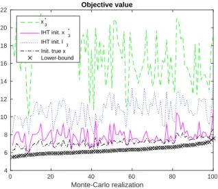
Monte-Carlo realization 0 20 40 60 80 100 4 6 8 10 12 14 16 18 20 22 Objective value x 3 * IHT init. x3* IHT init. l 1 Init. true x Lower-bound
Fig. 1. For all realizations, lower bound and objective value attained by our method; objective value attained by IHT with different initializations (filter with random coefficient, T = 200).
we have solved the SDP relaxation P3⋆s of order k = 3 from Section III-C. We are not aware of any other method able to find the global minimum of (3) and for comparison, we have used a linearized model: for reconstruction purposes, using data generated according to (1), we have linearized around zero the nonlinearity in (2) and have used the well-known ℓ1 penalization.
Finally, we have also implemented a proximal gradient algorithm based on Iterative Hard Thresholding (IHT) [8] extended to the nonlinear model. The latter algorithm however only certifies convergence to a local minimum of the criterion. Due to non convexity, the local minima are likely to be different from the global minimum.
B. Performance of the proposed relaxation
Note first that, for the order of relaxation k = 3, we have been able to consider up to T = 200 samples with the sparse relaxation used here. This is a significant improvement in comparison with the results in [14], where the relaxation was able to deal with only a few tens of variables with an order of relaxation not greater than 3.
We have plotted on Figure 1 the lower bound provided by the relaxation P3⋆s and the objective value J (x⋆s3) at-tained when extracting an optimal point from the same order relaxation. We clearly see that P⋆s
3 ≤ J (x⋆s3 ), which is in accordance with the theory. However, equality does not perfectly hold. This illustrates that the choice k = 3 of the relaxation order is probably too small for the considered problem. As a consequence, we propose in next section to combine our method with a local IHT optimization method.
C. Existence of local minima and results of the proposed global approach
The IHT algorithm has been initialized with x⋆s3 , the result from the linearized model and ℓ1 penalization, y, an
all-zero vector and the true x (the latter initialization would be intractable in real applications). The average values over all Monte-Carlo realizations are provided in Table I for T = 200. Some detailed values, corresponding to randomly drawn filter coefficients, are plotted in Figure 1, also for T = 200.
The final objective values after convergence of the IHT optimization clearly depend on the initialization, which ad-vocates in favor of the existence of several local optima and emphasizes the importance of considering the problem of global optimization. In average, the lowest objective value is obtained by a local optimization initialized either at x⋆s
3 or at the true x. More importantly, as shown in Table II, the IHT algorithm seems unable to reach the global minimum with any of the initializations easily available (ℓ1, y, all-zero vector). This shows clearly that the proposed relaxation is very useful in providing an improved initialization point for a local optimization algorithm.
TABLE I
FINAL VALUES OF THE OBJECTIVEJ (x)FOR THE NONLINEAR LOCAL
OPTIMIZATION METHODS.
Opt. method Filter param.
h(a) h(b) random x⋆s 3 12.181 20.852 16.776 linearized ℓ1 22.032 19.719 20.848 IHT, init. x⋆s 3 7.2900 8.9858 7.8665 IHT, init. ℓ1 10.157 11.186 10.690 IHT, init. y 10.167 12.505 13.144 IHT, init. zero 12.231 15.417 13.392 IHT, init. x 7.1992 7.1578 7.1489
TABLE II
OUT OF100 MONTE-CARLO REALIZATIONS,NUMBER OF TIMES EACH
INITIALIZATION OFIHTPROVIDES THE SMALLEST OBJECTIVE VALUE
(FILTERh(a), T = 200). Num. samples Initialization x⋆s 3 ℓ1 y zero x 20 56 0 1 18 40 50 38 0 0 0 62 100 36 0 0 0 64 200 22 0 0 0 78
D. Results on signal recovery
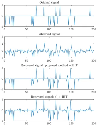
Finally, we illustrate the ability of our method to estimate the sought signal. A typical example of the true x, of the observation vector y and of the reconstructed signal is given on Figure 2. The estimation error on x has been quantified by the mean square error 1
T∥ˆx − x∥
2 for a given estimate ˆx. The average error and objective values are gathered in Table III and show poor results are obtained with a linearized model. The best results have been obtained by IHT initialized by x⋆s
3. The result of IHT initialized by the true x is given for information.
V. CONCLUSION
We have considered sparse signals observed through a nonlinear observation model with additive noise. The class of nonlinear models that can theoretically be tackled with our methodology is quite vast, as it includes any rational function, possibly involving absolute values.
0 50 100 150 200 -1 0 1 Original signal 0 50 100 150 200 -1 0 1 2 Observed signal 0 50 100 150 200 -1 0 1
Recovered signal: proposed method + IHT
0 50 100 150 200
-1 0 1
Recovered signal: ℓ1+ IHT
Fig. 2. Typical original signal x, observations y and recovered signal. The results presented have been obtained with IHT initialized either by our method or by a linearized model and ℓ1 penalty.
TABLE III
FINAL AVERAGEMSEFOR THE NONLINEAR LOCAL OPTIMIZATION
METHODS.
Opt. method Filter param.
h(a) h(b) random
x⋆s
3 8.40e-3 1.57e-2 1.29e-2
linearized ℓ1 3.88e-2 3.15e-2 3.38e-2
IHT, init. x⋆s3 8.95e-3 1.45e-2 1.22e-2
IHT, init. ℓ1 1.30e-2 2.14e-2 1.95e-2
IHT, init. y 2.60e-2 2.34e-2 3.96e-2 IHT, init. zero 5.20e-2 6.60e-2 5.57e-2 IHT, init. x 5.18e-3 4.08e-3 4.49e-3
The starting point of our reconstruction approach involves the minimization of a criterion which is the sum of a fidelity term and a penalization. The fidelity has been chosen as a square norm and the penalization as a Geman-McClure potential approaching the ℓ0norm. It has been known for long that such problems are particularly hard to solve. However, with the adopted formulation and approximation, the optimiza-tion problem is raoptimiza-tional, which opens up the possibility to use recent methodologies with theoretical global convergence properties.
The desirable convergence properties of the latter method-ologies come at the cost of solving a high dimensional SDP. With state of the art SDP solvers, this limits the approach to small size problems. To overcome these computational
limitations, we have exploited a particular model structure. In so doing, we have been able to deal with up to 200 variables. More specifically, the proposed methodology seems promising in order to provide an initialization point to a local algorithm such as IHT. Finally, the results in terms of reconstruction seem promising.
REFERENCES
[1] P. L. Combettes and J.-C. Pesquet, “Proximal splitting methods in signal processing,” in Fixed-Point Algorithms for Inverse Problems in Science and Engineering, H. H. Bauschke, R. Burachik, P. L. Combettes, V. Elser, D. R. Luke, and H. Wolkowicz, Eds. New York: Springer-Verlag, 2010, pp. 185–212.
[2] N. Komodakis and J.-C. Pesquet, “Playing with duality: an overview of recent primal-dual approaches for solving large-scale optimization problems,” IEEE Signal Process. Mag., vol. 32, pp. 31–54, Nov. 2015. [3] S. Boyd, N. Parikh, E. Chu, B. Peleato, and J. Eckstein, “Distributed optimization and statistical learning via the alternating direction method of multipliers,” Found. Trends Machine Learn., vol. 8, no. 1, pp. 1–122, 2011.
[4] M. Shetzen, The Volterra and Wiener Theories of Nonlinear Systems. New York: Wiley and sons, 1980.
[5] N. Dobigeon, J.-Y. Tourneret, C. Richard, J. C. M. Bermudez, S. McLaughlin, and A. O. Hero, “Nonlinear unmixing of hyperspectral images: models and algorithms,” IEEE Signal Process. Mag., vol. 31, no. 1, pp. 82–94, Jan. 2014.
[6] E. J. Cand`es and M. B. Wakin, “An introduction to compressive sampling,” IEEE Signal Process. Mag., vol. 25, no. 2, pp. 21–30, Mar. 2008.
[7] M. Nikolova, “Description of the minimizers of least squares regularized with ℓ0norm. Uniqueness of the global minimizer,” SIAM J. Imaging
Sci., vol. 6, no. 2, pp. 904–937, 2013.
[8] T. Blumensath and M. E. Davies, “Iterative thresholding for sparse approximations,” J. Fourier Anal. Appl., vol. 14, no. 5-6, pp. 629–654, 2008.
[9] A. Patrascu and I. Necoara, “Random coordinate descent methods for ℓ0
regularized convex optimization,” IEEE Trans. Automat. Contr., vol. 60, no. 7, pp. 1811–1824, Jul. 2015.
[10] S. Geman and D. McClure, “Bayesian image analysis: An application to single photon emission tomography,” in Proc. Statist. Comput. Section Amer. Statist. Association, 1985, pp. 12–18.
[11] E. Chouzenoux, A. Jezierska, J.-C. Pesquet, and H. Talbot, “A majorize-minimize subspace approach for ℓ2-ℓ0 image regularization,” SIAM J.
Imaging Sci., vol. 6, no. 1, pp. 563–591, 2013.
[12] A. Florescu, E. Chouzenoux, J.-C. Pesquet, P. Ciuciu, and S. Ciochina, “A majorize-minimize memory gradient method for complex-valued inverse problem,” Signal Process., vol. 103, pp. 285–295, Oct. 2014, special issue on Image Restoration and Enhancement: Recent Advances and Applications.
[13] E. Soubies, L. Blanc-F´eraud, and G. Aubert, “A continuous exact ℓ0
penalty (CEL0) for least squares regularized problem,” SIAM J. Imaging Sci., vol. 8, no. 3, pp. 1607–1639, 2015.
[14] M. Castella and J.-C. Pesquet, “Optimization of a Geman-McClure like criterion for sparse signal deconvolution,” in Proc. IEEE Int. Workshop on Computational Advances in Multi-Sensor Adaptive Processing (CAM-SAP), Cancun, Mexico, Dec. 2015, pp. 317–320.
[15] Y. Deville and L. T. Duarte, “An overview of blind source separation methods for linear-quadratic and post-nonlinear mixtures,” in Proc. of the 12th Int. Conf. LVA/ICA, ser. LNCS, vol. 9237. Liberec, Czech Republic: Springer, 2015, pp. 155–167.
[16] D. J. C. MacKay, Information Theory, Inference, and Learning Algo-rithms. Cambridge University Press, 2003.
[17] F. Bugarin, D. Henrion, and J.-B. Lasserre, “Minimizing the sum of many rational functions,” Mathematical Programming Computations, vol. 8, no. 1, pp. 83–111, 2015.
[18] J.-B. Lasserre, Moments, Positive Polynomials and Their Applications, ser. Optimization Series. Imperial College Press, 2010, vol. 1. [19] M. Laurent, “Sum of squares, moment matrices and optimization over
polynomials,” in Emerging Applications of Algebraic Geometry, ser. IMA Volumes in Mathematics and its Applications, M. Putinar and S. Sullivant, Eds. Springer, 2009, vol. 149, pp. 157–270.