Summarizing Semantic Graphs: A Survey

HAL Id: hal-01925496

https://hal.inria.fr/hal-01925496

Submitted on 16 Nov 2018

HAL is a multi-disciplinary open access

archive for the deposit and dissemination of

sci-entific research documents, whether they are

pub-lished or not. The documents may come from

teaching and research institutions in France or

L’archive ouverte pluridisciplinaire HAL, est

destinée au dépôt et à la diffusion de documents

scientifiques de niveau recherche, publiés ou non,

émanant des établissements d’enseignement et de

recherche français ou étrangers, des laboratoires

Summarizing Semantic Graphs: A Survey

Sejla Cebiric, François Goasdoué, Haridimos Kondylakis, Dimitris Kotzinos,

Ioana Manolescu, Georgia Troullinou, Mussab Zneika

To cite this version:

Sejla Cebiric, François Goasdoué, Haridimos Kondylakis, Dimitris Kotzinos, Ioana Manolescu, et al..

Summarizing Semantic Graphs: A Survey. The VLDB Journal, Springer, 2019, 28 (3). �hal-01925496�

Summarizing Semantic Graphs: A Survey

ˇ

Sejla ˇ

Cebiri´

c

_{Fran¸cois Goasdou´}

_e

_{Haridimos Kondylakis}

_{Dimitris Kotzinos}

Ioana Manolescu

Georgia Troullinou

Mussab Zneika

1

Inria and LIX (UMR 7161, CNRS and Ecole polytechnique), France2U. Rennes, Inria, CNRS, IRISA, France

3

ICS-FORTH, Greece 4ETIS, UMR 8051, U. Cergy-Pontoise, ENSEA, CNRS, France

November 15, 2018

Abstract

The explosion in the amount of the available RDF data has lead to the need to explore, query and un-derstand such data sources. Due to the complex structure of RDF graphs and their heterogeneity, the exploration and understanding tasks are signifi-cantly harder than in relational databases, where the schema can serve as a first step toward understand-ing the structure. Summarization has been applied to RDF data to facilitate these tasks. Its purpose is to extract concise and meaningful information from RDF knowledge bases, representing their content as faithfully as possible. There is no single concept of RDF summary, and not a single but many approaches to build such summaries; each is better suited for some uses, and each presents specific challenges with respect to its construction. This survey is the first to provide a comprehensive survey of summarization method for semantic RDF graphs. We propose a tax-onomy of existing works in this area, including also some closely related works developed prior to the adoption of RDF in the data management commu-nity; we present the concepts at the core of each ap-proach and outline their main technical aspects and implementation. We hope the survey will help read-ers undread-erstand this scientifically rich area, and iden-tify the most pertinent summarization method for a variety of usage scenarios.

1

Introduction

Semantic languages and models are increasingly used in order to describe, represent and exchange data in multiple domains and forms. In particular, given the prominence of the World Wide Web Consortium (W3C)1 _{in the international technological arena, its} standard model for representing semantic graphs, namely RDF, has been widely adopted. Many RDF Knowledge Bases (KBs, in short) of millions or even billions of triples are now shared through the Web, also thanks to the development of the Open Data movement, which has evolved jointly with the data linking best practices based on RDF. A famous repos-itory of open RDF graphs is the Linked Open Data cloud, currently referencing more than 62 billion RDF triples, organized in large and complex RDF data graphs [88]. Further, several RDF graphs are con-ceptually linked together into one, as soon as a node identifier appears in several graphs. This enables querying KBs together, and increases the need to un-derstand the basic properties of each data source be-fore figuring out how they can be exploited together. The fundamental difficulty toward understanding an RDF graph is its lack of a standard structure (or schema), as RDF graphs can be very heterogeneous and the basic RDF standard does not give means to constrain graph structure in any way. Ontologies can (but do not have to) be used in conjunction to RDF

data graphs, in order to give them more meaning, notably by describing the possible classes resources may have, their properties, as well as relationships between these classes and properties. On one hand, ontologies do provide an extra entry point into the data, as they allow to grasp its conceptual structure. On the other hand, they are sometimes absent, and when present, they can be themselves quite complex, growing up to hundreds or thousands of concepts; SNOMED-CT2_{, a large medical ontology, comprises} millions of terms.

To cope with these layers of complexity, RDF graph summarization has aimed at extracting con-cise but meaningful overviews from RDF KBs, repre-senting as close as possible the actual contents of the KB. RDF summarization has been used in multiple application scenarios, such as: identifying the most important nodes, query answering and optimization, schema discovery from the data, or source selection, and graph visualization to get a quick understand-ing of the data. It should be noted that indexunderstand-ing, query optimization and query evaluation were stud-ied as standalone problems in the data management areas, before the focus went to semantic RDF graphs; therefore, several summarization methods initially studied for data graphs were later adapted to RDF. Among the currently known RDF summarization ap-proaches, some only consider the graph data without the ontology, some others consider only the ontology, finally some use a mix of the two. Summarization methods rely on a large variety of concepts and tools, comprising structural graph characteristics, statis-tics, pattern mining or a mix thereof. Summarization methods also differ in their usage scope. Some sum-marize an RDF graph into a smaller one, allowing some RDF processing (e.g., query answering) to be applied on the summary (also). The output of other summarization methods is a set of rules, or a set of frequent patterns, an ontology etc.

Summarizing semantic graphs is a multifaceted problem with many dimensions, and thus many algo-rithms, methods and approaches have been developed to cope with it. As a result, there is now a confusion in the research community about the terminology in

2_{https://www.snomed.org/snomed-ct}

the area, further increased by the fact that certain terms are often used with different meanings in the relevant literature, denoting similar, but not identical research directions or concepts. We believe that this lack of terminology and classification hinders scien-tific development in this area.

To improve understanding of this field and to help students, researchers or practitioners seeking to iden-tify the summarization algorithm, method or tool best suited for a specific problem, this survey at-tempts to provide a first systematic organization of knowledge in this area. We propose a taxonomy of RDF (and most representative, prior graph) summa-rization approaches. Then, we classify existing works according to the main class of algorithmic notions they are based on; further, for each work, we specify their accepted inputs, outputs, and when a tool is publicly available, we provide the reference to it. We place each of the works in the space defined by the dimensions of our classification; we summarize their main concepts and compare them when appropriate. Since our focus is on RDF graph summarization techniques, we leave out of our scope graph sum-marization techniques tailored for other classes of graphs, e.g., biological data graphs [90], social net-works [57] etc. We focus on techniques that have either been specifically devised for RDF, or adapted to the task of summarizing RDF graphs. The litera-ture comprises surveys on generic (non-RDF) graph summarization, and/or partial surveys related to our area of study. The authors of [113] present generic graph summarization approaches, with a main focus on grouping-based methods. A recent survey [59] has a larger focus than ours. It considers static graphs as well as graphs changing over time; graphs which are just connection networks (node and edge labels are non-existent or ignored), but also labeled directed or undirected graphs, which can be seen as simple sub-sets of RDF. Also, a recent tutorial [40] covers a sim-ilar set of topics. However, given their broad scope, these works describe areas of work we are not con-cerned with, such as social (network) graph summa-rization, and ignore many of the proposals specifically tailored for RDF graphs, which are labeled, oriented, heterogeneous, and may be endowed with type infor-mation and semantics. In contrast, our survey seeks

to answer a need we encountered among many Se-mantic Web practitioners, for a comprehensive review of summarization techniques tailored exactly to such graphs. Another recent work [80] focuses on metrics used for ontology summarization only, whereas we consider both RDF graphs and their ontologies.

Our survey is structured as follows: Section 2 re-calls the foundations of the RDF data model, and RDF Schema (RDFS, in short), the simplest ontology language which can be used in conjunction with RDF to specify semantics for its data. Section 3 describes RDF summarization scope, applications and dimen-sions of analysis for this survey. In Section 4, we classify along these dimensions a selection of the main graph summarization works which preceded works on RDF summarization. We include a short discussion of these works here, as they were the first to intro-duce a set of concepts crucial for summarization, and on which RDF-specific summaries have built. In the sequel of the survey, Sections 5, 6, 7 and 8 analyze the related works in each category. Finally, Section 9 concludes this paper and identifies fields of future ex-ploration.

2

Preliminaries: RDF graphs

We recall here the core concepts and notations related to RDF graphs. At a first glance, these can be con-sidered particular cases of labeled, oriented graphs, and indeed classical graph summarization techniques have been directly adapted to RDF; we recall them in Section 2.1. Then, we present RDF graphs in Sec-tion 2.2, where we introduce the terminology and spe-cific constraints which make up the RDF standard, established by the W3C; we also introduce here on-tologies, which play a central role in most RDF ap-plications, with a focus on the simple RDF Schema ontology language. From a database perspective, the most common usage of RDF graphs is through queries; therefore, we recall the Basic Graph Pattern (BGP) dialect at the core of the SPARQL RDF query language in Section 2.3. Finally, a brief discussion of more expressive ontology languages, sometimes used in conjunction with RDF graphs, is provided in Sec-tion 2.4.

2.1

Labeled directed graphs:

core

concepts

Labeled directed graphs are the core concept allowing to model RDF datasets. Further, most (not all) pro-posals for summarizing an RDF graph also model the summary as a directed graph. Thus, without loss of generality, we will base our discussion on this model. Note that it can be easily generalized to more com-plex graphs, e.g., those with (multi-)labeled nodes.

Given a set A of labels, we denote by G = (V, E) an A-edge labeled directed graph whose vertices are V , and whose edges are E ⊆ V × A × V .

Figure 1 displays two such graphs; A edge la-bels are attached to edges. Node labels will be used/explained shortly in our discussion.

Figure 1: Sample edge-labeled directed graphs In addition, the notions of graph homomorphism and graph isomorphism frequently appear in graph summary proposals:

Definition 1 (Homomorphism and isomorphism) Let G = (V, E) and G0 = (V0, E0) be two A-edge labeled directed graphs. A function φ : V → V0 is a homomorphism from G to G0 iff for every edge (v1, l, v2) ∈ E there is an edge (φ(v1), l, φ(v2) ∈ G0. If, moreover, φ is a bijection, and its inverse φ−1 is also a homomorphism from G0 into G, then φ is an isomorphism.

A homomorphism from G to G0 ensures that the graph structure present in G has an ”image” into G0_. For our discussion, this is interesting in three different settings:

1. If G is a data graph and G0 is a summary graph representing G, a homomorphism from G to G0

ensures that every subgraph of G has an image in G0.

2. Conversely, a homomorphism from a summary graph G0 into the data graph G means that all the graph structures present in the summary also appear in the data graph.

3. If Q is a graph query, e.g., expressed in SPARQL, and G is a data graph, e.g., an RDF graph, the answer to Q on G, denoted Q(G), is exactly de-fined through the set of homomorphisms which may be established from G to G0. Together with the two items above, this leads to several inter-esting relationships between queries, data graphs and their summaries, in particular allowing to use the summary to gain some knowledge about Q(G) without actually evaluating it.

Observe that while homomorphisms between a graph and its summary have useful properties, an isomorphism would defeat the purpose of summariza-tion, as two isomorphic graphs would have the same size.

In Figure 1, the graph shown on the right is homo-morphic to that on the left. Indeed, a homomorphism maps each node from the graph at left into the right graph node whose label contains its number.

Notations: node and edge counts Throughout this survey, unless otherwise specified, N denotes the number of nodes and M the number of edges of a di-rected graph input to some summarization approach.

2.2

The Resource Description

Frame-work (RDF)

Our study of graph summarization techniques is cen-trally motivated by their interest when summarizing RDF graphs. RDF is the standard data model pro-moted by the W3C for Semantic Web applications.

RDF graph. An RDF graph (in short a graph) is a set of triples of the form (s, p, o). A triple states that a subject s has the property p, and the value of that property is the object o. We consider only well-formed triples, as per the RDF specification [107],

Assertion Triple Relational notation Class (s, rdf:type, o) o(s)

Property (s, p, o) p(s, o)

Constraint Triple OWA interpretation Subclass (s, ≺sc, o) s ⊆ o

Subproperty (s, ≺sp, o) s ⊆ o

Domain typing (p, ←-d, o) Πdomain(s) ⊆ o

Range typing (p, ,→r, o) Πrange(s) ⊆ o

Figure 2: RDF (top) & RDFS (bottom) statements.

belonging to (U ∪ B) × U × (U ∪ B ∪ L) where U is a set of Uniform Resource Identifiers (URIs), L a set of typed or untyped literals (constants), and B a set of blank nodes (unknown URIs or literals); U , B, L are pairwise disjoint. Blank nodes are essen-tial features of RDF allowing to support unknown URI/literal tokens. These are conceptually similar to the labeled nulls or variables used in incomplete re-lational databases [1], as shown in [27]. As described above, it is easy to see that any RDF graph is a la-beled graph as described in Section 2.1. However, as we explain below, RDF graphs may contain an ontol-ogy, that is, a set of graph edges to which standard ontology languages attach a special interpretation. The presence of ontologies raises specific challenges when summarizing RDF graphs, which do not occur when only plain data graphs are considered.

Notations. We use s, p, and o as placehold-ers for subjects, properties and objects, respec-tively. Literals are shown as strings between quotes, e.g., “string”. Fig. 2 (top) shows how to use triples to describe resources, that is, to express class (unary re-lation) and property (binary rere-lation) assertions. The RDF standard [107] has a set of built-in classes and properties, as part of the rdf: and rdfs: pre-defined namespaces. We use these namespaces exactly for these classes and properties, e.g., rdf:type specifies the class(es) to which a resource belongs. For brevity, we will sometimes use τ to denote rdf:type.

Example 1 (RDF graph) For example, the fol-lowing RDF graph G describes a book, identified by doi1, its author (a blank node :b1 whose name is

known), title and date of publication:

G =

{(doi1, rdf:type, Book), (doi1, writtenBy, :b1), (doi1, hasTitle, “Le Port des Brumes”), ( :b1, hasName, “G. Simenon”),

(doi1, publishedIn, “1932”)}

RDF Schema (RDFS). RDFS allows enhancing the assertions made in an RDF graph with the use of an ontology, i.e., by declaring semantic constraints between the classes and the properties they use. Fig. 2 (bottom) shows the four main kinds of RDFS con-straints, and how to express them through triples hence particular graph edges. For concision, we de-note the properties expressing subclass, subproperty, domain and range constraints by the symbols ≺sc, ≺sp, ←-d and ,→r, respectively. Here, “domain” de-notes the first, and “range” the second attribute of every property.

The RDFS constraints depicted in Fig. 2 are inter-preted under the open-world assumption (OWA) [1], i.e., as deductive constraints. For instance, if the triple (hasFriend, ←-d, Person) and the triple (Anne, hasFriend, Marie) hold in the graph, then so does the triple (Anne, τ, Person). The latter is due to the domain constraint in Fig. 2.

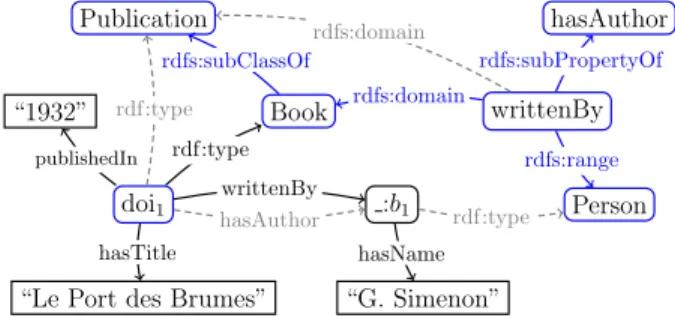
Example 2 (RDF graph with an RDFS ontology) Assume that the RDF graph G in the preced-ing example is extended with the RDFS on-tological constraints: (Book, ≺sc, Publication), (writtenBy, ≺sp, hasAuthor), (writtenBy, ←-d, Book) and (writtenBy, ,→r, Person). The resulting graph is depicted in Fig. 3. Its implicit triples are those represented by dashed-line edges.

RDF entailment. An important feature of RDF graphs are implicit triples. Crucially, these are con-sidered part of the RDF graph even though they are not explicitly present in it, e.g., the dashed-line G edges in Fig. 3, hence require attention for RDF graph summarization.

W3C names RDF entailment the mechanism through which, based on a set of explicit triples and some entailment rules, implicit RDF triples are de-rived. We denote by `iRDF immediate entailment,

doi1

Book Publication

“Le Port des Brumes”

:b1 “G. Simenon” “1932” Person writtenBy hasAuthor publishedIn rdfs:subClassOf rdfs:domain rdfs:range rdfs:subPropertyOf hasTitle writtenBy hasName rdf:type rdf:type hasAuthor rdf:type rdfs:domain

Figure 3: RDF graph and its implicit triples.

i.e., the process of deriving new triples through a sin-gle application of an entailment rule. More generally, a triple (s, p, o) is entailed by a graph G, denoted G `RDF (s, p, o), if and only if there is a sequence of

applications of immediate entailment rules that leads from G to (s, p, o) (where at each step, triples previ-ously entailed are also taken into account).

Saturation. The immediate entailment rules allow defining the finite saturation (a.k.a. closure) of an RDF graph G, which is the RDF graph G∞ defined as the fixed-point obtained by repeatedly applying `i

RDF rules on G.

The saturation of an RDF graph is unique (up to blank node renaming), and does not contain im-plicit triples (they have all been made exim-plicit by saturation). An obvious connection holds between the triples entailed by a graph G and its saturation: G `RDF (s, p, o) if and only if (s, p, o) ∈ G∞.

RDF entailment is part of the RDF standard itself; in particular, the answers to a query posed on G must take into account all triples in G∞[110], since in the presence of RDF Schema constraints, the semantics of an RDF graph is its saturation [107]. As a result, the summarization of an RDF graph should reflect its saturation, e.g., by summarizing the saturation of the graph instead of the graph itself.

Example 3 (RDF entailment and saturation) The saturation of the RDF graph comprising RDFS constraints G, displayed in Fig. 3, is the graph G∞ obtained by adding to G all its implicit triples that can be derived through RDF entailment, i.e., the

graph G in which the implicit/dashed edges are made explicit/solid ones.

We introduce below a few more notions we will need in order to describe existing RDF summariza-tion proposals.

Instance and schema graph. An RDF instance graph is made of assertions only (recall Fig. 2), while an RDF schema graph is made of constraints only (i.e., it is an ontology). Further, an RDF graph can be partitioned into its (disjoint) instance and schema subgraphs.

Properties and attributes of an RDF graph. While this is not part of the W3C standard, some authors use attribute to denote a property (other than those built in the RDF and RDFS standards, such as τ , ←-d etc.) of an RDF resource such that the property value is a literal. In these works, the term property is reserved for those RDF properties whose value is an URI.

Example 4 (Instance, schema, properties and attributes of an RDF graph) The RDF graph G shown in Fig. 3 consists of the

RDF schema graph comprising the blue triples, and of the RDF instance graph comprising the black triples. Further, within this G instance subgraph, the properties considered attributes are the following: publishedIn, hasTitle and hasName.

2.3

BGP queries

SPARQL3 is the standard W3C query langage used to query RDF graphs. We consider its popular con-junctive fragment consisting of Basic Graph Pattern (BGP) queries. Subject of several recent works [27, 95, 26, 78, 9], BGP queries are also the most widely used in real-world applications [78, 53]. A BGP is a generalization of an RDF graph in which variables may also appear as subject, property and object of triples.

3_{https://www.w3.org/TR/rdf-sparql-query/}

Notations. In the following we use the conjunctive query notation Q(¯x):- t1, . . . , tα, where {t1, . . . , tα} is a BGP. The head of Q is Q(¯x), and the body of Q is t1, . . . , tα. The query head variables ¯x are called distinguished variables, and are a subset of the vari-ables occurring in t1, . . . , tα; for boolean queries ¯x is empty. We denote by VarBl(Q) the set of variables and blank nodes occurring in the query Q. In the sequel, we will use x, y, z, etc. to denote variables in queries.

Query evaluation. Given a query Q(¯x):- t1, . . . , tαand an RDF graph G, the evaluation of Q against G is:

Q(G) = {Φ(¯x) | Φ : VarBl(Q) → Val(G) is a Q to G homomorphism such that {Φ(t1), . . . , Φ(tα)} ⊆ G}

where we denote by Φ(t) (resp. Φ(¯x)) the result of replacing every occurrence of a variable or blank node e ∈ VarBl(Q) in the triple t (resp. the distinguished variables ¯x), by the value Φ(e) ∈ Val(G).

Query answering. The evaluation of Q against G uses only G’s explicit triples, thus may lead to an incomplete answer set. The (complete) answer set of Q against G is obtained by the evaluation of Q against G∞, denoted by Q(G∞).

Example 5 (Query evaluation versus answering) The query below asks for the author’s name of “Le Port des Brumes”:

Q(x3):- (x1, hasAuthor, x2), (x2, hasName, x3) (x1, hasTitle, “Le Port des Brumes”)

Its answer against the explicit and implicit triples of our sample graph is: Q(G∞) = {h“G. Simenon”i}. Note that evaluating Q only against G leads to the empty answer, which is obviously incomplete.

2.4

OWL

Semantic graphs considered in the literature for sum-marization sometimes go beyond the expressiveness of RDF, which comes with the simple RDF Schema

ontology language. The standard by W3C for seman-tic graphs is the OWL [108, 109] family of dialects that builds on Description Logics (DLs) [4].

DLs are first-order logic languages that allow de-scribing a certain application domain by means of concepts, denoting sets of objects, and roles, denoting binary relations between concept instances. DL di-alects differ in the ontological constraints they allow expressing on complex concepts and roles, i.e., de-fined by DL formula. One of the most important is-sues in DLs is the trade-off between expressive power and computational complexity of reasoning with the constraints (consistency checking, query answering, etc.)

The first flavour of OWL [108] consists of three di-alects of increasing complexity: OWL-Lite, OWL-DL and OWL-Full. Unfortunately, very basic reasoning (concept satisfiability) in these dialects is highly in-tractable: ExpTime-complete in OWL-lite that cor-responds to the SHIFD DL, NExpTime-complete in OWL-DL that corresponds to the SHIOND DL, and even undecidable in OWL-full. A second flavour of OWL [109], a.k.a. OWL2, defines three new di-alects, OWL2 EL based on the E L DL, OWL2 QL based on the DL-liteR DL and OWL2 RL which can be expressed using logical rules. These new dialects comes with PTIME complexity for most of the rea-soning tasks. In particular, data management tasks (consistency checking, query answering, etc.) un-der OWL2 QL/DL-liteR ontologies have the same complexity as their counterparts in the relational database model [10].

3

RDF summarization: scope,

applications and dimensions

of analysis for this survey

As we shall see, RDF summarization has been at-tached many different meanings in the literature, and research is still ongoing. Therefore, we start with de-limiting the scope of RDF summarization as consid-ered in this survey (Section 3.1), before describing the RDF summary applications most frequently en-countered within this scope (Section 3.2), and finally

presenting several dimensions along which the cor-responding RDF summarization techniques can be classified (Section 3.3).

3.1

Scope

Our goal in this survey is to study summarization notions and tools which are useful to concrete RDF data management applications. We will thus dis-cuss a broad set of techniques, some of which are also used outside our target RDF data management contexts. However, to keep the survey focused, self-contained, and useful to RDF practitioners, we do not cover graph summarization or clustering techniques designed for very specific classes of graphs. For in-stance, while social network graphs can be modeled in RDF, such graphs have a very specific semantics, for instance, to reflect the important role of “user” nodes. Instead, we aim to cover summarization of general RDF graphs (without making assumptions on their application domain), without ontologies (in which case they basically coincide with labeled ori-ented graphs) or with ontologies (that are a specific, crucial feature of RDF data graphs).

Our review of the literature leads us to the follow-ing generic definition. An RDF summary is one or both among the following:

1. A compact information, extracted from the orig-inal RDF graph; intuitively, summarization is a way to extract meaning from data, while reduc-ing its size;

2. A graph, which some applications can exploit in-stead of the original RDF graph, to perform some tasks more efficiently; in this vision, a summary represents (or stands for) the graph in specific settings.

Clearly, these notions intersect, e.g., many graph summaries extracted from the RDF graphs are com-pact and can be used for instance to make some query optimization decisions; these fit into both categories. However, some RDF summaries are not graphs; some (graph or non-graph) summaries are not always very compact, yet they can be very useful etc.

3.2

Applications

We illustrate the above generic definition of an RDF summary through a (non-exhaustive) list of uses and applications.

Indexing. Most (RDF) summarization methods from the literature build summaries which are smaller graphs; each summary node represents several nodes of the original graph G. This smaller graph, then, serves as an index as follows. The identifiers of all the G nodes represented by each summary node v are as-sociated with the node v. To process a query on G, we firstly identify the summary nodes, which may match the query; then identify based on the index, the graph nodes corresponding to these summary nodes, as a first step toward answering the query.

Estimating the size of query results. Consider a summary defined as a set of statistics about prop-erty (edge label) co-occurrence in G, that is: the sum-mary stores, for any two properties a, b appearing in G, the number of nodes which have at least an outgo-ing a edge and at least an outgooutgo-ing b edge. If a query searches, e.g., for resources having both a “descrip-tion” and an “endorsement” in an RDF graph storing product information, if the summary indicates that there are no such resources, we can return an empty query answer without consulting G. Further, assume that a BGP query requires a resource with proper-ties p1, p2, somehow connected to another resource with properties p3, p4. If the summary shows that the former property combination is much rarer than the latter, a query optimizer can exploit this to start evaluating the query from the most selective condi-tions p1, p2.

Making BGPs more specific BGPs queries may comprise path expression with wildcards; these are hard to evaluate, as they require traversing a poten-tially large part of G. A graph summary may help understand, e.g., that a path specified as “any num-ber of a edges followed by one or more b edges” cor-responds to exactly two data paths in G, namely: a b edge; and an a edge followed by a b edge. These two

short and simple path queries are typically evaluated very efficiently.

Source selection One can detect based on a sum-mary whether a graph is likely to have a certain kind of information that the user is looking for, without actually consulting the graph. In a distributed query processing setting, this can be used to know which data partition(s) are helpful for a query; in a LOD cloud querying context, when answering queries over a large set of initially unknown data sources, this problem is typically referred to as source selection.

Graph visualization A graph-shaped summary may be used to support the users’ discovery and ex-ploration of an RDF graph, helping them get ac-quainted with the data and/or as a support for visual querying.

Vocabulary usage analysis RDF is often used as a mean to standardize the description of data from a certain application domain, e.g., life sciences, Web content metadata etc. A standardization commit-tee typically works to design a vocabulary (or set of standard data properties) and/or an ontology; appli-cation designers learn the vocabulary and ontology and describe their data based on them. A few years down the road, the standard designers are interested to know which properties and ontology features were used, and which were not; this can inform decisions about future versions of the standard4_.

Schema (or ontology) discovery When an on-tology is not present in an RDF graph, some works aim at extracting it from the graph. In this case, the summary is meant to be used as a schema, which is considered to have been missing from the initial data graph.

4_{Thanks to William van Voensel from schema.org for}

3.3

Classification of RDF

summariza-tion methods

From a scientific viewpoint, existing summarization proposals are most meaningfully classified according to the main algorithmic idea behind the summariza-tion method:

1. Structural methods are those which consider first and foremost the graph structure, respec-tively the paths and subgraphs one encounters in the RDF graph. Given the prominence of ap-plications and graph uses, where structural con-ditions are paramount, graph structure is promi-nently used in summarization techniques.

• Quotient: A particular natural concept when building summaries is that of quotient graphs (Definition 2). They allow charac-terizing some graph nodes as ”equivalent” in a certain way, and then summarizing a graph by assigning a representative to each class of equivalence of the nodes in the orig-inal graph. A particular feature of struc-tural quotient methods is that each graph node is represented by exactly one sum-mary node, given that one node can only belong to one equivalence class.

• Non-quotient: Other methods for struc-turally summarizing RDF graphs are based on other measures, such as centrality, to identify the most important nodes, and in-terconnect them in the summary. Such methods aim at building an overview of the graph, even if (unlike quotient summaries) some graph nodes may not be represented at all.

2. Pattern mining methods: These methods employ mining techniques for discovering pat-terns in the data; the summary is then built out of the patterns identified by mining.

3. Statistical methods: These methods summa-rize the contents of a graph quantitatively. The focus is on counting occurrences, such as count-ing class instances or buildcount-ing value histograms

per class, property and value type; other quanti-tative measures are frequency of usage of certain properties, vocabularies, average length of string literals etc. Statistical approaches may also ex-plore (typically small) graph patterns, but al-ways from a quantitative, frequency-based per-spective.

4. Hybrid methods: To this category belong works that combine structural, statistical and pattern-mining techniques.

Another interesting dimension of analysis is the required input by each summarization method, in terms of the actual dataset, and of other user inputs which some methods need:

1. Input parameters: Many works in the area require user parameters to be defined, e.g. user-specified equivalence relations, maximum sum-mary size, weights assigned to some graph ele-ments etc., whereas others are completely user independent. While parameterized methods are able to produce better results in specific sce-narios, they require some understanding of the methodology and as such limit their exploitation ability only to experts.

2. Input Dataset: Different works have different requirements from the dataset they get as in-put. RDF data graphs are most frequently ac-cepted, usually RDF/S and/or OWL are used for specifying graph semantics whereas only very few works consider DL models. In addition, some works consider or require only ontologies (semantic schema), whereas other works exploit only instances. Hybrid approaches exploit both instance and schema information. For instance, the instance and schema information can be used to compute the summary of the saturated graph, even if the instance graph is not saturated. For what concerns the summarization output, we identify the following dimensions:

1. Type: This dimension differentiates techniques according to the nature of the final result (sum-mary) that is produced. The summary is some-times a graph, while in other cases it may be just

a selection of frequent structures such as nodes, paths, rules or queries.

2. Nature: Along this dimension, we distinguish summaries which only output instance represen-tatives, from those that output some form of summary a posteriori schema, and from those that output both.

Availability: Last but not least, from a practical perspective it is interesting to know the availability of a given summarization service. This will allow a direct comparison with future similar tools:

1. System/Tool: Several summarization ap-proaches are made available by their authors as a tool or system shared with the public; in our sur-vey, we signal when this is the case. In addition, some of the summarization tools can be readily tested from an online deployment provided by the authors.

2. Open source: The implementation of some summarization methods is provided in open source by the authors, facilitating comparison and reuse.

We also consider the quality characteristics of each individual algorithm. Quality has to do with: com-pleteness in terms of coverage, precision and recall of the results if an “ideal” summary is available as a gold standard to compare with, the connectivity of the computed summary and, at the end, computa-tional complexity. Given variety of RDF summariza-tion approaches, it is not easy to define and evaluate a single meaningful notion of quality. A more com-prehensive, effort to establish a generic framework for computing quality metrics on summaries is proposed in [122], where authors discuss summarization qual-ity concerning both the schema and instances lev-els. However, difficulties remain, e.g. identifying the complexity of a summarization algorithm is not al-ways possible when the available description of the algorithm does not provide sufficient information.

The main categorization we retain for the dif-ferent RDF summarization approaches is based on their measurable/identifiable characteristics and not

on their intended use. This is because the bound-aries among the different usages are not very clear and there are types of methods that can be used in diverse cases/applications. Thus, the advantages and/or disadvantages for each category of methods cannot be identified in a generic way, however, we inserted a discussion whenever pertinent.

Fig. 4 depicts a high-level taxonomy of the RDF summarization works, based on the aforementioned dimensions. Note that many of the dimensions are orthogonal, thus a work may be classified in multi-ple categories. In the sequel, we classify the works, describe the main ideas and the implemented algo-rithms. Then we identify the specific dimension of analysis captured in Fig. 4 for each of these works.

4

Generic

graph

(non-RDF)

summarization approaches

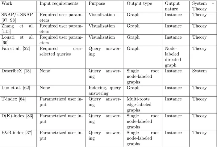
In this Section we review generic graph summariza-tion approaches. While these have not been specif-ically devised for RDF, they have either been ap-plied to RDF subsequently, or served as inspira-tion for similar RDF-specific proposals. An overview of the generic graph summarization works is pro-vided in Table 1 and Table 2. More precisely, Sec-tion 4.1 presents structural graph summarizaSec-tion methods, Section 4.2 describes works based on min-ing and statistics, while Section 4.3 considers sum-maries based on statistic and hybrid (structural and statistic) methods.

4.1

Structural graph summarization

The structural complexity and heterogeneity of graphs make query processing a challenging prob-lem, due to the fact that nodes which may be part of the result of a given query can be found anywhere in the input graph. To tame this complexity and di-rect query evaluation to the right subsets of the data, graph summaries have been proposed as a basis for indexing, by storing next to each summary node, the IDs of the original graph nodes summarized by this node; this set is typically called the extent. Given a query, evaluating the query on the summary and then

Figure 4: A taxonomy of the works in the area.

using the summary node extents allows obtaining the final query results.

4.1.1 Quotient graph summaries

Many proposals for indexing graph data are based on establishing some notion of equivalence among graph nodes, and storing the IDs of all nodes as the extent of the summary node. Formally, these correspond to quotient graphs, whose definition we recall below:

Definition 2 (Quotient graph) Let G = (V, E) be an A-edge labeled directed graph and ≡ ⊆ V × V be an equivalence relation over the nodes of V . The quotient graph of G using ≡, denoted G/≡, is an A edge-labeled directed graph having:

• a node uS for each set S of ≡-equivalent V nodes;

• an edge (vS1, l, vS2) iff there exists an E edge

(v1, l, v2) such that vS1 (resp. vS2) represents

the set of V nodes ≡-equivalent to v1 (resp. v2).

Prominent node equivalence relations used for graph summarization build on backward, forward, or backward-and-forward bisimulation [32]:

Definition 3 (Backward bisimulation) In an edge labeled directed graph, a relation ≈b between the graph nodes is a backward bisimulation if and only if for any u, v, u0, v0 ∈ V :

1. If v ≈b v0 and v has no incoming edge, then v0 has no incoming edge;

2. If v ≈b v0 and v0 has no incoming edge, then v has no incoming edge;

3. If v ≈b v0, then for any edge u−→ v there existsa an edge u0 a−→ v0 _{such that u ≈bu}0_;

4. If v ≈bv0, then for any edge u0 a−→ v0 _{there exists} an edge u−→ v such that such that u ≈ba u0. Forward bisimulation, noted ≈f, is defined sim-ilarly to backward simulation, but considers the out-going edges of v and v0, instead of the incoming ones. Forward and backward simulation, noted ≈f b, is both a backward and a forward bisimulation.

We already pointed out that, in Figure 1, the graph on the right is homomorphic to that on the left. The former is actually the quotient graph of the latter using ≈f b. In particular, the classes of ≈b-equivalent nodes are {1}, {2, 3, 4, 5}, {6, 8, 9}, {7}, those of ≈f -equivalent nodes are {1}, {2}, {3, 4}, {5, 6, 7, 8, 9},

and those of ≈f b-equivalent nodes are {1}, {2}, {3, 4}, {5}, {6}, {7}, {8, 9}.

Finally, we remark that it easily follows from the bisimulation definitions that if v ≈ v0, for instance for forward-bisimulation, then any label path that can be followed from v in the graph G can also be followed from v0 in G and the other way around. In other words, the same paths start (respectively, end) in two ≈-equivalent nodes. This condition is hard to meet in graphs that exhibit some structural heterogeneity: in such cases, every node is ≈-equivalent to very few (if any) other nodes.

The Template Index (or T-index) [64] summary considers that two graph nodes are equivalent if they are backward bisimilar. In particular, in a T-index, nodes represented together need to be reachable by the exact same set of incoming paths. The goal of the T-index is to speed up the evaluation of com-plex queries of a certain form (or template), such as P.v (all nodes v reachable by a path matching the regular expression P ) or v.P.u (all v, u node pairs connected by a path matching P ); the proposal gen-eralizes to arbitrary arity queries, although the au-thors note it is likely to be most useful in the above two simplest forms. The simulation relation between the nodes of a graph G is known to be computable in O(M ∗ log(M )) [71] or O(N ∗ M ) [32]; the cost drops to linear for acyclic graphs. All these algorithms as-sume the graph fits in memory.

To support efficient processing of graph queries that navigate both forward (in the direction of the graph edges) and backward, [37] describes the For-ward and BackFor-ward Index (F&B) which considers two nodes equivalent if they are undistinguishable by any navigation path composed only of forward and backward steps (see Figure 5 for an example). While this equivalence condition is very powerful, it is rarely satisfied by two nodes, thus the F&B index is likely to have a large amount of nodes (close to the number of nodes in the original graph), making the manip-ulation of the F&B index structure inefficient. To address the problem, the authors note that in prac-tice not any path query is frequently asked by appli-cations, therefore it suffices to consider F&B equiva-lence of nodes as being undistinguishable by forward and backward navigation along the paths from a

cer-tain set only.

Another method proposed in [38, 83], in order to make the F&B index smaller and more manageable, is to consider bisimilarity restricted only to paths of a certain length around the graph nodes (see Figure 5 for an example). This increases the chances that two nodes be considered equivalent, thus reducing the size of the bisimilarity-based summary. Limited bisimula-tion summaries like this, can be computed by evaluat-ing structural group-by queries (for k-bounded bisim-ilarity), respectively, queries derived from the work-load of interest (for workwork-load-driven F&B summa-rization). While the theoretical complexity of such queries is O(Mk_{), with M the number of edges and k} the size of the most complex query involved, efficient graph query processors, with the help of good index-ing, achieve much better performance in practice.

[18] considers the summarization of large Web doc-ument collections. While the main structure in this case consists of trees, they may also feature reference edges which turn the dataset into a global graph. The authors build a summary as a collection of regular ex-pression queries, such that the set of results to these queries, together, make up a partition over the set of nodes in all the documents of the input collec-tion. To each such regular expression is associated a set of cardinality statistics, to help application de-signers chose meaningful queries and inform them on the expected performance which may be reached on those queries. The dominant-cost operation required by this approach is computing simulations among N nodes; summaries can then be refined based on user-specified path queries.

[62] provides an I/O efficient external memory based algorithm for constructing the k-bisimulation summary of a disk-resident graph on a single ma-chine, based on several passes of sorting and grad-ually refining partitions of nodes on disk. The I/O complexity of the algorithm is O(k ∗ sort(Mp) + k ∗ scan(Np) + sort(Np)), where Mp, respectively, Np are the numbers of disk pages required to store the graph edges, respectively, graph nodes, while sort(·) and scan(·) quantify the cost of an external sort, re-spectively, the cost to scan a certain number of pages.

4.1.2 Non-quotient graph summaries

There are also many methods that construct non-quotient graph summaries. They distinguish nodes according to several criteria/measures and create summaries in which summary nodes represent multi-ple nodes out of the original graph.

A Dataguide [28] (see Figure 5 for an example) is a summary of a directed acyclic graph, having one node for each data path in the original graph. A graph node reachable by a set of paths belongs to the extents of all the respective Dataguide nodes. Thus, given a path query which may also contain wildcards, and a Dataguide, it is easy to identify the Dataguide nodes corresponding to the query, and from there their extents. The authors show how to integrate the Dataguide path index with more conventional in-dexes, e.g., a value index which gives access to all the nodes containing a certain constant value etc. A Dataguide is not a quotient: an input node may be represented by two Dataguide nodes, if it is reach-able by two distinct paths in the input graph. Build-ing a Dataguide out of a data graph amounts to de-terminizing an undeterministic finite automaton; the worst-case complexity of this is known to be expo-nential in the size of the input graph, yet only linear when the database is tree-structured.

Summary-based query answering with an accept-able level of error is considered in [41, 69]. The focus is on graph compression while preserving bounded-error query answering and/or the ability to fully re-construct the graph from the summary with the help of so-called “corrections” (i.e. edges to add to or re-move from the “expansion” of the summary into the regular part of the graph it derives from). The nodes of the resulting structural summary represent parti-tions of similar nodes from G, while a summary edge exists between two summary nodes u and v only if the nodes from G represented by u and v are densely connected. Similarly, [55] aims to compress G, but without considering corrections, while their edge la-bels represent the number of edges within each par-tition set, and the number of edges between every two such sets. To determine similar nodes, [41] re-lies on locality-sensitive hashing, while [69, 55] use a clustering method where pairs of nodes to merge are

chosen based on the optimal value of an objective function. In [84], the authors build on the concepts of [55] to show how to obtain in polynomial time, summaries which are close to the optimal one (in terms of corrections needed. However, these works focus on node connectivity, and ignore the node and edge labels which crucially encode the data content of an RDF graph.

[97] proposes the SNAP (Summarization on Grouping Nodes on Attributes and Pairwise Rela-tionships) technique, whose purpose is to construct, with some user input, a summary graph that can be used for visualization. A SNAP summary represents all the input graph nodes and edges: its nodes forms a partition of the input graph nodes, and there is an edge of type t between two summary nodes A and B if and only if some input graph node represented by A is connected through an edge of type t to an input graph node represented by B. Further, a SNAP summary has a minimal number of nodes such that (i) all in-put graph nodes represented by a summary node have same values for some user selected attributes and (ii) every input graph node represented by some sum-mary node is connected to some input graph nodes through edges of some user-selected types.

[22] considers reachability and graph pattern queries on labeled graphs, and builds answer-preserving summaries for such queries, that is: for a given graph G, summary S(G) and query Q, there exists a query Q0 which can be computed from Q, and a post-processing procedure P such that P (Q0(S(G))) = Q(G). In other words, eval-uating Q0 on the summary and then applying the post-processing P leads to the result Q(G). This property is rather strong, however, it is attained not under the usual query semantics based on graph homomorphism, underlying SPARQL, but under a bounded graph simulation one. Under these se-mantics, answering a query becomes P (instead of N P ), at the price of not preserving the query struc-ture (i.e., joins). The authors propose two paral-lel graph compression strategies, targeting different kinds of queries: (i) reachability queries, where we seek to know if one node is reachable from another; (ii) graph pattern queries, for which they attain a significant compression ratio. It should be again

Figure 5: Structural graph summarization examples.

stressed that the authors consider these queries under non-standard, more lenient semantics than the ones used for RDF querying. The complexity of build-ing their summaries are O(N ∗ M ) for reachability queries, and O(N ∗log(M )) for graph pattern queries.

4.2

Mining-based graph

summariza-tion

OLAP and data mining techniques applied to data graphs have considered them through global, aggre-gated views, looking for statistics and/or trends in the graph structure and content.

[112] leverages pattern mining techniques to build graph indices in order to help processing a graph query. It firstly applies a frequent pattern mining algorithm to identify all the frequent patterns with the size support constraint. Once the frequent pat-terns are extracted, they are organized in a prefix tree structure, where each pattern is associated with a list of ids of the graphs containing it. This prefix tree is then used to answer queries asking for the respective part of the graph. This approach by design does not reflect all data and is based on numeric information. [118] uses the same idea, but considers trees instead of graphs.

The Vocabulary-based summarization of Graphs

(VoG) [51] aims at summarizing a graph by its char-acteristic subgraphs of some fixed types, which have been observed encoding meaningful information in real graphs: cliques, bi-partite cores, stars, chains, and approximations thereof. VoG first decomposes the input graph, using any clustering method, into possibly overlapping subgraphs, the (approximate) type of each is then identified using the Minimum Description Length principle [85]. Finally, the input graph summary is composed of some non-redundant subgraphs, picked by some heuristic like top k, hence may not reflect all the input graph. Importantly, the VoG method has been shown to scale well; it is near-linear in the number of edges. The VoG code is avail-able for download5_.

An aggregation framework for OLAP operations on labeled graphs is introduced in [16]. The authors assume as available an OLAP-style set of dimensions with their hierarchies and measures; in particular, graph topological information is used as aggregation dimensions. Based on these, they define a “graph cube” and investigate efficient methods for comput-ing it. With a different perspective, [15] focuses on building out of node- and edge-labeled graphs, a set of randomized summaries, so that one can apply data

mining techniques on the summary set instead of the original graph. Using the summary set leads to bet-ter performance, while guaranteeing upper bounds on the information loss incurred.

A graph summarization approach, based solely on the graph structure is reported in [58]. It produces a summary graph that describes the underlying topol-ogy characteristics of the original one. Every sum-mary node, or super-node, comprises of a set of nodes from the original graph; every summary edge, or super-edge, represents an all-to-all connections be-tween the nodes in the corresponding super nodes. The goal of this work is to generate a summary that minimizes the false positives and negatives in-troduced by this summarization. The authors in-vestigate different distributed graph summarization methods, which proceed in an incremental fashion, gradually merging nodes into supernodes; the meth-ods differ in the way they chose the pairs of nodes to be merged, and cut different trade-offs between efficiency (running time) and effectiveness (keeping the false positives and negatives under control). The method termed Dist-LSH selects node pairs with a high probability to be merged; the probability is es-timated based on locality-sensitive hashing (LSH) of the nodes. The algorithms are implemented on top of the Apache Giraph framework.

[57] surveys many other quantitative, mining-oriented graph sampling and summarization meth-ods.

4.3

Statistical and hybrid graph

sum-marization

Several follow-ups on the SNAP summarization ap-proach (Section 4.1.2) have been proposed in the lit-erature.

The k-SNAP summarization approach [97, 98] is an approximation of the SNAP one. It allows setting the desired number k of summary nodes, so that a whole graph can be visualized at different granular-ity levels, similarly to roll-up and drill-down OLAP operations. A k-SNAP summary is a graph of k sum-mary nodes which satisfy the above condition (i) of a SNAP summary, but relax condition (ii) so that only some (not every) input graph node represented

by some summary node satisfies it. Further, as many such summaries may exist, a k-SNAP summary is defined as one that best satisfy the condition (ii) of SNAP summaries. Finding such a summary is NP-complete [97], hence tractable heuristic-based algo-rithms are proposed to compute approximations of k-SNAP summaries.

The k-SNAP summarization approach has been further extended [115] to handle numerical attributes, while k-SNAP as well as SNAP before have only con-sidered categorial attributes whose domains are made of a limited number of values. The proposed CANAL approach allows bucketizing the values of some nu-merical attribute into the desired number of cate-gories, hence reducing the summarization of graphs with categorial and numerical attributes to that of graphs with categorial attributes only. For a given numerical attribute a, each of the obtained categories represent a range of a values that nodes with similar edge structure have. Computing such categories is in O(N log N + k4

a), where ka is the number of dis-tinct a values that the input graph contains. Also, to ease the use of k-SNAP to inspect a graph in an roll-up and drill-down OLAP fashion, [115] provides a solution to automatically recommend k values for visualizing this graph. It consists in ranking k-SNAP summaries of varying k according to a so-called inter-estingness measure, defined in terms of conciseness, coverage and diversity criteria.

k-SNAP has also strongly inspired the summariza-tion approach in [60], which similarly aims at com-puting graph summaries w.r.t. user selected num-ber of summary nodes, attributes and edge types. The summaries are computed using a variant of one above-mentionned tractable k-SNAP heuristics, which keeps the SNAP condition (i) but changes the SNAP condition (ii) that k-SNAP tries to best sat-isfies, so that a summary best reflects the organiza-tion in social communities of the input graph nodes w.r.t. the selected attributes and edge types.

From a different perspective, [86] sketches SAP HANA’s approach for large graph analytics through summarization. It consists in defining rules to sum-marize part of an analyzed graph. Rules are made of two components, one graph pattern to be matched on the graph, and how the matched data should be

Work Input requirements Purpose Output type Output nature System -Theory SNAP/k-SNAP [97, 98]

Required user param-eters

Visualization Graph Instance Theory

Zhang et al. [115]

Required user param-eters

Visualization Graph Instance Theory

Louati et al. [60]

Required user param-eters

Visualization Graph Instance Theory

Fan et al. [22] Required user-selected queries Query answer-ing Graph Node-labeled directed graph Theory

DescribeX [18] None Query answer-ing

Single root node-labeled graphs

Instance System

Luo et al. [62] None Indexing, query answering

Graph Instance Theory

T-index [64] Parametrized user in-put Query answer-ing Multi-roots edge-labeled graphs Instance Theory

D(K)-index [83] Parametrized user in-put Query answer-ing Single root node-labeled graphs Instance Theory

F&B-index [37] Parametrized user in-put Query answer-ing Single root node-labeled graphs Instance Theory

Table 1: Graph summaries based on structural quotients.

grouped and aggregated into a result graph.

5

Structural RDF

summariza-tion

Structural summarization of RDF graphs aims at producing a summary graph, typically much smaller than the original graph, such that certain interesting properties of the original graph (connectivity, paths, certain graph patterns, frequent nodes etc.) are pre-served in the summary graph. Moreover, these prop-erties are taken into consideration to construct a sum-mary. The methods for structural summarization are distinguished into two categories. The quotient sum-marization methods, discussed in Section 5.1, while

the remaining structural summarization methods are described in 5.2

5.1

Structural

quotient

RDF

sum-maries

We begin with summarization techniques that are based on quotient methods. Intuitively, each sum-mary node corresponds to (represents) multiple nodes from the input graph, while an edge between two summary nodes represents the relationships between the nodes from the input graph, represented by the two adjacent summary nodes. Often, the nodes for-mulated in summaries like these, are called super-nodes, while their edges are called super-edges.

from the notion of quotient graph, relates query an-swers on an RDF graph G to query anan-swers on its quotient summary:

Definition 4 (Representativeness) Given an RDF query language (dialect) Q, an RDF graph G and a summary Sum of it, Sum is Q-representative of G if and only if for any query Q ∈ Q such that Q(G∞) 6= ∅, we have Q(Sum∞) 6= ∅.

Informally, representativeness guarantees that queries having answers on G should also have an-swers on the summary. This is desirable in order for the summary to help users formulate queries: the summary should reflect all graph patterns that occur in the data.

An overview of the structural quotient summaries is shown in Table 3. Section 5.1.1 introduces sum-maries defined based on bisimulation graph quotients (recall Definition 2), while Section 5.1.2 discusses other quotient summaries.

5.1.1 (Bi)simulation RDF summaries

The classical notion of bisimulation (Section 4.1) has been used to define many RDF structural quotient summaries.

Thus, [78] presents SAINT-DB, a native RDF man-agement system based on structural indexes. This index is an RDF quotient simulation, based on triple (not node) equivalence. The summary is not an RDF graph: its nodes group triples from the input, while edge labels indicate positions in which triples in ad-jacent nodes join. Thus, the index is tailored for re-ducing the query join effort, by pruning any dangling triples which do not participate in the join. Since the index contains only information on joins, and nothing of the values present in the input graph, the query language is restricted to BGPs comprising of vari-ables in all positions; further, these BGPs must be acyclic. For compactness, they bound the simula-tion, for small k values, e.g., 2; this enables com-pression factors of about 104_{. Semantic information} or ontologies are not considered. The time complex-ity of the algorithm comes from the corresonding al-gorithms for computing graph simulation. This is

O(N2∗ M ), where N is the number of nodes (equiv-alent types) and M is the number of edge labels in the result graph. In practice, different query process-ing strategies aimed at join prunprocess-ing are implemented by integrating the structural index with the RDF-3X [70] engine.

A structure-based index is proposed in [99], defined as a bisimulation quotient; the authors show that the summary is representative of only tree-shaped queries over non-type and non-schema triples, comprising a single distinguished variable which corresponds to the root node. Further, the authors study limited ver-sions of the bisimulation quotient by considering: (i) only forward bisimulation, (ii) only backward bisim-ulation or (iii) only neighborhoods of a certain length for tree structures of the input graph. The proposed applications of the structure index are twofold: (i) for data partitioning, by creating a table for each node of the structure index, thereby physically group-ing triples with subjects that share the same struc-ture, and (ii) for query answering, where the query may be run first on the structure index, to obtain the set of candidate answers, thus achieving prun-ing of the (larger) original graph. The authors do not consider graph semantics, nor answering queries over type and schema triples. The complexity of the corresponding algorithm for generating the index is O((N1∪ N2) ∗ M ∗ log N ), where N1 and N2 are the nodes selected for backward and forward bisimu-lation respectively, M is the number of edges and N the number of nodes of the input graph.

RDF summaries defined in [17] are quotients based on FW bisimulation. The authors do not consider graph semantics or ontologies. They show how to use the summary as a support for query evaluation: incoming navigational SPARQL queries are evaluated on the summary, then the results on the summary are transformed into results on the original graph by ex-ploring the extents of summary nodes. They propose in [45] an implementation based on GraphChi [52], the single-machine multi-core processing framework, to construct the summary in roughly the amount of time required to load the input KB plus write the summary. GraphChi supports the Bulk Synchronous Parallel (BSP) [106] iterative, node-centric process-ing model, by which nodes in the current iteration

execute an update function in parallel, depending on the values from the previous iteration. Their sum-marization approach is based on the parallel, hash-based approach of [6] which iteratively updates each node’s block identifier by computing a hash value from the node’s signature defined by the node’s neigh-bors from the previous iteration. The main idea is that two bisimilar nodes will have the same signa-ture, the same hash value, and thus have the same block identifier. Due to the large size of the result-ing bisimulation summary, the authors propose a so-called singleton optimization, which involves remov-ing summary nodes representremov-ing only one node from G; the reduced summary is therefore no longer a quo-tient of G.

ExpLOD [42, 43] produces summaries of RDF graphs, by first transforming the original RDF dataset into an unlabeled-edge-ExpLOD-graph, where a node is created for each triple in the orig-inal RDF graph, labeled with the triple property; unlabeled edges go from the original triple’s subject and object, to the newly constructed property node. Then, the ExpLOD graph is summarized by a forward bisimulation quotient, grouping together nodes having the same RDF usage. RDF usage can be statistical, e.g., the number of instances of a particular class, or the number of times a property is used to describe resources in the graph. RDF usage can also be structural, e.g., the set of classes to which an instance belongs, the sets of properties describing an instance, or sets of resources connected by the owl:sameAs property. As such, they do not propose one summary, but rather a framework where one can select the summary according to his ”usage” preferences. Finally, the bisimulation quotient is applied without taking into account neither schema nor type triples, thus the summary is not represen-tative. There are two sequential implementations of ExpLOD. The first implementation computes the relational coarsest partition of a graph using a partition refinement algorithm [72], and requires datasets to fit in main memory. The second ap-proach uses SPARQL queries against an RDF triple store; although in principle this is more scalable, as datasets need not be stored in main memory, it is slower due to the query answering time. To

Figure 6: RDF vocabulary for the data graph sum-mary [11].

overcome the limitation of the centralized approach, the authors extend ExpLOD, proposing a novel, scalable mechanism to generate usage summaries of billions of Linked Data triples based on a parallel Hadoop implementation [44].

[87] considers the problem of efficiently building quotient summaries of RDF graphs based on the FW bisimulation node equivalence relation. The authors do not reserve any special treatment to RDF type and schema triples, which prevents the resulting RDF summaries of being representative. Two implemen-tations of the algorithm for computing graph bisim-ulations, first introduced in [3], are presented: one for sequential single-machine execution using SQL, and the other for distributed execution, taking advan-tage of MapReduce parallelization to reduce running time. They both have worst-case time complexity of a O(M ∗ N + N2_).

5.1.2 Other structural quotient summaries To assist users whose task is query formulation, [11] creates the summary graph, the so called node collec-tion layer, by grouping nodes having the exact same types, or in the absence of types, the same outgo-ing properties, into entity nodes; further, nodes from the input with no outgoing properties, and having the same incoming properties from subjects with the same set of types, are represented by blank nodes. An edge exists between two summary nodes v1 and v2, labeled by a property p, if there exist two nodes v₁0 and v0₂ in G, such that v0₁ is represented by v1, v₂0 is represented by v2, and there exists an edge la-beled by p in G from v₁0 to v0₂. The number of

rep-resented nodes from the input is attached to each summary node, and the number of represented edges from the input to each summary edge. This summary graph may group resources from multiple datasets. The proposed dataset layer groups together nodes of the node collection layer which belong to the same dataset. Schema triples are not considered. The ap-proach bears similarities with ExpLOD, since nodes in the first layer are partitioned by types, and par-titions are represented by distinct summary nodes. However, unlike ExpLOD, the G nodes having a type, are not further distinguished by their data proper-ties, i.e., two nodes of the same type A, one having the data properties a, b and c and the other hav-ing the properties a and d will be represented by the same summary node. Unlike ExpLOD, their sum-mary graph is an RDF graph.

RDF summaries are defined in a rather restricted setting in [34]. The authors assume that all subjects and objects are typed, and that each has exactly one type; class and property URIs are not allowed in sub-ject and obsub-ject position, and no usage is made of possible schema triples. Under this hypothesis, they construct from the RDF graph a typed object graph (TOG) comprising (s, p, o) triples and assigning an RDF type for each such s and o. Two methods are proposed for summarizing the TOG, namely, equiva-lent compression and dependent compression. The equivalent compression produces a quotient of the TOG by grouping together nodes having the same type and the same set of labels on the edges adja-cent to the node. In the dependent compression, two nodes v1 and v2 of the TOG are grouped together if v1is adjacent only to v2, or vice-versa. As application scenarios of this approach the authors indicate min-ing semantic associations, usually defined as graph or path structures representing group relationships among several instances.

Based on query-preserving graph compression [22] (Section 4.1.2), an Adaptive Structural Summary for RDF graphs (ASSG, in short) is introduced in [114]. ASSG aims at building compressed summaries of the part of an RDF graph which is concerned by a cer-tain set of queries. The authors compute a structural rank of nodes, which is 0 for leaves, and grows with the shortest distance between the node and a leaf;

then, nodes having the same label and the same rank are considered equivalent, and are all compressed to-gether in a single ASSG node. To partition the N nodes of a graph G to different equivalent classes by their label and rank the cost is O(N + M ), where M the number of the edges of the graph.

RDF summaries defined in [13, 14, 12] adapt the idea of quotient summaries to two characteristic fea-tures of RDF graphs: (i) the presence of type triples (zero, one, or any number of types for a given re-source), and (ii) the presence of schema triples. As we explained in Section 2.1, RDF Schema informa-tion is also expressed by means of triples, which are part of G. [12] shows that quotient summarization of schema triples does more harm than good, as it de-stroys the semantics of the original graph. To address this, they introduce a notion of RDF node equiva-lence which ensures that class and property nodes (part of schema triples) are not equivalent to any other G nodes, and define a summary as the quotient of G through one such RDF node equivalence. Such summaries are shown to preserve the RDF Schema triples intact, and to enjoy representativeness (Defini-tion 4) for BGP queries having variables in all subject and object positions. The authors show how bisim-ulation summaries can be cast in this framework, and introduce four novel summaries based property cliques, which generalize property co-occurrence as follows. A clique cG is a set of data properties from G such that for any p1, p2∈ cG, a resource of G is the source and/or target of both p1and p2. For instance, if resource r1 has properties a and b while r2 has b and c, then a, b, c are part of the same source clique; if, instead, r1 and r2 are targets of these properties, then a, b, c are part of the same target clique. The so-called weak summary groups together nodes hav-ing the same source or target clique, while the strong summary requires the same source and the same tar-get clique; their variant typed-weak and typed-strong summaries first group nodes according to their types, and then according to their cliques. All these sum-maries can be computed in linear-time in the size of the input graph. A benefit of this specific approach is that clique summaries are orders of magnitude more compact than bisimulation summaries. The authors also study how to obtain the summary of G’s