A decision-making tool to maximize chances of meeting project commitments

HAL Id: hal-00746515

https://hal.archives-ouvertes.fr/hal-00746515

Submitted on 14 Sep 2013

HAL is a multi-disciplinary open access archive for the deposit and dissemination of sci-entific research documents, whether they are pub-lished or not. The documents may come from teaching and research institutions in France or abroad, or from public or private research centers.

L’archive ouverte pluridisciplinaire HAL, est destinée au dépôt et à la diffusion de documents scientifiques de niveau recherche, publiés ou non, émanant des établissements d’enseignement et de recherche français ou étrangers, des laboratoires publics ou privés.

A decision-making tool to maximize chances of meeting

project commitments

Nguyen Trong-Hung, François Marmier, Didier Gourc

To cite this version:

Nguyen Trong-Hung, François Marmier, Didier Gourc. A decision-making tool to maximize chances of meeting project commitments. International Journal of Production Economics, Elsevier, 2013, 142 (2), pp.214-224. �10.1016/j.ijpe.2010.11.023�. �hal-00746515�

A decision-making tool to maximize chances of meeting project commitments

Trong-Hung NGUYEN, François MARMIER*, Didier GOURC

UNIVERSITE DE TOULOUSE, MINES ALBI, CENTRE GENIE INDUSTRIEL ROUTE DE TEILLET, CAMPUS JARLARD, 81013 ALBI CEDEX 09, FRANCE

Abstract

The project management team has to respect contractual commitments, in terms of deadlines and budgets, that are often two antagonistic functions. Then, during the invitation to tender phase or when faced with a risk situation, it has to determine its risk management strategy. Based on the principles of a synchronized process between risk management and project management, we propose a decision-making tool to help the project manager choose the best risk treatment strategy.

The methodology developed, called ProRisk, uses the concepts of risk scenario, treatment scenario and project scenario to determine the consequences of possible risks combined or not with preventive and/or corrective treatment actions.

As a finding, the project manager is also able to indicate to the sales department if the financial and deadline conditions are sufficiently profitable with regard to the risks.

Keywords: decision support, project planning, risk management, scenarios, treatment strategy.

* Corresponding author. Tel: +33 563 493 312 (F. MARMIER)

1. Introduction

In the current context of market globalisation, and in order to find new clients, companies have to offer innovative products. They also have to change product ranges. More and more companies use project management tools and methods for managing their innovations, for ensuring better product quality, better deadlines and lower costs. In this context, particular attention is paid to project management methods by decision-makers and academics.

Every project type faces risks, whatever the size or topic concerned. Nevertheless, the more innovative the project, or if the technology area is poorly known, the more uncertain and risky the project. Professional organisations as well as standards bodies have for several years produced guides and books on project management and good practice (International Organization for Standardization (1997), IPMA (1999), Project Management Body of Knowledge or PMBoK, International Project Management Association Competence Baseline or ICB, etc.). These reference framework documents present the process required for management. Turner proposes a review of progress on the global project management body of knowledge (Turner 2000). He states that, even if the internal breakdowns may not be always appropriate, the guide to the PMBoK contains the core elements used by all project managers. The following dimensions are systematically mentioned in the reference framework documents: integration, scope, time, cost, quality, human resources, communication, risk and procurement management. Academic works also exist. These aim to reinforce their use (Themistocleous and Wearne 2000) and to add further details to the propositions in a range of different fields: defining and specifying notions of risk in order to reduce the polysemy of this term, they establish classifications and they propose new approaches.

In a project context, the manager has to take risks into consideration in two main situations. Firstly, when faced with a risk situation, the manager has to choose a strategy which keeps the project on budget and on time. Secondly, when the sales department answers an invitation to tender, risks have to be correctly evaluated and the strategies correctly chosen to obtain a realistic estimate (cost/duration) of the project.

This paper is interested specifically in approaches that allow projects to be managed by taking account of risks. These approaches aim to anticipate potential phenomena and to measure their possible consequences on the project life or objectives. They lead the manager to choose the risk treatment strategies appropriate to the project.

In the next part, we present a literature survey on risk management, which shows the diversity of the sectors of activity concerned. We illustrate the evaluation problematic of the influence of risk on project schedule. Then we describe our proposed methodology, “ProRisk”, and a case study is detailed. Finally, we analyse the results obtained and present our conclusions to this work.

2. The risk management approaches

The risk management area is large and concerns a huge number of activity sectors, from finance to industrial, via chemistry, nuclear technologies, health, the environment, etc. In several sectors, the need for methods has been known for a long time. Numerous approaches and methods have been developed and proposed as a result of directives and regulations

which are launched in the wake of more or less media-friendly disasters such as the Three Mile Island and Chernobyl nuclear accidents, the explosion at Bhopal, the floods at Vaison la Romaine, etc. Faced with these different disasters, populations have greater influence in their demands for more and more applications of the precaution principle. Then, to regulate the financial sector and promote corporate governance, several new regulations appear regularly, such as the Sarbanes-Oxley Act in USA or the financial security law in France.

2.1 Global approaches

In the literature, the risk management methods refer to a standard process presenting the well known steps: risk identification, risk evaluation and quantification, risk classification, proposed actions for treatment and/or impact minimization and risk monitoring (CSA 1997, BSI 2000, ISO 31000, PMI).

It would take too long to list every disaster and mention every method which has been proposed. Nevertheless, Tixier et al. propose a classification of 62 existing approaches (Tixier et al. 2002). They sort methods as being deterministic and/or probabilistic, but also qualitative or quantitative.

As an example of the deterministic and qualitative we can mention approaches that are dedicated to a particular activity, such as the HAZOP method (HAZard OPerability) for the chemical industry (Kennedy and Kirwan 1998), the HACCP method (Hazard Analysis Critical Control Point) for food chain security (Motarjemi and Käferstein 1999), or some more general ones that cover several activity sectors, such as PRA method (Preliminary Risk Analysis) (Nicolet-Monnier 1996).

For the probabilistic and quantitative approaches, there are the FTA method (Fault Tree Analysis) (Nicolet-Monnier 1996), the ETA (Event Tree Analysis) (Tiemessen and Van Zweeden 1998), the Monte Carlo method (Kalos and Whitlock 2008), or the two main approaches for project risk management: the RISKMAN method (Carter et al. 1996) and the PRAM method (Project Risk Analysis and Management) (Chapman and Ward 1997).

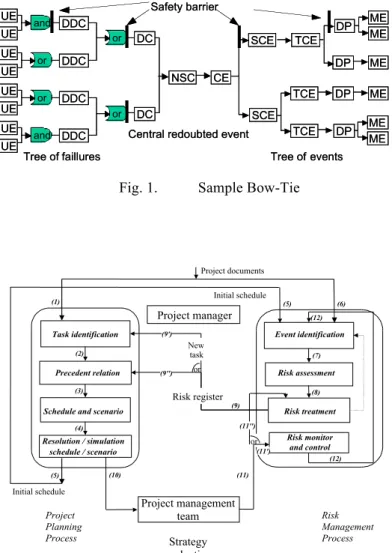
Deterministic and probabilistic and quantative such as the FMECA (Failure Modes, Effects and Criticality Analysis) (Rogers 2000), MOSAR or ARAMIS (Accidental Risk Analyse Methodology for IndustrieS) (Salvi and Debray 2006). The latter presents the bow-tie, which can also be helpful to manage risk in projects.

Deterministic and probabilistic and qualitative, such as the SRA method (Structural Reliability Analysis) (Rogers 2000). The approaches mentioned are summarized in Table 1.

[Insert Table 1 here]

In a project context corresponding to this work, a risk may introduce different modifications into a project. Tasks may appear or disappear, others could be longer or shorter than forecast. This therefore impacts the notion of project planning. The specificities of the project context are: the notion of uniqueness (there is no recurrence in the projects), the notion of limited horizon (there are different milestones and contractual commitments), and the notion of a multi-expertise environment (numerous actors with different skills, perceptions and points of view are working together); together, these influence the choice of method. Uniqueness leads

to use methods, such as the brainstorming, that are based on the expertise (very limited returns of experience and very few databases are available). The fact that time is limited forces the use of simple methods. Finally, the high number of actors implies that the model must share the information and help obtain a consensus.

In this work, we make the link between project planning, project management and risk management. To our knowledge, few methods are able to do that. They mainly apply risk management to an object, but the repercussions on planning are rarely modelled. Among the most closely-related approaches, RISKMAN examines the notion of risk as an event that can affect the project. PRAM mixes qualitative and quantitative elements by transforming events into uncertainties impacting the tasks (Chapman and Ward 2003), and the ARAMIS method allows the notion of the scenario to be highlighted. The risk becomes one or several uncertainties that are taken into account in tasks as a cost or delay range. It is reflected in the global project by the means of delay distribution or total project cost distribution. In the following part we provide more details concerning these three methods/methodologies that are, or that can be, used in the project risk area.

The RISKMAN method was developed between 1993 and 1996 during a EUREKA project (Carter et al. 1996). In accordance with existing reference framework documents, the RISKMAN methodology proposes a risk management process composed of the following phases: identification, evaluation, treatment and monitoring. The RISKMAN method recommends several interesting rules:

• a risk must always belong to only one risk category. 12 risk categories are proposed. The risks relate to: strategy, marketing, contracts, finance, project schedule, definition, process (Work Breakdown Structure or WBS), organisation (Organization Breakdown Structure or OBS), maintenance, business, and to external events outside organization;

• each impact has to be measured (or evaluated) within only one unit;

• a risk can have one or more causes. A risk can increase the probability of several others to appear (risk interdependence);

• each risk with no direct financial impact must lead directly, or indirectly, to one or more risks with a financial impact.

RISKMAN also proffers the notion of risk reduction strategy. A reduction strategy takes the form of an action required to reduce, eliminate or avoid the potential impact of a project risk. The scheduling of risk reduction must be applied at each project life-cycle phase, after the process of evaluating and quantifying the risks. In accordance with RISKMAN, the project manager can attenuate risk using different action types: avoidance, transfer, reduction, etc. Lastly, RISKMAN is a generic methodology applicable to all project types.

The PRAM method (Project Risk Analysis and Management) (Chapman and Ward 1997) was developed for the Project Managers Association. PRAM is supported by risk management process (RMP). This iterative process is composed by several steps such as define, focus, identify, structure, clarify, estimate, evaluate, plan or manage. The originality of this method comes from the simultaneous identification of the risks and of their associated reduction actions during the identification phase. Authors also indicate the case where reduction actions can generate new risks; therefore they talk about secondary risks.

The ARAMIS method comes from a European research project (2002-2004). The project objective was to develop a new evaluation methodology for risk evaluation responding to the

Seveso II European Directive requirements (Kirchsteiger et al. 1998). It was developed to be an alternative solution to deterministic or purely probabilistic approaches to risk evaluation. This methodology proposes the study of accident scenarios and the definition of protection barriers to halt the scenarios identified. ARAMIS uses results from other pre-existing methods, which already offered such dimensions, such as the MADS-MOSAR method. The representation of the accident scenarios using the bow-tie shape is at the heart of the ARAMIS methodology and represents one of its originalities. The risk is defined as a combination between the occurrence probability (frequency) of Dangerous Phenomena (DP) and their corresponding Major Events (ME), their intensity and the vulnerability of the territory exposed. The left side of the bow-tie, the fault tree, identifies the possible causes of a critical event. The combination of Undesirable Events (UE) leads to Detailed Direct Causes (DDC) and, when combined, to Direct Causes (DC). That generates the Necessary and Sufficient Conditions (NSC) inducing the Critical Event, then linking with Secondary Critical Events (SCE), Tertiary Critical Events (TCE), and then the Dangerous Phenomena. The bow-tie concept found in ARAMIS was initially developed by Shell to represent the different steps of risk management in an installation. On this basis, the ARAMIS authors present a particular version of the bow-tie, which combines a failures tree and an events tree (Fig. 1) (Salvi and Debray 2006). Protection Barriers can, therefore, be broken down into two families: preventive barriers, which are located on the bow-tie’s left side, and protection barriers which are on right (Fig. 1).

[Insert Fig. 1 here]

A possible way to move from left to right in a bow-tie, describes a scenario (cause – dreaded event - consequence). In each bow-tie, a dreaded critical event (CE) can result from several possible causes. Consequently, this tool is perfectly adapted to illustrate the result of a detailed risk analysis (such as FMECA, HAZOP).

2.2 Academic works

Several academic works propose methods to complement the different phases of the previously presented global approaches, such as optimisation of different criteria during the schedule or after the identification phase. As an example, Kiliç et al. propose an approach to solve a bi-objective optimisation problem where the makespan (or project duration) and the total cost have both to be minimized. Different preventive strategies are possible for each risk and a multi-objective genetic algorithm is used to generate a set of pareto optimal solutions (Kiliç et al. 2008).

Van de Vonder et al. are interested in generating robust projects by inserting buffers in the project schedule. Using heuristics, their approach aims to minimize project duration and maximize project robustness, which are antagonistic objectives. Depending on the project characteristics, this strategy can be an interesting way to increase solution stability (Van de Vonder et al. 2005).

In parallel to the previously presented global approaches, several authors propose methodologies to manage the risk in projects. Gourc et al. propose a reading grid of the risk management approaches following two families (Gourc 2006): the symptomatic approach and the analytic approach. The first approach group, called risk-uncertainty, is associated with

approaches where project risk management is transformed into project uncertainty management (Ward and Chapman 2003). This approach is supported by different software tools such as @Risk!, Pertmaster!, Crystal Ball!, etc. These software solutions use the Monte Carlo simulation method (Kalos and Whitlock 1970) to assess the duration, cost, etc., of a project in relation to the uncertainties. The second approach family considers risk as an event that can affect achievement of the project objectives (Carter et al. 1996). According to ISO/IEC Guide 73, “Risk can be defined as the combination of the probability of an event and its consequences” (ISO 2002). Software tools such as Riskman, RiskProject!, etc. continue this type of approach. The risk is described as an event, which has occurrence characteristics (potentiality to occur) and consequence characteristics on the project objectives (impact in the event of occurrence).

As observed in this literature review, little account is taken of risk and the strategies to deal with it regarding their repercussions on planning. The ability to present the project manager with a range of alternative risk treatments when faced with a risk situation, and the further ability to provide information on the consequences on decision criteria such as project cost and duration should improve the decision making process.

3. Risks consideration in project schedules

In this work, we propose to make the link between project management and risk management by analysing the consequences of a risk “as an event” (refer to the second approach family in section 2.2) in the project. This work is also complemented with the integration of risk treatment strategies that can be often translated as new project planning tasks. This leads the project manager to use a synchronised process between risk management and the project schedule process.

3.1 Limited analysis of the existing approaches

Project management and risk management processes are generally presented as independent. Each process is described with precision but the interrelations, which may exist, are never shown. This hypothesis is overly simplistic and leads to improper decisions. Pingaud and Gourc (Pingaud and Gourc 2003) propose a project management approach based on a synchronised process of project schedule and risk management, presented in Fig. 2.

[Insert Fig. 2 about here] This synchronized process illustrates:

• the initial scheduling influence of a project on the identification and evaluation of the project risks (steps (5) and (6) in Fig. 2);

• the influence of planned treatment actions to reduce the risk on a project schedule. The aims of the treatment actions are to either reduce the probability (from an initial probability to a reduced probability) and/or the impact (from an initial impact to a reduced impact). In this case, the authors refer to schedule with risk to indicate that the schedule takes into account the presence of risk in the project completion date evaluation and in the starting and completion date of each task (steps (9), (9’) and (9”) in Fig. 2). On the basis of these works, we propose here a tool designed to help managers to choose the strategy suited to the risks and contractual conditions.

This tool is mainly usable in two situations. First, faced with a known risk, it guides the project manager in the choice of a strategy that allows both budget and contractual deadline commitments to be respected. Secondly, when the sales department responds to an invitation to tender, the project manager can indicate if the proposed financial conditions and the defined deadline allow the different risks to be correctly integrated into the projected profitability and its realizability.

Therefore, the objectives of the proposed model are to:

• determine the impacts of the identified risks on the schedule (total execution duration, total cost, etc.). The traditional approach sorts risks separately in order to determine which risk is the most critical. The proposed approach allows determination of which risk sub-set (or scenario) is the most critical;

• determine the impacts of the treatment actions on the schedule (modification of the total duration, margin of each schedule task, reduction of the cost induced by unwanted events, modification of risk occurrence probabilities, etc.);

• help choose the best treatment strategy.

3.2 Illustration of the risks consideration in project scheduling

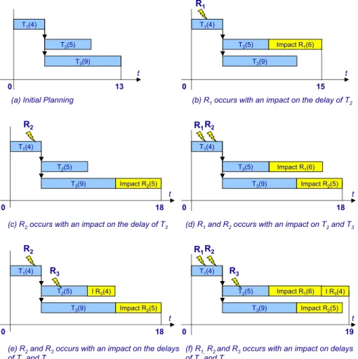
To illustrate the problematic, we propose a simple example comprising 3 tasks (T1, T2 and T3)

from a project initial schedule. 3 risks (R1, R2 and R3) have been identified. The initial impact

of each risk is illustrated in Fig. 3. Our objective is to correctly evaluate the influence of risk occurrences and to recommend treatment actions. Then we analyse each situation, (b) and (c) (Fig. 3) respectively, relative to the occurrence of risks R1 and R2. We notice a difference in the project completion date. Mover, in this example the project cost increases by 200 MU (Monetary Units) in (b) and 100 MU in (c). However, what about the situation where R1, R2 and R3 all occur?

Most risk management approaches studied separate each risk. Fan et al. propose a framework to choose a risk-handling strategy by looking at the project characteristics. The model provides a tool to understand the consequences and the financial implications of their decisions. For a given risk, their model takes into account delays and costs generated by the risk occurrence and occurrence probabilities through risk level (Fan et al. 2008). The objective is to decrease this level of risk but to be realistic about deadline and cost realities, the global impact of one or several risks is different from the total of each individual one. Therefore, situations (d) and (e) illustrate the occurrence impact of R1 and R2 or R2 and R3 on

the project deadline and, respectively, an increase of 300 MU and 150 MU. Situation (f) shows that in an additive way the effect of the occurrence of R1 and R3 modify the critical path and the total cost increases by 350 MU. Traditional approaches do not integrate the type of additive combination-only event that affects how tasks on the critical path would be evaluated.

[insert Fig. 3 about here]

Risk treatment actions can also have knock-on impacts on the schedule structure and the cost of the project. In such cases, treatment action implementation takes the form of:

• modifications in the WBS (Work Breakdown Structure). A treatment action can, for example, generate new tasks to achieve;

• modification of the tasks scheduling, since the precedence relation may be altered;

• extra costs due to new tasks. These can be a fixed cost or a proportional cost caused by the extended duration of pre-existing tasks.

Two treatment action types can be identified: preventive actions and corrective actions. Preventive actions aim to reduce the occurrence probability and/or the impact gravity by the mean of protection measures. These actions are notable for being undertaken before the risk occurrence. Therefore, they can be realized even if the phenomenon doesn’t occur. Corrective activities are performed to answer to the event occurrence. They reduce the impact importance.

Our objective is to propose a complete framework, taking account of all disturbances generated by a risk. It should permit evaluation of its consequences on project management, particularly on the deadline dimension. In addition, this environment will be useful for managers, in order to measure the project global risk level, by taking into account the different possible scenarios, as well as helping to choose the most suitable risk strategies.

4. Proposed model

Taking decisions in the choice of a risk treatment strategy for a project is a multicriteria problem. However when the project manager has to take the decision, the number of criteria used to measure the impact of the proposal is most often reduced to the main ones: the probability of the scenario, the cost, which is a sensitive and finite resource, and the delay, which is traditional a matter of contractual commitment.

4.1 Hypothesis

The proposed model is based on 2 main hypothesis. First, the risk integration to the project management is done regarding the deadlines and the cost criteria. The considered impacts (modification or suppression of an existing task or the insertion a new task for example) influence on the project total duration and cost. The resource aspects such as availability or skill are not considered for the moment in the model.

Another hypothesis used for this model is that, at the beginning of the project, the tasks list and the risks list are known and do not vary during the project. Every characteristic relative to the risks are known since an approach such as the Delphi method has been previously applied (Dalkey and Helmer 1963). This method helps risks manager characterizing the risk dimension (impact and probability). It uses different anonymous questionnaires for eliciting experts’ opinion to reach a consensus. The risk assessment step can require gathering a huge number of data. This work hasn’t for objective to develop a tool making easier the data-gathering that may be costly in time and effort with a realistic number of tasks.

When new risks are identified and quantified during the project, these can be integrated into the risk scenarios calculation, allowing the approach to retain a large degree of reactivity and realism. The uncertainties are not managed in this work. Therefore, it is possible to apply the model at the project by starting to analyse the project global risk level, the possible scenarios and the selection of the best treatment strategies. Later, during the project, the same questions can be solved by a risk scenario analysis of risks already run on the completed tasks.

4.2 Data

A project is described by its tasks Tt (t=1…T), T being the number of project tasks. The planning process gives an initial planning Pi that doesn’t integrate any risks. A project is also described by its set ER of identified risks Ri (i=0…n), n being the number identified risks. Each Ri is characterised via the risks management process. It has a probability and an impact. The initial impact allows consideration of the fact that the task is running in a graceful degradation. A risk Ri is also characterized by its period of occurrence, i.e. the tasks during

which the risk can occur.

A risk scenario ScRs corresponds to a combination of the risks that are considered as occurring. A project presenting n risks leads to 2n risks scenarios. Then ScRs (s=1…2n) is a possible achievement with k risks ( 0! k ! n) and the total number of risk scenarios,

presenting k of the n identified risks, is equal to

n! k !(n ! k)!.

Each risk can be treated in various ways that can be preventive, corrective or a combination of several actions. A risk Ri can be associated to one or more treatment strategies StTij (j=1…m), m being the number of identified strategies for Ri. A treatment strategy StTij groups a set of treatment actions Aij! (!=1…a) to avoid or reduce the risk Ri, a being the number of identified

treatment actions. A treatment action can be materialized by a task to achieve and it can introduce 3 types of modification to the WBS:

• addition of a new task, which generates a new action to realize;

• suppression of a task from the initial schedule. The risk is reduced by suppressing a task from the schedule;

• modification of an existing task that can be resumed by the suppression of a task and the addition of another one.

A treatment strategy is a preventive strategy if it contains at least a preventive treatment action. Otherwise, it is a corrective strategy. If the strategy consists in running no action at all, it is noted as being an empty set such as ".

Finally, for each risk Ri several treatment strategies are possible. The definition of these strategies can lead to the appearance of treatment actions common to several risks. The set of all the identified StTij for a risk Ri is written StRi.

Then StR_i = !,

{

}

Card (StRi) = m + 1

A treatment scenario ScTd (d=1…D) corresponds to a combination of the treatment strategies chosen to deal with the different risks of a project. The set of treatment scenarios is given by:

E ScT = StRi i =1 n

!

The probability and the impacts (delay and cost) are qualified of initial before the development of the risk management approach. They are qualified of reduced if they are modified after the achievement of the treatment actions.

Then, a project scenario ScPp (p=1…P) is defined as being a possible project achievement that is built with a risk scenario and treatment scenario (ScPp=<Pi, ScRs, ScTd>). The set of project scenarios ES is obtained by combining the set of occurring risks (or a risk scenario) and the set of determined treatment actions (or treatment scenario).

4.3 Proposed new resolution approach: ProRisk

To evaluate the different possible project scenarios, the management team need to generate an initial schedule, without integrating the notions of risk and treatment. It then needs to calculate the different risk and treatment scenarios. These scenarios allow the set of the project scenarios to be constructed. Finally, when the project scenarios are known it is possible to obtain their durations and their costs. Therefore, the proposed method uses data from the schedule process (management team) and from the risk management process; as presented in Fig. 4, ProRisk contains six modules:

• Initial schedule generation.

The initial schedule generation allows the project schedule to be created by considering the whole project tasks, their precedence links and initial duration. The duration obtained is the total project duration that corresponds to the schedule, without taking into account the risks.

• Risk scenarios generation.

The module is the list of the different risks. The objective of the risk scenarios generation is to generate all possible risk sub-sets.

• Treatment scenarios generation.

The different possible treatment strategies and the actions they contain to deal with each risk and their effects are introduced in this module. Treatment scenario generation consists in determining all possible treatment scenarios.

• Project scenarios construction.

This module takes the different risks and project scenarios to generate the whole project scenario.

The first iteration of the project scenario construction function lists possible scenarios with only one risk (R1 for example).

ES1= !; R₁;( R₁, StT₁₁)

{

}

{

}

The notation (_,StT11) indicates the fact that the treatment strategy (preventive) is done and avoids the achievement of risk R1.

The second iteration allows constructing a scenario by adding a second risk (R2 for example). For example, if StT11 and StT21 are corrective strategies respectively for risks R1 and R2, then:

ES 2= !; R₁;( R₁, StT₁₁); R₂; R₁R 2;( R1, StT11)R2; ( R₂, StT₂₁); R₁( R₂, StT₂₁);( R₁, StT₁₁)( R₂, StT₂₁) " # $ %$ & ' $ ($ …

Finally, we obtain the possible scenario total set by considering all the possible risks combinations.

ESn= ScP

{

}

{

}

However, some obtained scenarios can present the following inconsistency:

For 2 different existing risks Rx and Ry, belonging to a same ScRw (Rx"ScRw and Ry"ScRw).

ScTz presents two treatment strategies StTxk and StTyl containing respectively the following treatment actions Axk1 and Ayl1. With:

Axk1: suppressed T2 Ayl1: replaced T2 by T5

All project scenario ScP presenting a treatment scenario including both actions Axk1 and Ayl1 is inconsistent and is eliminated.

• Probability calculation of each project scenario.

The probability calculation method for each project scenario differs due to the fact that the project scenarios contain, or do not contain, a treatment strategy. It is not an objective of this module to determine whether a risk exists or not, or to evaluate its characteristics. However, during a project, using data relative to newly identified and quantified risks, the proposed approach permits progressive completion/modification of the set of project scenarios using the newly acquired knowledge.

If the scenario does not contain any treatment strategy, the calculation is applied on the initial occurrence probabilities of the risks comprising the risk scenario.

proba < ScR

(

)

( )

(

)

( )

(

)

(

With proba(Ri) the probability that the event related to Ri occurs. This probability is also called initial probability.

If ScP contains a ScT, four possible situations allow the probability to be determined.

proba < ScR

(

)

'

proba(Ri StTij) is the probability that the event related to Ri occurs knowing that StTij

has been done. This probability is called reduced probability. Then, for each risk it uses either reduced probabilities, where the risk treatment strategy is preventive, or the initial probability where the strategy is corrective.

(1) if (R_i!ScRs) and

(

(

)

(

( )

(

)

)

)

In this first case, the event relative to Ri occurs and there is no strategy launched, or the

(2) if (R_i!_ScR

s) and

(

(

)

(

( )

(

)

)

)

Either Ri is not occurring or a preventive strategy that does not modify the probability has

been used.

(3) if (R_i!_ScR

s) and (StTij is preventive) and proba R

(

( )

(

)

)

In this ScP, Ri is occurring. It is influenced by the preventive strategy and the initial

probability of Ri is modified.

(4) if (Ri !_ScR

s) and (StTij is preventive) and proba R

(

( )

(

)

)

A preventive strategy has been processed and the initial probability has been modified. Finally Ri is not occurring.

• Duration and cost calculation of each project scenario.

For each project scenario, the duration and the cost are calculated by taking into account potential modifications induced at the schedule level by the achievement of treatment strategies. The PERT method is used to calculate the project scenario duration. After having adapted the initial schedule in accordance with the studied scenario (modified duration, tasks added or removed), the project scenario duration is computed by taking into account the earliest starting dates.

The cost of a project scenario without taking into account risks C

R

(

)

only cost of the T tasks that constitute the initial project planning. With !p,C

R

(

)

( )

T

"

The initial cost of a project scenario ScP_p =< Pi,ScRs,!>is determined as being:

C_Rinitial _ScP p

(

)

( )

"

{

}

Where GCiinitial corresponds to the Global Cost of Ri induced by the cost impact CIi of Ri that is the fixed part of the total cost (materials, tools, parts, etc.) and by an indirect cost that depends on the action duration, through the Delay Impact DIi, and on the actors through the rate Vt of the resource in charge of task t.

GCinitial R i

( )

!

!

(

)

"

Finally, the cost of a project scenario including a treatment scenario ScP_{p =< Pi,ScRs},ScT_{d >}

C ScP

(

)

( )

"

"

"

{

}

With the reduced global cost impact (GCreduit R

i

( )

GCreduced R i

( )

!

!

The cost of a treatment strategy StTij is determined by:

C(StT_ij) = C( A_ij!)

! =1

a

"

{

}

{

}

Where the cost of the action is composed by a direct cost C

ij!

direct

that is the fixed part of the total cost (materials, tools, etc.) and by an indirect cost C

ij!

indirect

that depends on the action duration and on the actors.

C( Aij!) = Cij! direct +C ij! indirect ,"i # 1...n

{

}

{

}

{

}

[insert Fig. 4 about here]

This methodology and tool are flexible. That makes possible to obtain statistics before the project launching, as well as during the project lifecycle, by taking into account the current date and the state of the different risks and tasks.

5. Case study

To validate our proposals, we take as an example a condensed case, extracted from a study that we carried out previously. This study examines the case of a building project for a weather-forecasting station. Different actors from different sectors take part in the project. The different data have been collected from the different project participants, particularly the project manager. At the end of the case study, results are discussed with the project manager and the solutions deduced using ProRisk are compared in the light of their effectiveness.

5.1 Presentation

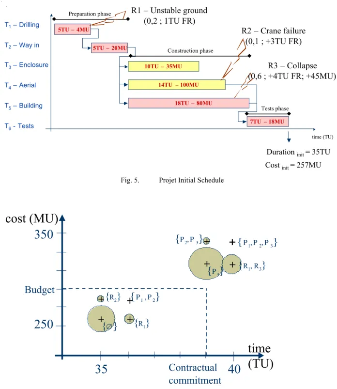
The project comprises 3 main phases, each comprising 6 tasks (T1 to T6), presented in Fig. 5.

[insert Fig. 5 about here]

3 risks are identified by the risk management process (R1 to R3). Therefore, in this project,

EScR (the set of the risk scenario) contains 23 risk scenarios:

Each risk is characterised by a probability, a period of occurrence, an initial impact (cost and duration) and associated treatment strategies (i.e. Table 22).

[insert Table 2 about here]

Each treatment strategy, as detailed in Table 3, presents a duration, an insertion location in the logical network or a task to be modified, a cost, a reduced probability and reduced impact (reduced cost and reduced duration) of the treated risk.

[insert Table 33 about here] 5.2 Results

The first results obtained, presented in Table 4, are the project scenarios without any treatment strategies. Scenarios can be sorted by occurrence probabilities, deadlines, costs, or criticity criterion, combining the cost and deadline dimensions. In Table 4, scenarios are sorted by their criticity in descending order.

[insert Table 4 about here]

Table 5 presents the results obtained by running the different project scenarios. All the combinations of risk scenario and treatment scenario are tried and then, each project scenario is different from the others. In Table 5, scenarios are sorted by their criticity.

[insert Table 5 about here]

The scenario durations in Table 4 and Table 5 are presented by time unit (TU) and achievement cost in monetary unit (MU).

To choose the appropriate treatment strategy, which is a multi-criteria decision problem (duration and cost), an aggregated criterion representing a global impact is proposed. In order to make the criteria comparable we introduce, for each project scenario, # and $ respectively represent the duration and the cost metrics:

! = d max(d ) and ! = c max(c) Then, !," # 0,1$% &'

Where d is the duration of a given project and c its cost, max(d) is the duration of the longest project scenario and respectively max(c) the cost of the most expensive project scenario. Then, the global impact is obtained using the following formulae:

impact = p ! " + q ! #

Where p and q are two coefficients that are chosen by the project manager in accordance with the importance criterion. In this study, we considered the weight of each criterion (cost and duration) as equivalent for the calculation of the criticity. Then p=q=0.5. However, project

manager preferences can be different and lead to variation in criticity and therefore to a different risk scenario hierarchy.

Criticity (Cr) is then obtained as follows, using the global impact of the scenario and its probability (P):

Cr=P x impact 5.3 Analysis

5.3.1 General observations

Through Table 4, it can be seen that the most probable risk scenario, which is the scenario presenting at least one outcome risk, is the one containing R3: {R3}. Logically, scenarios

containing R2 (P(R2)=0,1) are the least probable. Globally, through Table 4, the cheapest

solution corresponds to the project scenario in which no risk occurs: {"}. This solution is also the quickest with the one presenting {R1} that may occur during a task which is not

located on the critical path. The most expensive scenario is the one presenting {R1, R2, R3}

and therefore these consequences lead to the longest scenario. Because of the very low probability, even if 3 risks occur, the scenario where {R1, R2, R3} occurs is not the most

critical one. But it is also not the least probable, which is the one containing (R1 and R2).

Preventive treatment strategies aim to decrease the risk criticity by acting on the risks probability and/or their impacts. If we consider possible treatment scenario, Table 5 presents the modifications generated by these strategies on the probabilities, on the impacts or on the criticity. Then, Table 55 presents a different classification from Table 4.

In the proposed case study, if we consider a risk scenario {R2}, it is possible to apply StT21.

StT21 modifies the R2 impacts. In fact, R2 has no impact on deadlines, only on costs. StT21

leads to reductions in R2 cost impact, but involves an additional duration. This shows that

strategies require attention because they can lead to modifications in the project duration. But project manager want to be sure that they will be able to lead the project by meeting the budget and the stated deadline. One means is to avoid risks using preventive strategies. This leads managers to ask the question: “which strategy to choose if we want to maximize the probability of the scenario where no risk occurs?” In the case study, if we want to maximize this probability, the strategy StT33 should be adopted. Without any strategy, the probability

that no risk occurs is P({"})=0.288, and with StT33 the probability becomes P({_, StT33

})=0.677. This is explained by the fact that P({R3}) is decreased from 0.432 to P({R3, StT33

})=0.043. This risk scenario ({R3}) is also the most critical risk scenario, StT33 allows a

decrease in criticity in case of R3 occurring.

5.3.2 About taking decisions

For project managers there are two situations can require analysis and where such support would be helpful. First, if the manager is in the project conception phase, s/he has to provide target costs and deadlines. Knowing the different risks, s/he has to estimate the chances of success, as well as of meeting the budget and the contractual commitments. Fig. 6 presents the different risk scenarios with the project duration in x-coordinate and its cost in y-coordinate.

The probability of the scenario is represented by the bubble diameter. Therefore, an acceptability zone can be defined Fig. 6, using the budget and deadline thresholds.

[insert Fig. 6 about here]

Fig. 6 makes is possible to see and understand the problematic relating to the different risk scenarios presented in Table 4. The risk scenarios {R1} and {R2} stay within the required

budget and deadline. However {R3}, or the risk scenarios combining R3 and R1 and/or R2,

exceed the acceptability zone presented in Fig. 6. Moreover, {R3} presents a high probability

level compared to other risk scenarios. Therefore, the project manager will concentrate her/his efforts, and suggest risk treatment strategies, for R3.

Secondly, if the project manager considers (or faces) a particular risk scenario, s/he has to analyse the improvements obtained with the different possible strategies. S/he then has to choose the most appropriate treatment scenario for a given risk scenario. The question is, for any given risk scenario, which risk strategy is the most appropriate?

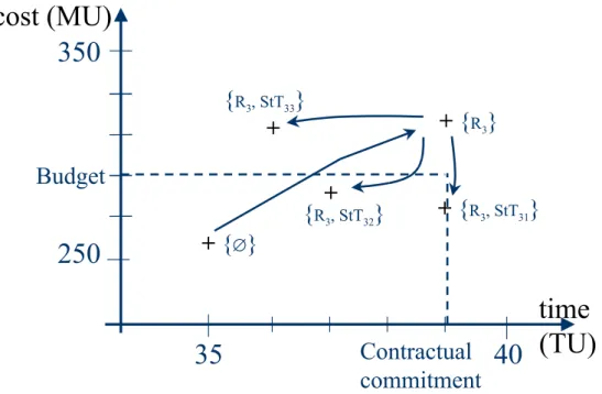
In the case study presented here, three strategies are possible for the risk scenario {R3}. Fig. 7

presents the possible treatment strategies. However, if R3 occurs, only {StT31} and {StT32}

will meet the budgetary and contractual requirements. As risk scenario{R3} presents a

relatively high probability level, it may be sensible to apply one of these two strategies. The results obtained and the choices suggested were compared and discussed according to the project actors’ perceptions. The treatment strategy proposed by ProRisk does indeed correspond to that which the decision maker would have selected and applied.

[insert Fig. 7 about here]

Then, the project manager is able to deduce whether the project is profitable, taking into account the associated probability. One possible conclusion is that the negotiation conditions are not acceptable because the probability of being in the acceptability zone at the end of the project is too low. Therefore, s/he can indicate to the sales department that the contract conditions have to be reviewed.

Finally, it is also possible to observe that risk scenarios combining several risks such as {R1,

R3} for example, are more critical and also more probable than some risk scenarios presenting

only one risk. This example validates the relevance of studying the scenario, contrary to the traditional approach that considers risks on a separate basis.

6. Conclusion and Perspectives

To estimate the risk level for each project, in this paper we propose an approach that makes it possible to model and evaluate the impact of risks on the project cost and the schedule cost. This approach uses the synchronized processes principle. Then, we defined the concepts of risk scenario, treatment scenario and project scenario. The principles of the proposed ProRisk method have been illustrated in a case study.

The ProRisk methodology is well suited to promote and favour exchanges between project scheduling teams and risk management teams. It can be used from the project conception phases to assist with project launch decision. It allows an estimate to be made of the global

risk level and gives a vision of the possible scenarios: from the least to the most probable, from the most disastrous to the most optimistic!

It is also usable during the project life-cycle, to estimate a project scenario that may occur knowing the risks that have already occurred. Moreover, we show that in several situations the traditional risk hierarchies, obtained through traditional approaches, lead to hierarchisations that are not relevant. The fact is that considering risk scenarios instead of single risks gives results that are closer to the reality. A software tool has been developed (java platform), it implements the functionalities described in this paper.

During a project, risk sources can be the cause of other risks (Carter et al. 1996) and the risk impacts can change the environment for other risks. However, we observe that all the different project risk analysis methods study risks under the hypothesis of independence between risks. These risk behaviours are individually easier to identify and easier to generate. However, in reality interdependencies exist between risks. These interdependencies can be strong enough to change the parameters of certain risks, such as the probability and/or the impact if one or more risks occur simultaneously. Even if in some cases a risk may be another risk factor (Carr and Tah 2001), it also has to be used to calculate other risk parameters. As a result, the risk impact evaluation can be influenced by these interdependencies. The influence mechanisms are currently implemented. The main perspective for this work will be to examine the influence of previously-occurring risks on the probability scenarios. It consists in using a model to take account of the interdependency mechanisms, or influences between risks. Therefore, different rules can be imagined based on the occurrence/ non-occurrence of risks that may have an impact on other risks characteristics, but that also may involve the occurrence/ non-occurrence of others risks.

7. References

British Standards Institution, 2000. BS 6079-3: Project Management: Guide to the management of business related project related.

Canadian Standard Association, 1997. CAN/CSA-Q850: Risk Management, Guideline for Decision Makers.

Carr, V. and Tah, J.H.M., 2001. A fuzzy approach to construction project risk assessment and analysis: construction project risk management system. Advances in Engineering Software, 32(10-11), 847-857.

Carter, B., Hancock, T., Morin, J. and Robin, N., 1996. Introducing RISKMAN: the European project risk management methodology, The Stationery Office.

Chapman, C.B. and Ward, S.C., 1997. Project risk management: processes, techniques, and insights, John Wiley and Sons.

Dalkey, N. and Helmer, O., 1963. An Experimental Application of the Delphi Method to the Use of Experts, Management Science, 9(3), 458-467.

Fan, M., Lin, N. and Sheu, C., 2008. Choosing a project risk-handling strategy: An analytical model. International Journal of Production Economics, 112(2), 700-713.

Gourc, D., 2006. Towards a general risk model for piloting goods- and service-related activites (Vers un modèle general du risqué pour le pilotage et la conduite des activités de biens et de services). HDR de l’Institut National Polytechnique de Toulouse, France.

International Organization for Standardization, 1997. ISO 10006, Quality Management. Guidelines to Quality in Project Management.

International Organization for Standardization, 2009. ISO 31000, Risk management -- Principles and guidelines.

International Organization for Standardization, 2002. ISO Guide 73, Risk management -- Vocabulary -- Guidelines for use in standards.

International Project Management Association, 1999. IPMA Competence Baseline. http://www.ipma.ch.

Kalos, M.H. and Whitlock, P.A., 2008. Monte Carlo methods, Wiley-VCH.

Kalos, M.H. and Whitlock, P.A., 1970. Monte Carlo Methods. Computers and Their Role in the Physical Sciences.

Kennedy R., Kirwan B., 1998. Development of a Hazard and Operability-based method for identifying safety management vulnerabilities in high risk systems. Safety Science, 30(3), 249-274.

Kiliç, M., Ulusoy, G. and Serifoglu, F.S., 2008. A bi-objective genetic algorithm approach to risk mitigation in project scheduling. International Journal of Production Economics, 112(1), 202-216.

Kirchsteiger, C., Christou, M. and Papadakis, G., 1998. Risk Assessment & Risk Management in the Context of the Seveso II Directive, Elsevier, The Netherlands. Motarjemi, Y. and Käferstein, F., 1999. Food safety, Hazard Analysis and Critical Control

Point and the increase in foodborne diseases: a paradox? Food Control, 10(4-5), 325– 333.

Nicolet-Monnier, M., 1996. Integrated regional risk assessment: The situation in Switzerland. International Journal of Environment and Pollution, 6(4-6), 440–461.

Pingaud, H. and Gourc, D., 2003. Approach of controlling an industrial project by the risk analysis (Démarche de pilotage d’un projet industriel par l’analyse des risques). 5e Congrès International Franco-Québécois de Génie Industriel, Canada.

Rogers, R.L., 2000. The RASE Project risk assessment of unit operations and equipment, http//www.safetynet.de/EC-Project, pp1-50.

Salvi, O. and Debray, B., 2006. A global view on ARAMIS, a risk assessment methodology for industries in the framework of the SEVESO II directive. Journal of Hazardous Materials, 130(3), 187-199.

Themistocleous, G. and Wearne, S.H., 2000. Project management topic coverage in journals. International Journal of Project Management, 18(1), 7-11.

Tiemessen, G. and Van Zweeden, J.P., 1998. Risk assessment of the transport of hazardous materials. In Proceeding from ninth international symposium loss prevention and safety promotion in the process industries. pp. 299–307.

Tixier J., Dusserre G., Salvi O. and Gaston D., 2002. Review of 62 risk analysis methodologies of industrial plants, Journal of Loss Prevention in the Process Industries, 15(4), 291-303.

Turner, J.R., 2000. The global body of knowledge, and its coverage by the referees and members of the international editorial board of this journal. International Journal of Project Management, 18(1), 1-5.

Van de Vonder, S., Demeulemeester, E., Herroelen, W. and Leus, R., 2005. The use of buffers in project management: The trade-off between stability and makespan. International Journal of Production Economics, 97(2), 227-240.

Ward, S. and Chapman, C., 2003. Transforming project risk management into project uncertainty management. International Journal of Project Management, 21(2), 97-105.

Figures

Tree of faillures Tree of events

Central redoubted event UE and UE DDC _DC NSC CE UE UE DDC or DDC DDC UE UE or UE and UE or or DC DP SCE SCE TCE TCE TCE ME ME DP ME ME DP ME DP ME Safety barrier

Tree of faillures Tree of events

Central redoubted event

Fig. 1. Sample Bow-Tie

Event identification Risk assessment Risk treatment Risk monitor and control Project management team Initial schedule Strategy evaluation Risk Management Process Project Planning Process Task identification Precedent relation Schedule and scenario Resolution / simulation schedule / scenario Initial schedule Project documents (1) (2) (3) (4) (5) (6) (5) Risk register (7) (8) (9) or New task (10) (11) (12) (12) Project manager or (11') (11'') (9'') (9')

T1(4) T2(5) T3(9) R 1 T1(4) T2(5) T3(9) T1(4) T2(5) T3(9) R₁R₂ Impact R2(5)

(a) Initial Planning (b) R₁ occurs with an impact on the delay of T₂

(d) R₁ and R₂ occurs with an impact on T₂ and T₃

T1(4)

T2(5)

T3(9)

R₂

Impact R2(5)

(c) R₂ occurs with an impact on the delay of T₃

13 15 18 18 t t t t 0 0 0 0 T1(4) T2(5) T3(9) Impact R1(6) R₁R₂ Impact R2(5)

(f) R_1, R₂ and R₃ occurs with an impact on delays of T₂ and T₃ T1(4) T2(5) T3(9) R₂ Impact R2(5)

(e) R₂ and R₃ occurs with an impact on the delays of T₂ and T₃ 18 19 t t 0 0 I R3(4) R₃ R₃ I R3(4) Impact R1(6) Impact R1(6)

Fig. 3. The Global Impact Notion

Initial planning generation

Results(probabilities, durations and costs of the ScP)

ScR generation ScT generation

Initial

planning ScP with or without _{treatment actions} Treatment strategies Risks Tasks planning Most critical ScR Best associated ScT Probability calculation ScP =<ScR,!> ScP =<ScR,ScT> ScP construction

Duration and cost calculation ScP =<ScR,!> ScP =<ScR,ScT>

T1– Drilling T2– Way in T₃– Enclosure T₄– Aerial T₅– Building T6- Tests time (TU) Preparation phase Construction phase Tests phase 5TU – 4MU 5TU – 20MU 10TU – 35MU 7TU – 18MU 18TU – 80MU 14TU – 100MU

Duration_init= 35TU Cost_init= 257MU

R1 – Unstable ground (0,2 ; 1TU FR) R2 – Crane failure (0,1 ; +3TU FR) R3 – Collapse (0,6 ; +4TU FR; +45MU)

Fig. 5. Projet Initial Schedule

Fig. 6. Risk Scenario Positioning Relative to the Budget and Contractual Commitment

time

(TU)

+

+

{

}

+

cost (MU)

35

40

250

350

+

+

{

}

{

}

Budget

Contractual

commitment

+

{

}

+

{

}

{

}

{

}

{

}

Fig. 7. Choice of the Most Suitable Treatment Strategy

time

(TU)

+

+

{

}

+

{

}

cost (MU)

35

40

250

350

+

+

{

}

{

}

{

}

Budget

Contractual

commitment

Tables

Table 1 Summary of the approaches mentioned

Approach Deterministic Probabilistic Qualitative Quantitative

HAZOP X X HACCP X X PRA X X FTA X X ETA X X Monte Carlo X X RiskMan X X PRAM X X FMECA X X X MOSAR X X X ARAMIS X X X SRA X X X

Table 2 Possible Risks and their Characteristics

Risk Probability Period Initial schedule impact Initial cost impact StT

R1 20% T1 Add 1 TU to T1 with a fixed rate "

R2 10% T4 Add 3 TU to T4 with a fixed rate StT21

R3 60% T5 Add 4 TU to T5 with a fixed rate

Fixed cost of 45 MU

StT31

StT32

StT33

Table 3 Treatment Strategies (p: preventive, c: corrective) StT-Actions Type Predecessors or

modified task

Successors Duration Cost Reduced probability Reduced impact deadline Reduced cost StT21(c) Adding T4 until R2 Remaining

part of T4

0,1TU 8 MU - 0 TU for T3 -

StT31(p) Adding T2 T5 2TU 15MU 10% 2 TU for T5 15 MU

StT32(p) Modification T2 / +1TU +23MU 5% 1 TU for T5 10MU

StT33(p) Modification T5 / - +58MU 2% 1 TU for T5 5MU

Table 4 ScPs without Treatment Strategy

Criticity Risks Probability Impact Duration (TU) Cost (MU)

0.33 R3 0.432 0,77 39 320 0.09 R1, R3 0.108 0,87 40 321 0.04 R2, R3 0.048 0,90 39 341 0.012 R1, R2, R3 0.012 1,00 40 342 0.008 R1 0.072 0,10 36 258 0.004 R2 0.032 0,13 35 278 0.002 R1, R2 0.008 0,23 36 279 0.000 0.288 0,00 35 257

Table 5 ScPs with Treatment Strategy

Criticity (Risks, Strategies) Probability Impact Duration (TU) Cost (MU) 0.332 (R3,.) 0,432 0,769 39 320 0.299 (.,StT33) 0,677 0,441 36 315 0.166 (.,StT31) 0,576 0,288 37 272 0.144 (.,StT32) 0,612 0,235 36 280 0.094 (R1,.) (R3,.) 0,108 0,874 40 321 0.0924 (R1,.) (.,StT33) 0,169 0,546 37 316 0.07783 (R3,StT31) 0,144 0,541 39 281 0.0566 (R1,.) (.,StT31) 0,144 0,393 38 273 0.0520 (R1,.) (.,StT32) 0,153 0,340 37 281 0.043 (R2,.) (R3,.) 0,048 0,895 39 341 0.04265 (R2,.) (.,StT33) 0,075 0,567 36 336 0.03918 (R2,StT21) (R3,.) 0,048 0,816 39 328 0.03903 (R3,StT32) 0,108 0,361 37 284 0.03671 (R2,StT21) (.,StT33) 0,075 0,488 36 323 0.027 (R2,.) (.,StT31) 0,064 0,414 37 293 0.02457 (R2,.) (.,StT32) 0,068 0,361 36 301 0.0232 (R1,.) (R3,StT31) 0,036 0,645 40 282 0.02146 (R2,StT21) (.,StT31) 0,064 0,335 37 280 0.0192 (R2,StT21) (.,StT32) 0,068 0,282 36 288 0.0191 (R3,StT33) 0,043 0,441 36 315 0.013 (R1,.) (R2,.) (.,StT33) 0,019 0,672 37 337 0.01259 (R1,.) (R3,StT32) 0,027 0,466 38 285 0.012 (R1,.) (R2,.) (R3,.) 0,012 1,000 40 342 0.01115 (R1,.) (R2,StT21) (.,StT33) 0,019 0,593 37 324 0.011 (R1,.) (R2,StT21) (R3,.) 0,012 0,921 40 329 0.0107 (R2,.) (R3,StT31) 0,016 0,667 39 302 0.00940 (R2,StT21) (R3,StT31) 0,016 0,588 39 289 0.00830 (R1,.) (R2,.) (.,StT31) 0,016 0,519 38 294 0.00792 (R1,.) (R2,.) (.,StT32) 0,017 0,466 37 302 0.00754 (R1,.) 0,072 0,105 36 258 0.00704 (R1,.) (R2,StT21) (.,StT31) 0,016 0,440 38 281 0.007 (R1,.) (R2,StT21) (.,StT32) 0,017 0,387 37 289 0.00590 (R1,.) (R3,StT33) 0,011 0,546 37 316 0.0058 (R2,.) (R3,StT32) 0,012 0,487 37 306 0.005 (R2,StT21) (R3,StT32) 0,012 0,408 37 292 0.00403 (R2,.) 0,032 0,126 35 278 0.00309 (R1,.) (R2,.) (R3,StT31) 0,004 0,771 40 303 0.00277 (R1,.) (R2,StT21) (R3,StT31) 0,004 0,692 40 290 0.00272 (R2,.) (R3,StT33) 0,005 0,567 36 336 0.00234 (R2,StT21) (R3,StT33) 0,005 0,488 36 323 0.00185 (R1,.) (R2,.) 0,008 0,231 36 279 0.00178 (R1,.) (R2,.) (R3,StT32) 0,003 0,592 38 307 0.00154 (R1,.) (R2,StT21) (R3,StT32) 0,003 0,513 38 293 0.00151 (R2,StT21) 0,032 0,047 35 265 0.00121 (R1,.) (R2,StT21) 0,008 0,152 36 266 0.001 (R1,.) (R2,.) (R3,StT33) 0,001 0,672 37 337 0.00071 (R1,.) (R2,StT21) (R3,StT33) 0,001 0,593 37 324 0.0000 0,288 0,000 35 257