HAL Id: hal-02493310
https://hal-mines-paristech.archives-ouvertes.fr/hal-02493310
Submitted on 4 Mar 2020
HAL is a multi-disciplinary open access
archive for the deposit and dissemination of
sci-entific research documents, whether they are
pub-lished or not. The documents may come from
teaching and research institutions in France or
abroad, or from public or private research centers.
L’archive ouverte pluridisciplinaire HAL, est
destinée au dépôt et à la diffusion de documents
scientifiques de niveau recherche, publiés ou non,
émanant des établissements d’enseignement et de
recherche français ou étrangers, des laboratoires
publics ou privés.
Transient Modelling of Influx and Observer
Implementation for Estimation While Drilling
Naveen Velmurugan, Florent Di Meglio
To cite this version:
Naveen Velmurugan, Florent Di Meglio. Transient Modelling of Influx and Observer Implementation
for Estimation While Drilling. 2018 IEEE Conference on Decision and Control (CDC), Dec 2018,
Miami Beach, United States. pp.2623-2628, �10.1109/CDC.2018.8619526�. �hal-02493310�
Transient modelling of influx for estimation while drilling
Naveen Velmurugan and Florent Di Meglio
Abstract— In this paper, we present a model of reservoir pressure dynamics in view of estimating influx during drilling. The distributed nature of the model is shown to have an important impact on the transient behaviour of pressure and flow rate when a liquid influx is present. Then, two observers, designed using a backstepping approach, are used to estimate the distributed reservoir pressure as well as wellbore states. The relevance of the approach is illustrated in simulations.
I. INTRODUCTION
As automation of the drilling process is becoming an increasingly important research and development focus, real-time measurements are becoming increasingly available and reliable. These enable feedback control, e.g. in Managed Pressure Drilling (MPD) operations [10], as well as improved monitoring. In this paper, we present a distributed model of reservoir dynamics in view of estimating influx during drilling.
The drilling of an oil well consists in creating a borehole several kilometers deep in the ground. While doing so, a drilling fluid is circulated to pressurize the well and remove rock cuttings, among other purposes. The pressure at the bottom of the well, referred to as Bottom Hole Circulating Pressure (BHCP), needs to be accurately controlled to remain inside of uncertain constraints: below the so-called fracture pressure and, in most operations, above the so-called pore (or reservoir) pressure, which is the containment pressure of the fluids in the reservoir. When the BHCP goes below the pore pressure, an influx of fluid flows from the reservoir into the wellbore.
Whether the influx is wanted, as in Under-Balanced Operations (UBO), or accidental, as in most conventional and MPD operations, it is important to estimate its magnitude. Overestimating the severity of a kick produces unnecessary Non-Productive Time, while underestimating it can have disastrous consequences [4].
Influx estimation is an important topic in the literature. In [9], a Kalman filter is applied to a distributed two-phase flow model of the wellbore with a simplified influx model to estimate reservoir characteristics and unmeasured states. In [8], a Lyapunov observer is applied to a finite-dimensional model of the pressure dynamics inside the wellbore with a static reservoir model, to estimate influx and reservoir parameters such as Productivity Index (PI). In [5], the
This research has been carried out in the HYDRA project, which has received funding from the European Union’s Horizon 2020 research and innovation programme under grant agreement No 675731.
Naveen Velmurugan and Florent Di Meglio are with the Centre Automatique et Syst`emes, MINES ParisTech, PSL Research University, 60 bd St-Michel, 75272 Paris Cedex 06 [email protected]
authors rely on downhole flow and pressure measurements to estimate permeability and PI, again, based on a simplified influx model.
In these contributions, the distributed nature of the pressure dynamics, either in the wellbore or the reservoir is often discarded or approximated. The relation between BHCP and influx is either assumed static [8] or formulated as a scalar ODE [9]. These models take their source in produc-tion engineering [3], where distributed reservoir dynamics are approximated based on assumptions that are valid in the context of production, usually that either the influx or the pore pressure has reached a quasi-equilibrium.
In this paper, we argue that, in the context of drilling, one should take into account the distributed and transient nature of the near-wellbore reservoir pressure dynamics to estimate the influx. Our approach is as follows. We focus on a reservoir containing only liquid, for which these effects are already important. We present simulations on a model that couples these with distributed pressure dynamics in the drill string and annulus, to illustrate this point. This is the main contribution of the paper.
Then, we recall a backstepping model-based observer design similar to [6] that enables estimation of the distributed reservoir pressure and influx based on two pres-sure meapres-surements at the wellbore boundaries. Backstep-ping is a systematic control and observer design method that enables boundary estimation of parabolic [7], [11] and hyperbolic [2], [1] Partial Differential Equations (PDEs), among others. In our case, the system takes the form of a diffusion equation, coupled at its boundary with a system of two counter-convecting hyperbolic PDEs. We use existing results from the literature to derive separate observers for the two systems.
The paper is organized as follows. In Section II, we present the complete model coupling drill string, annulus and reservoir dynamics. In Section III, we recall the observer design. Section IV contains simulations.
II. PROBLEMSTATEMENT ANDMODELLING
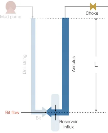
We consider the hydraulic part of a MPD drilling system composed of a drill string and an annulus through which flows a liquid, typically oil- or water-based mud. The open part of the annulus is in contact with a reservoir of uncer-tain pore pressure, permeability and porosity. This setup is schematically depicted on Figure 1. The liquid is injected at a known, variable flow rate using the mud pump at the surface and it is considered that the corresponding flow rate at the bit, qbit(t) is known. The topside part of the annulus
Fig. 1. Schematic of flow paths. For simplicity, the drill string and annulus are represented as a u-tube whereas, in reality, they are concentric.
is assumed to be sealed, which is the main feature of MPD operations, and the outflow is controlled via a choke valve. The main purpose of MPD is to improve the control of the BHCP compared to conventional drilling. Among the factors influencing the BHCP are regular operational transients, e.g. when the mud pump flow rate is decreased to zero during a connection, and unwanted incidents, e.g. when the choke is suddenly plugged, or when an unpredicted influx enters the wellbore from the reservoir. Here, we consider the case where a liquid influx is present, due to a reservoir pressure higher than anticipated. To accurately estimate the size of this influx, we model now the coupling between wellbore and reservoir dynamics.
A. Wellbore Model
We make the following simplifying assumptions: the flow is one dimensional, single-phase (liquid), temperature is constant. We denoteρ the liquid density and vl its velocity.
The liquid is assumed to follow the following Equation of State
p(t,x) = p0+ (ρ(t,x) −ρ0)C2l (1)
where Cl is the sound velocity in the liquid, t > 0 the
time variable and x ∈ [0,L] the spatial variable, where L is the total length of the pipe. The constants p0, ρ0 are
assumed to be perfectly known in drilling conditions. Writing mass and momentum conservation laws and assuming that
vl≪ Cl yields the following set of Partial Differential
Equa-tions (PDE) known as Euler’s equaEqua-tions,
qt+Aqx=S (2) where, A = !0 1 C2 l 0 " and S = ! 0 −F(q) − G(q) " , F(q) rep-resenting frictional pressure losses while G(q) accounts for gravity effects1. In what follows we denote
! q1(t,x) q2(t,x) " = ! ρ(t,x) ρ(t,x)v(t,x) " (3) B. Boundary conditions
At the inlet of the drill string, the flow rate is imposed by the pump. At the inlet of the annulus, the volumetric flow rate is given by
q2(t,0) =ρ0qbit(t) + qres(t)
A (4)
where A is the annulus area, qbit is the flow of drilling
fluid through the drill bit, given by a one-way-valve-like equation, and qres is the flow from the reservoir, which will
be discussed in the next section. The outflow is governed by a valve equation
Aq2(t,L) = KcZc(t)
# 2
q1(t,L)(p(q1(t,L),L) − pdc) (5)
where the downstream choke pressure pdc is assumed to be
constant and Kc is the choke constant and the flow area
through the choke depends on the choke opening Zc which
is the control input.
In the next section, we detail the model of the reservoir that enables computation of qres. We also give reduced
models typically used for reservoir characterization. C. Reservoir Model
We now derive the equations describing the pressure dynamics in the near-wellbore region of the reservoir. These correspond to the diffusion of hydrocarbons within porous rock. We then recall simplified models typically used in the literature for influx estimation, before making the case for the need to keep the distributed pressure dynamics.
1) Distributed model: We assume that the reservoir sec-tion is homogeneous and contains a single type of fluid, with no vertical diffusion. We then obtain the model from the linearized conservation of mass along with Darcy’s law relating flow rate to pressure [3]. We denote ϕ(r,t) as the pressure within the reservoir at a radial location r. The schematic of a radial section of the reservoir is given in Figure 2. The equations inside the radial domain of the reservoir r ∈ [rw,re]read
ϕt(r,t) =ar(rϕr(r,t))r (6)
1Notice that, although we do not consider the drill string here, this model
Fig. 2. Schematic of a radial section of the reservoir
where a =κ/(µctφ) is the diffusivity constant. The influx
into the wellbore (or loss) is obtained using, again, Darcy’s law and reads
qres(t) =ξϕr(rw,t) (7)
where, ξ = 2πκrwh/µ. Notice that the influx depends on
the pressure gradient at the boundary of the reservoir that coincides with the wellbore extent. Besides, the pressure in the reservoir at this boundary is assumed to coincide with the BHCP, which yields
ϕ(rw,t) = p(t,0) (8)
Equations (4),(7) and (8) are key as they summarize the coupling between the wellbore and reservoir. We now briefly review existing simplified reservoir models from the litera-ture and compare them with the full distributed model.
2) Simplified models: In [3] , the solution to equation (6) with various boundary conditions corresponding to situations arising in oil production is approximated. These lead to the so-called quasi-steady-state solution and constant terminal rate solution.
a) Quasi-steady-state solution: A first approximate so-lution can be obtained by assuming
• that the flux at the radial extent of the reservoir is null,
i.e.
ϕr(re,t) = 0 (9) • that the outflow from the reservoir is constant,
i.e. ˙qres=0.
Denoting qqssres the corresponding reservoir flow, this leads to
the following relation between the value of the pressure at the wellbore boundary, at the radial extent and the flow
qqss
res=−2πκhµ (ln(r(ϕ(rw,t) − pe)
e/rw)− 1/2) (10)
Although valid only for stabilized flow conditions, this relation, referred to as the PI relation, is sometimes used in a transient setting [8] or averaged over time [12].
0 5 10 15 20 25 30 0 0.5 1 1.5 2 2.5 3 3.5 10 -3
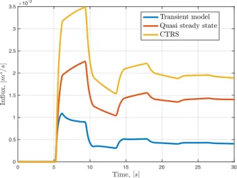
Fig. 3. Comparison of the three reservoir models
b) Constant terminal rate solution: Another approxi-mate solution is obtained by assuming
• that the radial extent of the reservoir is infinitely far
away, i.e. re=∞ and pressure is constant there, giving
the condition
lim
r→+∞ϕ(r,t) = pe (11) • that the flow rate qresis suddenly changed from zero to
a constant value
This yields the following relation between flow rate and pressure
qctr(t) = −4πκh(ϕ(rw,t) − pe)
µ$2Sk+lnγφ µc4κttr2w
% (12) This relation is the most widely used for reservoir charac-terization [9], [13].
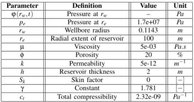
c) Comparison of reservoir models: Figure 3 depicts the influx flow rate resulting from these models and a comparison with the full distributed reservoir model (6) along with boundary conditions (8),(9). The scenario cor-responds to the liquid influx resulting from a reduction in BHCP caused by opening the choke. Table I summarizes the parameter values used for the simulation. The simulation shows that the influx is largely overestimated by the approx-imate models, because the conditions under which they are derived (constant flow rate or near-equilibria) are not satisfied in this transient situation. In the case of the quasi-steady-state solution, this is due to the fact that the distributed reservoir pressure reaches the quasi-steady-state only when the well has been producing for several weeks. This is the time needed for the pressure transient to reach the radial extent of the reservoir as described in [3].
Similarly, the constant terminal rate solution relies on a constant flow rate qres, which is a condition only satisfied
several weeks after the start of the production as mentioned in [3]. This type of solution is considered as a basic tool for wellbore pressure analysis that are helpful for the production engineers where the variation in flow rates are obtained
TABLE I
RESERVOIR PARAMETERS
Parameter Definition Value Unit ϕ(rw,t) Pressure at rw – Pa
pe Pressure at re 1.7e+07 Pa
rw Wellbore radius 0.1143 m
re Radial extent of reservoir 100 m
µ Viscosity 5e-03 Pa.s
φ Porosity 20 %
k Permeability 5e-12 m−1
h Reservoir thickness 2 m Sk Skin factor 0 [−]
γ Constant 1.781 [−]
ct Total compressibility 2.32e-09 Pa−1
by superposition of numerous constant terminal rate solu-tions [3]. In the interest of estimating influx flow rates while drilling, we are interested in the time period of at-most a few hours during which the transient behavior of the reservoir dominates.
In the next section, we derive an observer to estimate the distributed reservoir pressure relying on the measurement of BHCP and an observer to estimate the wellbore states relying on the measurement of surface choke pressure.
III. OBSERVERDESIGN
In this section, we highlight the structure of the coupling between the wellbore and the reservoir in view of influx estimation. We then present slight modifications of two ex-isting observer designs for the wellbore [2] and reservoir [6], respectively and show their potential for estimation through simulations.
A. Coupling boundary conditions
To highlight the structure of the coupling between reser-voir and wellbore, we rewrite the wellbore PDE (2) and the linearized form of the boundary conditions (4)–(8) in the Riemann coordinates (u,v)⊤given by
! u(t,x) v(t,x) " =1 2 ! Clq1(t,x) + q2(t,x) −Clq1(t,x) + q2(t,x) " (13) This yields a set of linear hyperbolic PDEs of the following form
ut(t,x) +Clux(t,x) =σ++(x)u(t,x) +σ+−(x)v(t,x) (14)
vt(t,x) −Clvx(t,x) =σ−+(x)u(t,x) +σ−−(x)v(t,x) (15)
where the σ·,· depend on the operating point around which
the equations are linearized. Simiarly, the choke equation (5) takes the following form
v(t,L) = ku(t,L) + kUZc(t) (16)
where k, kU depend, again, on the equilibirum around which
we linearize. At the reservoir boundary, Equations (4),(7) and (8) rewrite as u(t,0) = 1 Clϕ(rw,t) + v(t,0) (17) ϕr(rw,t) =Aξ ! 1ρ 0Clϕ(rw,t) + 2 ρ0v(t,0) − qbit(t) A " (18)
Under the form (17),(18), the boundary conditions give the structure of the coupling: the downward traveling pressure wave v influences the flux out of the reservoir and reflects into the upward traveling pressure wave. In turn, the reservoir pressure affects the upward traveling wave. This intercon-nection has a feedback structure that potentially generates instability. It is the case, e.g., when the pressure in the wellbore is significantly decreased by an influx of gas from the reservoir, since a larger pressure differential increases the flux. However, in the case considered here of a liquid influx, instability is unlikely as the density of the oil from the reservoir is very close to that of the drilling fluid. Thus, we assume in what follows that the interconnection is stable and design
• an observer for (14)–(17), assuming ϕ(rw,t) is known,
and relying on a topside choke pressure measure-ment pc;
• an observer for (6), assuming that v(t,0) is known,
relying on a BHCP measurement.
Fig. 4. Schematic of the combined observer design
This yields the observer structure depicted on Figure 4. We now detail the two designs.
B. Reservoir Observer
Considering BHCP as a measurement, y =ϕ(rw,t), and
assuming that the wellbore state v(t,0) is known, we consider the following standard Luenberger-like observer
ˆ ϕt(r,t) =ar(r ˆϕr(r,t))r+l(r)(y − ˆϕ(rw,t)) (19) ˆ ϕr(re,t) = 0 (20) ˆ ϕr(rw,t) =Aξ ! 1ρ 0Clϕ(rˆ w,t) + 2 ρ0v(t,0) − qbit(t) A " +l1(y − ˆϕ(rw,t)) (21)
where the observer gains l1 and l(r) are obtained using the
standard backstepping method [6] that provides l1=ξρA
0Cl+L(rw,rw)− K (22)
which are obtained by solving the PDE of gain kernel L(r,y) given by,
λ(y)Ly(r,y) + (C +λ′(y))L(r,y) + aLrr(r,y)
− aLyy(r,y) +λ(r)Lr(r,y) = 0 (24)
where, λ(r) = a/r. The exponential convergence of the resulting error system is proved by mapping it to an exponen-tially stable target error system using a Volterra coordinate transform as described in [6]. The design parameters C > 0 and K > 0 in the target system are degrees of freedom and can be used to achieve a trade-off between convergence speed, robustness and sensitivity to noise. This point is highlighted in Section IV
C. Wellbore Observer
Here, we slightly modify the design from [2], [1] to account for realistic measurements. Indeed, these designs as-sume that the boundary value of the Riemann invariant u(t,L) can be measured, which is not the case in practice. Rather, pressure sensors are typically available. Here, we generically assume that the measurement rewrites as a linear combina-tion of the Riemann invariants at the topside boundary, which yields
y = c1u(t,L) + c2v(t,L) (25)
In the case of the pressure measurement, one has c1=−c2=Cl. We then design, similarly to [2], [1], a
Luenberger-like observer as a copy of the plant plus linear output error injection which writes
ˆut(t,x) +Clˆux(t,x) =σ++ˆu(t,x) +σ+−ˆv(t,x)
− P+(x)(c1ˆu(t,L) + c2ˆv(t,L) − y) (26)
ˆvt(t,x) −Clˆvx(t,x) =σ−+ˆu(t,x) +σ−−ˆv(t,x)
− P−(x)(c2ˆu(t,L) + c2ˆv(t,L) − y) (27)
with the following boundary condition.
ˆv(t,L) = k ˆu(t,L) +εy −ε(c1ˆu(t,L) + c2ˆv(t,L) − y) (28)
ˆu(t,0) = 1
Clϕ(rw,t) + ˆv(t,0) (29)
where we assume that the reservoir boundary valueϕ(rw,t) is
known. Using the standard backstepping approach, the error system ( ˆu−u, ˆv−v) is mapped to the following target system αt(t,x) +Clαx(t,x) = 0 (30)
βt(t,x) −Clβx(t,x) = 0 (31)
with boundary conditions
β(t,L) =! k−εc1 1 +εc2 " α(t,L) (32) α(t,0) = β(t,0) (33) -1.5 -1 -0.5 0 0.5 1 10-3 -1 -0.8 -0.6 -0.4 -0.2 0 0.2 0.4 0.6 0.8 1
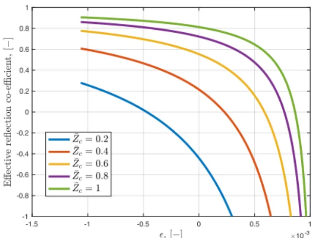
Fig. 5. Mapping of effective reflection coefficient as a function of the output error injection gain at the boundary, for different values of the choke opening.
provided the gains P+(x) and P−(x) satisfy
P+(x) =Cl(k − εc1)Puv(x,L) −Cl(1 +εc2)Puu(x,L)
c1(1 +εc2) +c2(k − εc1) (34)
P−(x) =Cl(k − εc1)Pvv(x,L) −Cl(1 +εc2)Pvu(x,L)
c1(1 +εc2) +c2(k − εc1) (35)
where Puu, Puv, Pvu, Pvv are the backstepping kernels
from [2]. Similarly to [1], the parameter ε is a degree of freedom. More precisely, we denote
¯k =! k−εc1
1 +εc2
"
(36) the effective reflection coefficient in the target system, which can be freely assigned using the design parameter ε. Im-posing ¯k close to zero yields a rapidly convergent observer. However, as indicated by (28), large values of ε tend to amplify measurement noise. Importantly, a necessary and sufficient condition for the stability of (30)–(33) is that ¯k satisfy
−1 < ¯k < 1 (37) Notice that the value of k, that comes from the linearization of the choke equation (5), varies according to the equilibrium that, itself, depends on the choke opening. It is possible to change the value of ε according to the choke opening to maintain a constant effective reflection coefficient ¯k through-out the operation, but a time-dependent coefficient induces additional dynamics that may lead to instability. Rather, it is possible to map the value of ¯k throughout the operating range and chose a constant epsilon that ensures that (37) is satisfied for all values of Zc. This is the point illustrated on
Figure 5.
IV. SIMULATIONS
In this section, we study the coupled observer designed according to the structure depicted on Figure 4. In practice, the estimate ˆv(t,0) from the wellbore observer is inserted
TABLE II
WELLBORE PARAMETERS
Parameter Definition Value Unit qbit Flow rate at bit 0.03 m3s−1
L Length of the wellbore 2000 m Kc Choke constant 2.85e-03 [−]
¯Zc Steady state choke opening 0.95 [−]
Cl Velocity of sound 940.30 m.s−1
p0 Reference pressure 1e+05 Pa
ρ0 Reference density 780 kg.m−3
in (21) and the estimate ˆϕ(rw,t) from the reservoir observer
is inserted in (18) for the reservoir and wellbore observers respectively. We consider various industry relevant scenarios to study the performance and robustness of this combined observer design. Table II summarizes the simulation param-eters.
A. Drilling into a high pressure pocket
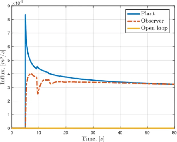
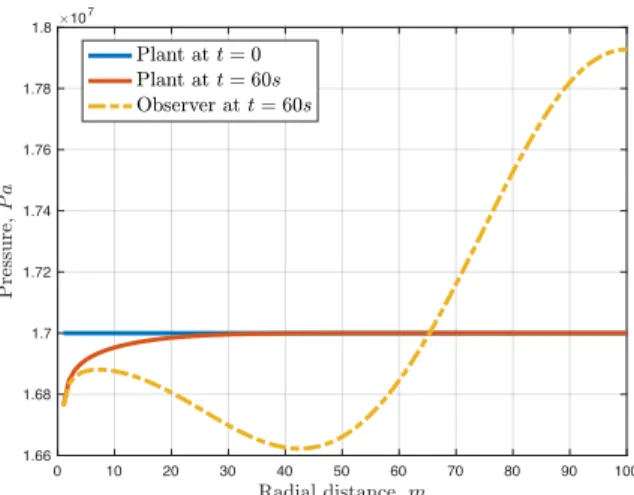
During drilling, it is common to encounter pockets of hydrocarbons with higher pressure than anticipated. Drilling into such zones will lead to an influx. We present here a case where a section with known reservoir pressure is drilled using MPD and a high pressure pocket is encountered at 5s. The pressure within the pocket is considered to be 50% higher than that of the anticipated. As depicted on Figure 6, the observer successfully estimates the influx, while no influx is detected in the absence of an observer (i.e. in open loop). The near wellbore reservoir pressure distribution is also estimated by the observer as shown on Figure 7. Interestingly, the reservoir pressure is poorly estimated away from the wellbore but this does not affect the influx estimation.
0 10 20 30 40 50 60 0 1 2 3 4 5 6 7 8 9 10 -3
Fig. 6. Influx estimation by the observer in comparison to the plant measurement and in the absence of an observer for case–A.
B. In presence of transients
During MPD operation, there are instances when the choke opening is varied rapidly in order to maintain the required BHCP. We present the case here with an over estimation
0 10 20 30 40 50 60 70 80 90 100 1.5 1.6 1.7 1.8 1.9 2 2.1 2.2 2.3 2.4 2.5 10 7
Fig. 7. Time snapshots of distributed pressure profile within the reservoir obtained from plant in comparison to that of the estimation by the observer for case–A.
of the reservoir and wellbore parameters to emulate the uncertainty of these parameters in practice, inclusive of tran-sients introduced by the choke variations. The perturbation of wellbore states from the steady state profile, reservoir pressure and permeability are assumed to be overestimated by 10% each and Zc varied from 0.8 to 0.4 in 1s. Despite
the uncertainty in the reservoir and wellbore parameters, the observer successfully estimates the influx and the near well-bore reservoir pressure distribution as depicted in Figures 8 and 9 respectively. 0 5 10 15 20 25 30 0 0.5 1 1.5 2 2.5 3 3.5 10 -3
Fig. 8. Influx estimation by the observer in comparison to the plant measurement for case–B.
V. CONCLUSIONS AND FUTURE WORKS
We have presented a reservoir model capturing the dis-tributed properties of the pressure dynamics in view of influx estimation. Applying existing observer designs for the wellbore and reservoir dynamics enables estimation of the influx flow rate despite uncertainty on the reservoir characteristics. This first step opens a large perspective of future works.
0 10 20 30 40 50 60 70 80 90 100 1.66 1.68 1.7 1.72 1.74 1.76 1.78 1.8 10 7
Fig. 9. Time snapshots of distributed pressure profile within the reservoir obtained from plant in comparison to that of the estimation by the observer for case–B.
First, a coupled parabolic–hyperbolic observer could be designed, which would be a novel result in control and estimation of PDEs. Modifying the backstepping transforma-tions such that the entire wellbore-reservoir state is mapped to a stable target system induces nonlinear, nonlocal relations between the backstepping kernels, which severely compli-cates the proof of their well-posedness.
Most importantly, influxes of fluids with densities varying from the drilling fluid need to be considered and modeled. This drastically modifies the wellbore dynamics, in particular if gas is present. This is a key direction for future work. Another important modelling aspect is to deal with the potential longitudinal heterogeneity of the reservoir in the open section of the well.
REFERENCES
[1] Jean Auriol, Ulf Jakob Fl Aarsnes, Philippe Martin, and Florent Di Meglio. Delay-robust control design for heterodirectional linear coupled hyperbolic pdes. IEEE Transactions on Automatic Control, 2018.
[2] Jean-Michel Coron, Rafael Vazquez, Miroslav Krstic, and Georges Bastin. Local exponential h2 stabilization of a 2× 2 quasilinear
hyperbolic system using backstepping. SIAM Journal on Control and Optimization, 51(3):2005–2035, 2013.
[3] LP Dake. Fundamentals of reservoir engineering., 1978, 1983. [4] Stein Hauge and Knut Øien. Deepwater horizon: Lessons learned
for the norwegian petroleum industry with focus on technical aspects. Chemical Engineering, 26, 2012.
[5] Wendy Kneissl et al. Reservoir characterization whilst underbalanced drilling. In SPE/IADC drilling conference. Society of Petroleum Engineers, 2001.
[6] M. Krstic and A. Smyshlyaev. Boundary Control of PDEs. SIAM Advances in Design and Control, 2008.
[7] Scott J Moura, Nalin A Chaturvedi, and Miroslav Krsti´c. Adaptive partial differential equation observer for battery state-of-charge/state-of-health estimation via an electrochemical model. Journal of Dynamic Systems, Measurement, and Control, 136(1):011015, 2014.
[8] Amirhossein Nikoofard, Tor Arne Johansen, and Glenn-Ole Kaasa. Design and comparison of adaptive estimators for under-balanced drilling. In American Control Conference (ACC), 2014, pages 5681– 5687. IEEE, 2014.
[9] G. H. Nygaard, E.H. Vefring, K.-K. Fjelde, G. Næ vdal, and Lorentzen R. J. Bottomhole pressure control during drilling operations in gas-dominant wells. SPE Journal, 12(1):49–61, March 2007.
[10] Alexey Pavlov and Glenn-Ole Kaasa. Statoil: Automatic mpd a coming reality. Drilling contractor, 67(4), 2011.
[11] Andrey Smyshlyaev and Miroslav Krsti´c. Explicit state and output feedback boundary controllers for partial differential equations. Jour-nal of Automatic Control, 13(2):1–9, 2003.
[12] PV Suryanarayana, Ravimadhav N Vaidya, Jan Wind, et al. Use of a new rate-integral productivity index in interpretation of underbal-anced drilling data for reservoir characterization. In Production and Operations Symposium. Society of Petroleum Engineers, 2007. [13] Erlend H Vefring, Gerhard H Nygaard, Rolf J Lorentzen, Geir
Naevdal, Kjell K Fjelde, et al. Reservoir characterization during underbalanced drilling (ubd): methodology and active tests. SPE Journal, 11(02):181–192, 2006.