HAL Id: hal-02348464
https://hal.archives-ouvertes.fr/hal-02348464
Submitted on 20 Jan 2021HAL is a multi-disciplinary open access
archive for the deposit and dissemination of sci-entific research documents, whether they are pub-lished or not. The documents may come from teaching and research institutions in France or abroad, or from public or private research centers.
L’archive ouverte pluridisciplinaire HAL, est destinée au dépôt et à la diffusion de documents scientifiques de niveau recherche, publiés ou non, émanant des établissements d’enseignement et de recherche français ou étrangers, des laboratoires publics ou privés.
Fast quantitative 2D NMR for metabolomics and
lipidomics: A tutorial
Estelle Martineau, Jean-Nicolas Dumez, Patrick Giraudeau
To cite this version:
Estelle Martineau, Jean-Nicolas Dumez, Patrick Giraudeau. Fast quantitative 2D NMR for metabolomics and lipidomics: A tutorial. Magnetic Resonance in Chemistry, Wiley, 2019, �10.1002/mrc.4899�. �hal-02348464�
Fast quantitative 2D NMR for metabolomics and lipidomics: a
tutorial
Estelle Martineau1,2, Jean-Nicolas Dumez1 and Patrick Giraudeau1,3,*
1 EBSI Team, CEISAM, 2 rue de la Houssinière, BP 92208, 44322 Nantes Cedex 3, France
2 SpectroMaitrise, CAPACITES SAS, 26 bd Vincent Gâche, 44200 Nantes, France
3 Institut Universitaire de France, 1 rue Descartes, 75005 Paris Cedex 5, France
Fast quantitative 2D NMR for metabolomics and lipidomics: a
tutorial
Estelle Martineau1,2, Jean-Nicolas Dumez1 and Patrick Giraudeau1,3,*
Nuclear Magnetic Resonance (NMR) has a great potential for the quantitative analysis of complex biological samples. The acquisition of 2D NMR spectra allows a better separation between overlapped resonances while yielding accurate quantitative data when appropriate analytical protocols are implemented. The experiment duration can be made compatible with high-throughput studies by relying on fast acquisition methods. This tutorial describes the general workflow to acquire fast quantitative 2D NMR data for metabolomics and lipidomics applications.
Fast quantitative 2D NMR for metabolomics and lipidomics: a
tutorial
Estelle Martineau, Jean-Nicolas Dumez and Patrick Giraudeau
Abstract
Nuclear Magnetic Resonance (NMR) is a well-known analytical technique for the analysis of complex mixtures. Its quantitative capability makes it ideally suited to metabolomics or lipidomics studies involving large sample collections of complex biological samples. To overcome the ubiquitous limitation of spectral overcrowding when recording 1D NMR spectra on such samples, the acquisition of 2D NMR spectra allows a better separation between overlapped resonances while yielding accurate quantitative data when appropriate analytical protocols are implemented. Moreover, the experiment duration can be considerably reduced by applying fast acquisition methods. Here, we describe the general workflow to acquire fast quantitative 2D NMR spectra in the “omics” context. It is illustrated on three representative and complementary experiments: UF COSY, ZF-TOCSY with non-uniform sampling and HSQC with non-uniform sampling. After giving some details and recommendations on how to apply this protocol, its implementation in the case of targeted and untargeted metabolomics/lipidomics studies is described.
Key words 2D NMR spectroscopy, quantitative analysis, fast methods, metabolomics,
Fast quantitative 2D NMR for metabolomics and lipidomics: a
tutorial
Introduction
Nuclear Magnetic Resonance (NMR) spectroscopy is a well-known and powerful analytical technique, which is widely used for structure elucidation. This technique, which is highly repeatable and non-destructive, has also proven its ability to quantify analytes in mixtures, most often with the use of 1D 1H NMR. Unfortunately, in the case of complex mixtures, 1D 1H NMR suffers from numerous peak overlaps that limit its usefulness as a quantitative tool in several applications: in fact, the quantification of compounds can be difficult or even impossible when no isolated peak can be found for the analyte of interest.
Two-dimensional NMR is one of the solutions to overcome the overlap problem. 2D NMR offers a much better discrimination of resonances as the peaks are spread along an additional dimension. The availability of a broad variety of homonuclear and heteronuclear pulse sequences is a major advantage of 2D NMR experiments, since these have different levels of resolution and sensitivity. However, 2D NMR experiments suffer from two main drawbacks that make their use for quantitative analysis not straightforward. The first one is long experiment durations, which result from the need to repeat numerous 1D sub-experiments in order to obtain 2D spectra with sufficient resolution. Experiment durations can reach several hours per spectrum, which is incompatible with many applications such as metabolomics, which requires high-throughput methods to analyze large sample collections. In addition, long experiments are more sensitive to spectrometer instabilities, which affect the precision of quantitative measurements. Fortunately, numerous approaches have been suggested to reduce experiment durations[1]. Although these methods are associated with sensitivity losses and/or resolution penalties these limitations are well described and understood. Two of these methods (Non-Uniform Sampling or NUS and UltraFast (UF) NMR) have successfully been used in targeted and untargeted metabolomics and lipidomics workflows[2],[3],[4],[5],[6].
The second drawback of 2D NMR for quantitative analysis is linked to the multi-pulse nature of 2D NMR experiments, which results in a peak-dependent analytical response of the nuclei[7]. In other words, 2D NMR peak volumes are still proportional to analyte concentrations –as is the case in 1D NMR– but the coefficient of proportionality between the peak volume and the concentration is different for each peak in the spectrum. This coefficient of proportionality depends on peak-specific factors such as homo/hetero-nuclear J-coupling constants and transverse relaxation times. Consequently, several strategies have been developed to yield accurate analyte concentrations from 2D spectra (Figure 1). The development of specific pulse sequences has led to a peak-independent coefficient of proportionality between the 2D NMR signal and the concentration, hence to pulse sequences that are “intrinsically” quantitative such as HSQC0[8], Q HSQC[9],[10] or Q QUIPU HSQC[11]. These promising methods are still limited
in terms of accuracy, yielding an average trueness of 10%[11]. Theoretical correction for
relaxation during 2D pulse sequence has also been introduced by Rai et al. to quantify metabolites in urine samples[12]: this option is mentioned regularly but is not applied in practice in the literature, probably because of the practical impossibility to accurately determine correction factors in complex mixtures. Another strategy consists in calibrating the 2D peak
response as a function of concentration for all the targeted analytes, relying on an analytical chemistry approach such as an external calibration[13],[14] or a standard addition procedure[15]. All the targeted analytes can be quantified simultaneously provided that standards of known purity are available –which is often the case for common metabolites detectable by NMR. This strategy yields a very high trueness and precision of a few percent.
Fast quantitative 2D NMR methods are particularly relevant to the fields of metabolomics and lipidomics. NMR spectroscopy has become a technique of choice for metabolomics over the past fifteen years, and it is used both as an untargeted method to record a fingerprint of complex biological samples (biofluids, extracts, food matrices, etc.) and as a targeted method to determine the concentration of multiple analytes in such complex samples. While the most widely used approach is 1D 1H NMR, its applicability is often limited by the spectral crowding issues described above. That is why 2D NMR methods have been introduced in the field of metabolomics and lipidomics, and more precisely fast 2D NMR[4],[5],[6],[16]: indeed, the reduced experiment duration is compatible with high- throughput studies[19][17], the experiments are more repeatable if they are shorter and they are compatible with a potential sample evolution over time.
This tutorial describes a general protocol to apply fast quantitative 2D NMR experiments in the “omics” context. The pulse sequences used here are well described in the literature, and we focus on their use to quantify analytes with calibration approaches[18]. We start with the presentation of some important technical aspects, as well as an initial evaluation describing how to decide which pulse sequence to use, including acquisition and processing parameters. Then, we detail how to apply this protocol for a metabolomics or lipidomics study. While the tutorial uses three specific sequences as illustrations, the corresponding protocol can be applied to other 2D NMR sequences (with and without fast acquisition strategies).
Equipment
Although the workflow described in this tutorial is not field-dependent, for applications to biological samples, we recommend the use of a high-field spectrometer, with a probe equipped with a z-axis magnetic-field gradient. For metabolomics applications, NMR spectrometers in the 500-800 MHz range offer a good performance in terms of sensitivity and separation of the signals of interest. Having a cryogenically cooled probe will be a plus if the concentration of samples is quite low (a few dozens µmol.L-1), but it can also be detrimental for samples with
high salinity. If an automatic sample changer is available on the spectrometer, its use will be compatible with fast quantitative 2D NMR; a refrigerated high capacity one will be a plus to analyze big cohorts of samples and/or samples which could suffer from damages if they are kept for too long at ambient temperature. High quality tubes should be preferred. While samples are generally analyzed with 5 mm NMR tubes, if the quantity of samples is too small, the samples can be analyzed with 3 mm NMR tubes.
Sample preparation for NMR
The collection and the preparation of biological samples for NMR analysis have already been described in the literature in several protocols[19], depending on the type of sample analyzed
(urine, blood, extracts, tissues, etc.). Here, we will highlight some particular points of the sample preparation in the case of metabolomics studies:
• The appropriate extraction protocol should be chosen according to the aim of the study, depending if the entire or a specific fraction of the metabolome (lipids, polar metabolites, etc.) is targeted;
• For biological extracts or samples sensitive to pH variation, a buffer can be used in order to avoid a deviation of chemical shifts due to pH variation;
• Particular attention should be paid to the tubes used to take blood or serum, as they can contain EDTA, citrate or other added stabilizers which give additional signals on NMR spectra[20];
• Some Quality Control samples (QCs) should be prepared when the design of the studies allows it: these samples consist of all the collected biological samples pooled in identical quantities mixed together. QCs can be used to regularly check the quality of the analysis; • The samples should be stored between -80°C and -20°C before NMR preparation[21].
Before starting the NMR preparation, samples are thawed (15-30 minutes), then solvent(s) are added into the vial[19]:
• If the samples are in the solid state, between 600 µL and 700 µL of deuterated solvent (and/or buffer) should be added[5],[6], or a mix of deuterated and non-deuterated solvents respecting the proportions of 80%/20% or 90%/10%. At least 20 mg of biological sample (wet mass) are necessary to acquire NMR spectra in a reasonable time –a mass of 100 mg of biological is the typical size for this kind of analysis[19]. However, particular attention must be paid to the sample solubility in the chosen solvent (preliminary tests can be necessary);
• If the samples are in the liquid state and if possible, a ratio of 80%/20% for sample/deuterated solvent (and/or buffer) for a total volume of 700 µL should be used: in that case, 500 µL of biological sample is the best to acquire spectra in a reasonable time. The analyses are still possible with less sample, but they potentially will last longer;
• The addition of a reference is recommended to calibrate the chemical shift scale for all the spectra[17]: this is particularly important for the untargeted approach to ensure that the spectra are stackable for the bucketing part, and this signal can also be used for the normalization part.
The chemical shift of the chosen reference must not overlap with a signal of interest: for instance, the signal of TrimethylSilylPropanoic acid (TSP, which is soluble in D2O) or
TetraMethylSilane (TMS, which is soluble in organic solvents such as CDCl3 but
evaporates above 26°C) has the advantage to be at 0 ppm, where there is no other signal of interest. According to the targeted accuracy, the use of a silicon reference may be avoided because of the silicon satellites. In the case of lipidomics, DiMethyl SulfOne (DMSO2, which is soluble in organic solvents such as CDCl3) can be an appropriate
reference as its signal is a singlet at a chemical shift of 3 ppm: prior to addition of DMSO2 inside each sample, it should be verified that there is no signal of interest close
to this region.
The concentration of the reference compound should be chosen to set its NMR signal intensity to a value smaller than or equal to that of the most intense signal of interest: indeed, as the receiver gain (RG) of the NMR experiments is set according to the most
intense signal, if the concentration of the reference is too large, its NMR signal intensity determines the value of the receiver gain and the detection of the signals of interest is not optimal;
• In the case of the targeted approach, and after identifying the metabolites of interest, a stock solution containing the targeted metabolites in known concentrations has to be prepared. In the specific case of standard additions, this stock solution should be concentrated in order to add a small volume (≤ 10 µL) to avoid diluting the analyzed samples.
After solvent addition, the samples are vortexed and put inside NMR tubes. The samples should be stored at -20°C before analysis:
• If an automatic sample changer cannot be used, all samples must not be thawed at the same time, but only the analyzed one, usually 15 minutes before vortexing and insertion into the magnet;
• If an automatic sample changer can be used, a preliminary evaluation of sample stability is necessary in order to be sure that the sample does not evolve in time at the temperature of the sample changer (refrigerated or not). In order to mimic a potential long stay of a sample prior to the insertion inside the magnet, stability studies at both ambient and refrigerated temperatures should be carried out, recording a 1D 1H spectrum for each
hypothesis tested. The choice to use or not an automatic sample changer will be made according to what can be observed on NMR spectra, and also depending on the number of samples.
NMR experiments
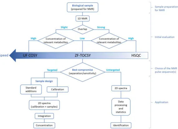
Before analyzing a cohort of samples, an initial evaluation is required to determine which NMR pulse sequence(s) are appropriate to answer the biological question of interest (Figure 2). In this entire chapter, we assume that 2D spectra can be recorded under partial saturation conditions (i.e., with a recovery delay shorter than 5 times the longest longitudinal relaxation time T1) if the experiment duration is a critical factor. Indeed, unlike 1D NMR, where respecting
this condition is critical to ensure that the coefficient of proportionality between peak areas and concentrations is the same for all the peaks in the spectrum, this condition is not required for 2D NMR spectra combined with calibration or standard addition approaches. In 2D NMR, the effect of T1 is one factor among others (T2, coupling constants) affecting the coefficient of
proportionality between peak volumes and concentrations. Therefore, partial saturation conditions remain compatible with the approach described in this chapter, at the condition that T1 values do not vary significantly between samples in a study[7]. Note that partial saturation is
not compatible with “intrinsically” quantitative 2D methods of the HSQC family, which are, however, out of the scope of this chapter.
Initial evaluation
1. Settings and acquisition parameters common to all pulse sequences
First, start by the analysis of a representative sample in the cohort (for example a control one or a QC). After thawing (an average 15-30 minutes) and vortexing, the sample can be introduced inside the magnet. The choice of the temperature of analysis must be done according to the nature of the analyzed sample and/or the chosen solvent: for instance, 298 K or 300 K are common temperatures in the literature[18][19]. After waiting typically 10-15 minutes in order to ensure thermal stability of the sample, the adjustment of the field-frequency lock and the magnetic field homogeneity (lock and shim) should be carefully made before NMR acquisition. A 1D 1H spectrum is acquired in order to verify the quality of shimming and to determine some important parameters needed before acquiring 2D homonuclear spectra on all the samples of the cohort:
• The spectral width and the frequency offset must be adapted according to the chemical shifts of the biological samples;
• The saturation of the solvent signal can be necessary: applying a solvent saturation is generally required if the solvent signal is significantly more intense than the peaks of interest and/or overlaps with targeted peaks[22]. In that case, the parameters of the solvent suppression pulse sequence should be adapted to decrease the solvent signal as much as possible without disturbing the baseline and affecting nearby peaks. Thus, one should try to reduce the solvent signal intensity to a value smaller than the most intense signal of interest in order to set a receiver gain adapted to the sample. Moreover, the frequency offset of saturation must be adjusted to the exact position of the solvent peak: on cryogenically cooled probes, this parameter may require empirical optimization to improve solvent suppression. Note that several solvent suppression techniques are suitable for metabolite samples; an approach to evaluate the efficiency of the different methods for a given sample is described in Ref. [22]. Also note that solvent saturation can be avoided or reduced to a low power if exchangeable protons need to be observed; • A careful calibration of the hard power 90° pulse duration is necessary. Then, this value should be kept constant for all the experiments: in fact, the pulse duration is not expected to vary for a series of biological samples prepared in the same conditions.
Then, a collection of typical 2D spectra can be acquired: this is necessary to choose the most appropriate one for the entire study. As numerous pulse sequences are available, we will recommend to record at least one homonuclear 2D 1H experiment, with or without solvent
saturation, either an ultrafast COSY[23] (≤ 30 minutes – Figure 3 a and d) or a Z Filtered TOCSY (ZF-TOCSY – Figure 3 b and e) with 50% of Non-Uniform Sampling (NUS)[4], [24], as well as
an heteronuclear 1H-13C HSQC experiment with 25% of NUS (Figure 3 c and f)[4]. We detail some specific parameters for each pulse sequence in paragraph 2 and focus here on those which are common to all pulse sequences.
More particularly, it is recommended to pay attention to:
• The receiver gain. It can be automatically calculated as for 1D experiments, on condition that a relaxation delay of at least 5 s is chosen for UF COSY to limit the demand on the gradient coil and amplifier. For NUS experiments, a 1D version of the 2D experiment should be used to set the receiver gain;
• The number of scans. Its value has to be a multiple of 2 for all the pulse sequences mentioned above and should be optimized in order to reach a signal-to-noise ratio (SNR) greater than or equal to 10 for the signals of interest (Limit Of Quantification or LOQ). For UF COSY, this value must take into account a 30-minute maximum value for the experiment duration, in order to avoid damage of the gradient coil;
• The recovery delay. Its value should be optimized according to the dedicated time allotted to the analysis of the whole cohort, remembering that partial saturation is in principle not an issue;
• The acquisition time. Its value is calculated automatically for UF COSY experiments (see the online protocol for the implementation of ultrafast 2D NMR experiments [25]). For ZF-TOCSY experiments, Thrippleton et al. recommend a value of 1 s[24]. For HSQC experiments, the acquisition time should be between 0.2 s and 0.4 s;
• The use of dummy scans is recommended: the values suggested by Topspin can be used for HSQC and ZF-TOCSY experiments (DS = 16). For UF COSY experiments, the number of dummy scans is set at 2.
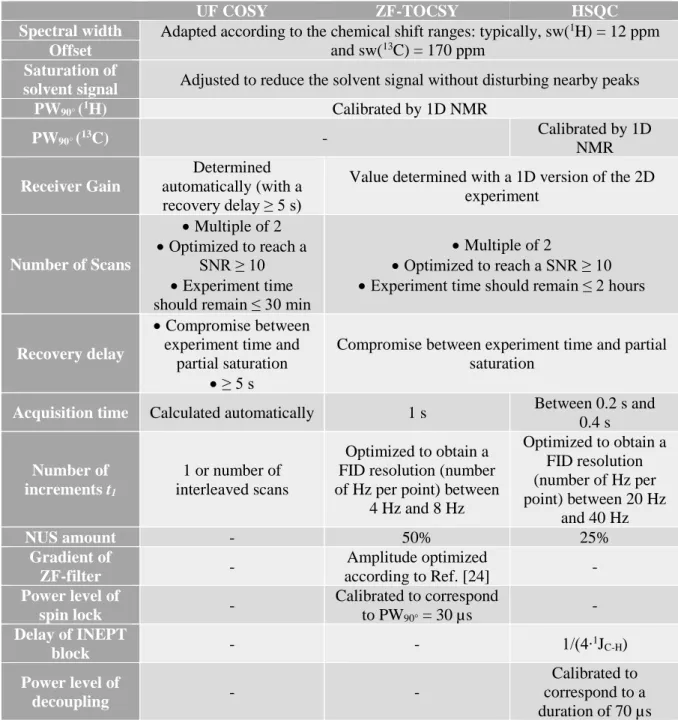
Thanks to this initial evaluation, the values of the receiver gain and the number of scans are now optimized for the untargeted approach. These values must be adjusted on the most concentrated sample (for the receiver gain) and the less concentrated one (for the number of scans) for the targeted approach (see below in the application part). Major acquisition parameters are described in Table 1.
2. Acquisition parameters specific to each pulse sequence 2.1. UF COSY
The acquisition and processing parameters to use for the UF COSY pulse sequence are described in a protocol available online[25]. This protocol explains the different steps to follow in order to implement correctly ultrafast 2D NMR experiments; in particular, for UF COSY experiments, the main parameters which have to be optimized and/or used to acquire spectra are listed. It also underlines some traps to avoid.
Some particular attention should be paid to the dispersion induced by the gradients and the calibration of the encoding pulses. These preliminary calibrations consist in calibrating the gradients and the chirp pulse and are necessary to characterize hardware performances before acquiring UF COSY spectra.
2.2. ZF-TOCSY
The acquisition and processing parameters to use for the ZF-TOCSY with 50% of NUS are described in recent articles[4],[24]. The classical TOCSY pulse sequence is improved by the addition of a Z-Filter in order to dephase zero quantum coherence, and applying the spin-lock while the magnetization is along the z-axis ensures a better sensitivity. The corresponding pulse sequence is provided as supplementary information. Before acquiring ZF-TOCSY spectra, the parameters of this Z-filter, and more precisely the amplitude of the gradients, must be optimized with the protocol of Thrippleton and Keeler[24]. The power level to be used during the spin lock of the ZF-TOCSY pulse sequence should be calibrated to correspond to a 90° pulse duration of 30 µs. If possible (depending on time constraints), the number of increments t1 should be
acquisitions of NMR spectra without losing too much sensitivity (NB: NUS can also be used to record very high resolution spectra without compromising on the experiment time[26]).
2.3. 1H-13C HSQC
Before obtaining 2D HSQC spectra on all the samples of the cohort, 1D 13C spectra (with 1H decoupling) should be acquired in order to determine some important parameters needed:
• The spectral width and the frequency offset must be adapted according to the chemical shifts of the biological samples;
• The duration of the hard power 90° pulse must be calibrated. Then, this value should be kept constant for all the experiments: no significant variation is expected for a series of biological samples prepared in the same conditions. Quaternary carbons can be ignored in this calibration procedure since they will not be observed in the HSQC spectrum; • The calibration of the power level corresponding to the duration of a 13C decoupling
pulse of 70 µs must be carried out.This duration will be used in a program adapted to the decoupling of 13C nuclei (such as GARP or GARP4).
The approach is compatible with any of your favorite routine HSQC pulse sequence. The acquisition and processing parameters to use for the HSQC 1H -13C pulse sequence with 25% of NUS are described in recent publications[4]. If the spectral width is too large, spectral aliasing can be applied in the indirect dimension (13C chemical shift)[27],[28]. In this case, particular
attention should be paid to the value of the corresponding frequency offset: a frequency change during the pulse sequence must be operated so that the frequency offset is in the middle of the aliased range during the evolution period (when t1 is incremented) and so that the frequency
offset is in the middle of the entire 13C range (without aliasing) during the rest of the experiment. If possible (depending on time constraints), the number of increments t1 must be adjusted to
obtain a FID resolution between 20 Hz and 40 Hz. The delays of the INEPT blocks depend on the average constant value 1JC-H: if this value cannot be determined a priori, we suggest using
a typical value of 145 Hz. The classical HSQC pulse sequence is improved by the use of 25% of NUS (ie. only 25% of the points are actually recorded), which allows faster acquisitions of NMR spectra without losing too much sensitivity. Although much stronger NUS conditions have been suggested in the literature, the TD1 and AQ values suggested here do not allow setting the percentage of NUS below 25%.
3. Processing parameters
After acquisition of the different 2D spectra, the processing parameters must be adjusted to the analyzed samples. The time-domain data can be multiplied by the appropriate apodization functions before applying the Fourier transform operation. Several such functions exist (exponential, gaussian, sinusoidal, etc.), and the choice of the appropriate apodization functions depends on the pulse sequence, and should be made to obtain the best compromise between sensitivity and separation of the signals of interest. If needed, phase-correction parameters in each dimension can be adjusted manually. For UF COSY, a dedicated automation program is available to process the data with appropriate processing parameters (including apodization in the spatially-encoded dimension) and display the resulting spectra. For experiments using NUS, the use of the Iterative Reweighted Least-Square (IRLS) algorithm is recommended[29] (here, the experiments were processed with 20 iterations (mdd_csniter = 20). Moreover, a Hilbert transform must be applied in the direct dimension to be able to phase the indirect dimension.
Then, a baseline correction can be applied in both dimensions: the degree of the polynomial baseline correction should be optimized depending on the baseline distortions observed on the row and column projections. A default value of 2 is recommended in both dimensions. Major processing parameters are described in Table 2.
Then, the spectra are calibrated on the chemical shift of the internal reference: this step is important in order to use the same bucketing or integration file for each spectrum (see below). Note that the calibration of UF COSY spectra requires two distinct peaks; typically the peak of the reference and another peak whose chemical shift is not varying throughout the samples. Ideally, all the spectra should be stackable after calibration of the chemical shift axis. In practice, when the samples are not buffered (e.g. urine or plasma) or do not have exactly the same pH, the calibration cannot lead to a perfect superposition of all the spectra. In this case, the position of the buckets or integration regions must be automatically or manually adjusted – without changing their size.
After processing all the spectra, the bucketing or the integration can be applied to all the signals of interest with SNR ≥ 10, including, for homonuclear experiments, diagonal signals that are well separated from the other signals. Typically, integration boxes are drawn –for instance rectangles with AMIX (Aurelia/Bruker) or Topspin (Bruker), or ellipses with MestReNova (Mestrelab Research)– around the signals of interest. Particular attention must be paid to the size of the rectangles: they have to be large enough to include most of the signal but not too large, so as not to include another nearby signal or, in the case of magnitude spectra, additional noise. We recommend modifying the contour plot level to be sure that the integration box matches the signal of interest without integrating a nearby peak. If some doubt exists, it is better to draw a smaller box than a too large one. With the AMIX software, the boxes can be defined on all spectra at the same time whereas with Topspin or MestReNova software, they must be defined on one of the spectra, then applied to the others. In this case, the corresponding file must be named and saved, then recalled on each spectrum to pick up the values of integration areas. Once all the boxes are drawn, a spreadsheet file is created to collect all the “raw” integration values associated to each bucket or integration region, i.e., without applying any normalization at this stage.
Sometimes, the signals of some metabolites can be overlapped; applying a symmetrization on a homonuclear spectrum can help to identify the metabolites, but the symmetrized spectrum must not be used for the bucketing part or the quantification part.
Choice of the NMR pulse sequence(s)
The choice of the pulse sequence(s) depends on the biological question of interest and a compromise is often necessary to achieve the best separation of the signals of interest and the sensitivity needed to detect the metabolites of interest within the allotted time. This time has to be compatible with high-throughput metabolomic studies, i.e. analyzing a maximum of samples in the minimum of time. The person in charge of the experimental design should carefully define the goal of the study: does it aim at obtaining a maximum of information (= untargeted approach/profiling) or rather accurate information on a limited number of concentrated metabolites (= targeted approach)? In the case of untargeted approaches, the approach allowing the detection of the greatest number of metabolites in the minimum of time with a sufficient sensitivity will be preferred. In the case of targeted approach, one should focus on detecting,
one signal well separated from the others for each metabolite of interest. These signals will be used for the quantification.
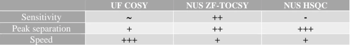
Table 3 summarizes the pros and cons for each NMR pulse sequence presented here. Moreover, with the upper part of Figure 2, one can easily select the most appropriate sequence pulse sequence to analyze a cohort of biological samples.
For instance:
• if spectra present an overlap in 1D NMR that can be solved by homonuclear 2D NMR,
and if the concentration of the relevant metabolites is high enough, applying the UF COSY sequence will be a good compromise, especially if time is critical due to a high number of samples or to sample unstability;
• if spectra present a strong overlap by 1D NMR and if the concentration of relevant metabolites is high enough, applying HSQC experiment with NUS will lead to an optimal separation of overlapping signals;
• if the concentration of relevant metabolites is low, applying ZF-TOCSY pulse sequence will be a good compromise to obtain separated signals with a reasonable sensitivity. According to these recommendations, the most appropriate pulse sequence(s) must be selected. In order to be in the same experimental conditions for each sample, it is suggested to create a file containing the acquisition and processing parameters, which will be recalled for the analysis of the cohort, and to record also a shim file.
Application: untargeted and targeted approaches
As explained above, with 2D NMR, the coefficient or proportionality between peak volume and concentration is different for each signal in the spectrum. For the untargeted method, relative peak intensities are compared from one sample to another. Thus, 2D peak volumes can still be used for the intercomparison of samples, provided that all the samples are prepared in similar conditions[31]. For the targeted method, we will only focus here on the calibration approaches, i.e., standard addition procedure[15] and external calibration[13],[14].
1. Untargeted approach
The different steps of the untargeted approach are presented in Figure 4. 1.1. NMR analysis
The first step consists of the acquisition of 2D spectra on all the samples of the cohort: they should be analyzed in a randomised order in order to limit effects on the final results. For this step, the samples must be thawed (15-30 minutes) and vortexed before insertion inside the magnet. If an automatic sample changer cannot be used, samples should be thawed only one at a time. If a refrigerated automatic sample changer is available, all or a part of the samples can be inserted inside at a temperature of 4° C. Moreover, and if allowed by the sample changer, the following sample must be automatically pre-heated at the analyzed temperature prior to the insertion inside the magnet (10 minutes on average). After waiting 10 minutes in order to ensure thermal stability of the sample, the system must be locked (automatic); the shim file recorded previously can be called on the first sample and the automatic setting of shims can be applied.
When all the settings are done, a 2D experiment is run by calling the acquisition and processing parameter file recorded during the initial evaluation. The same procedure, from the insertion to the acquisition, must be applied to each sample of the cohort. For studies containing QC samples, they must be inserted regularly between series of samples, for instance between series of 5 or 10 analyzed samples.
1.2. Spectra processing
The acquired data must be processed as presented previously (step 2 – paragraph 3). 1.3. Bucketing
After processing all the spectra, the third step consists in bucketing all the signals of interest with SNR ≥ 10 by using an appropriate software (see above – paragraph 3). Once all the buckets are drawn, a spreadsheet file is created to collect all the “raw” integration values associated to each bucket, i.e., without applying any normalization for the moment.
1.4. Data processing and statistics
The paragraph “Data processing and statistics” corresponds to the fourth step of the untargeted approach and is subdivided into three steps.
1.4.1. Normalization
In order to make comparisons between samples, a normalization can be applied to each integrated bucket. For instance, if there is an internal reference inside each sample, the data can be normalized on the bucket of the reference for each sample. If not, data normalization can be applied on the total sum of integrated buckets for each sample of the cohort, but this approach is only applicable when the global metabolite content does not vary significantly throughout the cohort. Other normalization methods exist and are described in the literature[19][17].
1.4.2. Unsupervised analysis
After compiling all the data in an appropriate file, the processing goes on with statistical analyses in order to make comparisons between samples. Different software (free or not) are available: R, SIMCA-P, etc. First, a Principal Component Analysis (PCA) should be performed on all the samples in order to check the quality of the data. The percentage associated to each Principal Component (PC) on the score plot is of particular importance: the two main components should explain the majority of the variability of the data. If a separation trend appears between the samples (for instance between control samples and treated samples), one can try to identify which variables explain the discrimination between them. For studies containing QCs the PCA score plot must show clustered QCs to validate the quality of the data (repeatability and reproducibility). The QCs can be removed and the PCA performed again after the verification.
1.4.3. Supervised analysis
Then, the data can be analyzed with a supervised multivariate method such as two-component Partial Least Squares Discriminant Analysis (PLS-DA). The performances of the model have to be verified by checking the following values: R² –which must be as close as possible to 1– and Q² –which must be the largest possible. Moreover, the robustness of the model has to be
which can explain the discrimination between groups can be determined by drawing the loading plot or the VIP (variable importance in projection) plot. Thanks to a metabolomic database (MMCD/HMDB/ own database/ standard addition, etc.), each signal can ideally be assigned to the name of the metabolite of interest.
2. Targeted approach
As presented in the introduction, the targeted approach can be applied by using either an external calibration or a standard addition procedure. Each method has its advantages and drawbacks: the standard addition approach is more accurate than the external calibration strategy. Indeed, the first one is less sensitive to the matrix effects than the second one as all the procedure is applied on the same sample. On the other hand, the external calibration strategy is less time-consuming than the standard addition approach as the second one must be done on each sample of the cohort whereas the first one is only done once on the calibration range. Thus, the choice of the adequate procedure will depend on these criteria. The different steps of the targeted approach are detailed below and in Figure 5.
2.1. Preparation of standard samples for quantification
The first step consists in the preparation of standard samples. Thus, the mixture of standards that should be prepared to quantify the metabolites of interest has to be determined. From spectra acquired during the initial evaluation, the name of the metabolite of interest is assigned to each signal thanks to a metabolomic database. Each targeted metabolite should exhibit at least one isolated peak with SNR ≥ 10 in the 2D spectrum:
• For external calibration, a mixture of these metabolites must be prepared: this mixture will serve as a stock solution, therefore its concentration must be the highest one of the range. Then, three diluted solutions can be prepared from the stock solution. If possible, the concentration of the biomarkers inside the biological samples of interest should be within the range of concentrations covered by the samples used for external calibration; the concentration of the targeted metabolites can be estimated from the literature. When an external calibration approach is used in partial saturation conditions, the relaxation time T1 of each compound must not
significantly vary between the most diluted and the most concentrated solution of the calibration range. Otherwise, the repetition time should be chosen as 3-5 times the longest T1 in the sample;
• For standard additions, a stock solution containing the targeted metabolites in known concentrations is prepared. This solution must be concentrated in order to minimize the volume of standard additions (≤ 10 µL) to avoid diluting the analyzed samples. Moreover, the variation of concentration should be limited in order to avoid a change of relaxation times between samples without and with addition of stock solution. Thus, an addition of 10 µL of stock solution at a concentration of 0.5 mmol/L is generally appropriate. This method is preferentially applied to small cohorts of samples, as explain previously.
2.2. NMR analysis
The second step corresponds to the first one of the untargeted approach and has been described previously. We add here specific advice to each procedure:
• For external calibration, it is recommended to start by analyzing the most concentrated sample of the calibration range in order to calculate automatically the receiver gain corresponding to the selected 2D pulse sequence. Then, the most diluted sample can be analyzed in the same conditions as the most concentrated sample (i.e. applying the value of the receiver gain set for the most concentrated sample) in order to determine the number of scans necessary to detect the metabolites with a sufficient signal-to-noise ratio. If this value changes compared to the value used for the most concentrated sample, this sample must be analyzed again. Next, the two other samples of the calibration range as well as all the samples of the cohort can be analyzed in the same experimental conditions. For studies containing QCs, they must be inserted regularly between series of samples, for instance between series of 5 or 10 analyzed samples;
• For standard additions, as all the experimental conditions have been optimized during the initial evaluation (see above), the first sample of the cohort is analyzed without any addition. Particular attention should be paid to the value of the receiver gain: as we will concentrate the sample after each addition, the receiver gain must not be too high in order to avoid saturation. We recommend dividing by a factor 2 the RG value determined by the automated routine. Then, a small volume of the stock solution can be added inside the NMR tube. The sample has to be vortexed before analyzing again. This step will be repeated three times and all the samples of the cohort must be analyzed in the same way.
2.3. Spectra processing
The acquired data must be processed as presented previously (step 3 – paragraph 3). 2.4. Integration
The fourth step consists in the integration of the signals of interest by using dedicated software (see 3 Processing parameters). Thanks to the previous identification, boxes can be drawn around the signals of interest (see above in the paragraph 3 concerning processing parameters). It is easier to define the integration areas on the spectrum of the most concentrated sample of the calibration range or on the spectrum corresponding to the sample after the third addition of stock solution in the case of standard additions. Once all the integration areas are drawn, the integration file is recorded and named in order to then recall and apply it on each spectrum of the calibration range and the samples of interest or on each spectrum of the samples of interest before and after standard additions. All the absolute integration values can be collected in a spreadsheet file in their “raw” form, i.e., without applying any normalization at this stage.
2.5. Determination of unknown concentration
The targeted approach ends with the determination of the unknown concentrations of targeted metabolites.
• In the case of external calibration, for each integrated signal of the calibration range, a table is created in which the concentration values Ci are listed in the first column and
the corresponding integration values Vi in the second column. For each integrated
signal, a linear regression of the type “y = ax+b” (y = integration value Vi,
regression curve is supposed to go through 0. In practice, we suggest not to force the model to cross this value in order to take into account a potential bias (e.g. coming from sample preparation, analytical measurements, etc.). The associated graph Vi = f(Ci) and
the linear regression curve can be drawn to verify the model. For each integrated signal,
y is then substituted by the integration value Vi of a sample of interest and the equation
of the linear regression is used to calculate the unknown concentration Ci inside the
NMR tube. If necessary, the dilution factor can be taken into account to determine the real concentration in each biological sample (i.e. before addition of deuterated solvent); • In the case of standard additions, for each integrated signal, a table is created in which the added concentration Ci is indicated in the first column and the corresponding
integration values Vi in the second one. For each integrated signal, a linear regression
of the type “y = ax+b” (y = integration value Vi, x = concentration Ci) is made and the
values of a and b are gathered. The value of the coefficient of linear regression R² must be verified and close to 1. The associated graph Vi = f(Ci) and the linear curve regression
can be drawn to verify the model: it should cross the y-axis at a value different from 0. For each integrated signal, y is substituted by 0 and the equation of the linear regression is used to calculate the unknown concentration Ci inside the NMR tube. The
extrapolation of the regression curve can also be made: thus, the unknown concentration will be determined by the intersection of the curve of linear regression with the x-axis. If necessary, the dilution factor can be taken into account to determine the real concentration in each biological sample (i.e. before addition of deuterated solvent).
Acknowledgments
References
[1] L. Rouger, B. Gouilleux, P. Giraudeau in Encyclopedia of Spectroscopy and
Spectrometry, 3rd edition (Eds: J. C. Lindon, G. E. Tranter, D. Koppenaal), Elsevier, 2016,
pp. 588-596.
[2] R. Dass, K. Grudziaz, T. Ishikawa, M. Nowakowski, R. Debowska, K. Kazimierczuk,
Front. Microbiol. 2017, 8, 1306-1317.
[3] P. N. Reardon, C. L. Marean-Reardon, M. A. Bukovec, B. E. Coggins, N. G. Isern, Anal.
Chem. 2016, 88, 2825-2831.
[4] A. Le Guennec, P. Giraudeau, S. Caldarelli, Anal. Chem. 2014, 86, 5946-5954.
[5] A. Le Guennec, I. Tea, I. Antheaume, E. Martineau, B. Charrier, M. Pathan, S. Akoka, P. Giraudeau, Anal. Chem. 2012, 84, 10831-10837.
[6] J. Marchand, E. Martineau, Y. Guitton, B. Le Bizec, G. Dervilly-Pinel, P. Giraudeau,
Metabolomics 2018, 14, 60-70.
[7] P. Giraudeau, Magn. Reson. Chem. 2014, 52, 259-272.
[8] K. Hu, W. M. Westler, J. L. Markley, J. Am. Chem. Soc. 2011, 133, 1662-1665. [9] H. Koskela, I. Kilpeläinen, S. Heikkinen, J. Magn. Reson. 2005, 174, 237-244. [10] D. J. Peterson, N. M. Loening, Magn. Reson. Chem. 2007, 45(11), 937-941.
[11] C. Mauve, S. Khlifi, F. Gilard, G. Mouille, J. Farjon, Chem. Commun. 2016, 52, 6142-6145.
[12] R. K. Rai, P. Tripathi, N. Sinha, Anal. Chem. 2009, 81(24), 10232-10238.
[13] I. A. Lewis, S. C. Schommer, B. Hodis, K. A. Robb, M. Tonelli, W. M. Westler, M. R. Sussman, J. L. Markley, Anal. Chem. 2007, 79, 9385-9390.
[14] T. Jézéquel, C. Deborde, M. Maucourt, V. Zhendre, A. Moing, P. Giraudeau,
Metabolomics 2015, 11, 1231-1242.
[16] J. Marchand, E. Martineau, Y. Guitton, G. Dervilly-Pinel, P. Giraudeau, Curr. Opin.
Biotech. 2017, 43, 49-55.
[17] P. Giraudeau, I. Tea, G. S. Remaud, S. Akoka, J. Pharm. Biomed. Anal. 2014, 93, 3-16. [18] W. Gronwald, M. S. Klein, H. Kaspar, S. R. Fagerer, N. Nu, K. Dettmer, T. Bertsch,
P. J. Oefner, Anal. Chem. 2008, 80(23), 9288-9297.
[19] O. Beckonert, H. C. Keun, T. M. D. Ebbels, J. Bundy, E. Holmes, J. C. Lindon, J. K. Nicholson, Nat. Protoc. 2007, 2, 2692-2703.
[20] R. H. Barton, D. Waterman, F. W. Bonner, E. Holmes, R. Clarke, the PROCARDIS Consortium, J. K. Nicholson, J. C. Lindon, Mol. Biosyst. 2010, 6, 215-224.
[21] J. Pinto, M. R. M. Domingues, E. Galhano, C. Pita, M. D. C. Almeida, I. M. Carreira, A. Gil, Carreira, A. Gil, Analyst 2014, 139, 1168-1177.
[22] P. Giraudeau, V. Silvestre, S. Akoka, Metabolomics 2015, 11, 1041-1055. [23] B. Gouilleux, L. Rouger, P. Giraudeau, eMagRes 2016, 5, 913-922. [24] M. J. Thrippleton, J. Keeler, Angew. Chem. Int. Ed. 2003, 42, 3938-3941.
[25] L. Rouger, B. Charrier, S. Akoka, P. Giraudeau, Implementing ultrafast 2D NMR
experiments on a Bruker Avance Spectrometer,
http://madoc.univ-nantes.fr/course/view.php?id=24710 [28 August 2017].
[26] A. Le Guennec, J-N. Dumez, P. Giraudeau, S. Caldarelli, Magn. Reson. Chem. 2015,
53, 913-920.
[27] D. Jeannerat, J. Magn. Reson. 2007, 186, 112-122.
[28] M. Foroozandeh, D. Jeannerat, Chem. Phys. Chem. 2010, 11, 2503-2505. [29] K. Kazimierczuk, V. Y. Orekhov, Angew. Chem. Int. Ed. 2011, 50, 5556-5559. [30] P. Giraudeau, S. Akoka, Magn. Reson. Chem. 2011, 49(6), 307-313.
[31] Q. N. Van, H. J. Issaq, Q. Jiang, Q. Li, G. M. Muschik, T. J. Waybright, H. Lou, M. Dean, J. Uitto, T. D. Veenstra, J. Proteome Res. 2008, 7, 630-639.
Figures
Figure 1 : Schematic of different approaches employed for quantification by 2D NMR.
Figure 3 : Fast 2D NMR pulse sequences and their corresponding spectrum obtained on a model mixture of metabolites a) and d) UF COSY b) and e) ZF-TOCSY with 50% of NUS c) and f) 1H-13C HSQC with 25% of NUS.
Figure 5: Schematic of the determination of the concentration of a metabolite with the calibration range approach (left) and with the standard addition approach (right).
Tables
Table 1: Summary of how to determine, for each sequence, some important acquisition parameters.
UF COSY ZF-TOCSY HSQC
Spectral width Adapted according to the chemical shift ranges: typically, sw(1H) = 12 ppm
and sw(13C) = 170 ppm Offset
Saturation of
solvent signal Adjusted to reduce the solvent signal without disturbing nearby peaks
PW90° (1H) Calibrated by 1D NMR PW90° (13C) - Calibrated by 1D NMR Receiver Gain Determined automatically (with a recovery delay ≥ 5 s)
Value determined with a 1D version of the 2D experiment Number of Scans • Multiple of 2 • Optimized to reach a SNR ≥ 10 • Experiment time should remain ≤ 30 min
• Multiple of 2
• Optimized to reach a SNR ≥ 10 • Experiment time should remain ≤ 2 hours
Recovery delay
• Compromise between experiment time and
partial saturation • ≥ 5 s
Compromise between experiment time and partial saturation
Acquisition time Calculated automatically 1 s Between 0.2 s and
0.4 s Number of increments t1 1 or number of interleaved scans Optimized to obtain a FID resolution (number of Hz per point) between
4 Hz and 8 Hz Optimized to obtain a FID resolution (number of Hz per point) between 20 Hz and 40 Hz NUS amount - 50% 25% Gradient of ZF-filter - Amplitude optimized according to Ref. [24] - Power level of spin lock - Calibrated to correspond to PW90° = 30 µs - Delay of INEPT block - - 1/(4∙ 1J C-H) Power level of decoupling - - Calibrated to correspond to a duration of 70 µs
Table 2: Summary of how to determine, for each sequence, some important processing parameters. UF COSY ZF-TOCSY HSQC F2 F1 F2 F1 F2 F1 SI Automatically calculated by the dedicated automation program • Multiple of 2n • ≥ 2 × TD
WDW Gaussian Sine bell Sine
square Function chosen to reduce at best the truncation artifacts Sine square LB -170 Hz[30] - - Parameters chosen according to the the apodization function - GB 0.5 - - - SSB - 0 2 2 2 Special processing algorithm Dedicated automation program
Iterative Reweighted Least-Square (IRLS) algorithm
(Mdd_csniter = 20)
Hilbert
Transorm - Applied in the direct dimension after FT
Baseline correction
Automatic baseline correction in both dimensions with a polynomial of maximum degree 3 (default value 2)
Table 3 : Summary of pros and cons for each NMR pulse sequence.
UF COSY NUS ZF-TOCSY NUS HSQC
Sensitivity ++ -
Peak separation + ++ +++
Fast quantitative 2D NMR for metabolomics and lipidomics: a
tutorial
Estelle Martineau1,2, Jean-Nicolas Dumez1 and Patrick Giraudeau1,3,*
1 EBSI Team, CEISAM, 2 rue de la Houssinière, BP 92208, 44322 Nantes Cedex 3, France
2 SpectroMaitrise, CAPACITES SAS, 26 bd Vincent Gâche, 44200 Nantes, France
3 Institut Universitaire de France, 1 rue Descartes, 75005 Paris Cedex 5, France
*Corresponding author’s e-mail: [email protected]
Supporting information:
ZF-TOCSY pulse sequence:
#include <Avance.incl> #include <Delay.incl> #include <Grad.incl> "d0=3u" "d11=30m" "d12=20u" "d13=4u" "FACTOR1=(d9/(p6*115.112))/2+0.5" "l1=FACTOR1*2" "d15=l1*p6*115.112" "d16=d15+5u+50u+300u+p11+100u+5u+5u+300u+p12+d6+100u+5u+d7"
"in0=inf1" 1 ze 2 d11 3 d12 pl9:f2 d12 BLKGRAD d1 cw:f2 ph29 d13 do:f2 d12 pl1:f1 p1 ph1 d0 p1 ph2 5u pl0:f1 50u UNBLKGRAD 300u gron0 p11:sp1:f1 ph4 100u groff 5u pl10:f1 4 p6*3.556 ph23 p6*4.556 ph25 p6*3.222 ph23 p6*3.167 ph25 p6*0.333 ph23 p6*2.722 ph25 p6*4.167 ph23 p6*2.944 ph25 p6*4.111 ph23 p6*3.556 ph25 p6*4.556 ph23 p6*3.222 ph25 p6*3.167 ph23 p6*0.333 ph25 p6*2.722 ph23 p6*4.167 ph25 p6*2.944 ph23 p6*4.111 ph25 p6*3.556 ph25 p6*4.556 ph23 p6*3.222 ph25 p6*3.167 ph23 p6*0.333 ph25 p6*2.722 ph23 p6*4.167 ph25 p6*2.944 ph23 p6*4.111 ph25
p6*3.556 ph23 p6*4.556 ph25 p6*3.222 ph23 p6*3.167 ph25 p6*0.333 ph23 p6*2.722 ph25 p6*4.167 ph23 p6*2.944 ph25 p6*4.111 ph23 lo to 4 times l1 5u pl0:f1 d6 gron5 300u gron0 p12:sp2:f1 ph4 100u groff d7 5u pl1:f1 p1 ph3 go=2 ph31
d11 mc #0 to 2 F1PH(calph(ph1, +90), caldel(d0, +in0)) d17 ; to display d17 correct value in ased
exit ph1=0 2 ph2=0 0 ph3=0 0 ph4=0 ph5=0 ph23=3 ph25=1 ph29=0 ph31=0 2 ;pl0 : zero power (120 dB)
;pl1 : f1 channel - power level for pulse
;pl9 : f2 channel - power level for presaturation ;pl10: DIPSI-2 power
;p1 : 90 degree high power pulse ;p6 : 90 degree low power pulse ;p11 : duration of first sweep ;p12 : duration of second sweep
;d1 : relaxation delay ;d6 : duration of homospoil ;d7 : recovery delay
;d9 : TOCSY mixing time
;d15 : actual TOCSY mixing time ;d16 : time between 2nd and 3rd 90's ;d17 : id. d16
;sp1 : strength for first sweep ;sp2 : strength for second sweep
;gpz0: gradient strength for ZQ suppression ;gpz5: gradient strength for homospoil ;l1 : loop for DIPSI cycle
;nd0 : 2 ;NS : 2 * n ;DS : 8
;td1 : number of t1 increments ;MC2 : TPPI