A low-cost variational-Bayes technique for merging mixtures of probabilistic principal component analyzers

(1)

HAL Id: hal-00723840

https://hal.archives-ouvertes.fr/hal-00723840

Submitted on 24 Aug 2012

HAL is a multi-disciplinary open access

archive for the deposit and dissemination of sci-entific research documents, whether they are pub-lished or not. The documents may come from teaching and research institutions in France or

L’archive ouverte pluridisciplinaire HAL, est destinée au dépôt et à la diffusion de documents scientifiques de niveau recherche, publiés ou non, émanant des établissements d’enseignement et de recherche français ou étrangers, des laboratoires

A low-cost variational-Bayes technique for merging

mixtures of probabilistic principal component analyzers

Pierrick Bruneau, Marc Gelgon, Fabien Picarougne

To cite this version:

Pierrick Bruneau, Marc Gelgon, Fabien Picarougne. A low-cost variational-Bayes technique for merg-ing mixtures of probabilistic principal component analyzers. Information Fusion, Elsevier, 2013, pp.268-280. �10.1016/j.inffus.2012.08.005�. �hal-00723840�

(2)

A low-cost variational-Bayes technique for merging mixtures

of probabilistic principal component analyzers

Pierrick Bruneau §1_{, Marc Gelgon}2_{, and Fabien Picarougne}2 1_{CEA, Commissariat `a l’Energie Atomique, Saclay-Paris, France.}

2_{LINA (UMR CNRS 6241) - Nantes university , rue Christian Pauc, BP 50609,}

44306 Nantes Cedex 3, France , Tel: +33.2.40.68.32.00, Fax: +33.2.40.68.32.32

Abstract

Mixtures of probabilistic principal component analyzers (MPPCA) have shown effective for modeling high-dimensional data sets living on nonlinear manifolds. Brieﬂy stated, they conduct mixture model estimation and dimensionality reduc-tion through a single process. This paper makes two contribureduc-tions: ﬁrst, we disclose a Bayesian technique for estimating such mixture models. Then, assuming several MPPCA models are available, we address the problem of aggregating them into a single MPPCA model, which should be as parsimonious as possible. We disclose in detail how this can be achieved in a cost-effective way, without sampling nor access to data, but solely requiring mixture parameters. The proposed approach is based on a novel variational-Bayes scheme operating over model parameters. Numerous experimental results and discussion are provided.

Preprint, to appear in Information Fusion, 2013.

1 Introduction

In the present paper, we provide a signiﬁcant extension to previous work [1]. While only a short and preliminary work, covering main ideas and a single experimental setting (synthetic data set) could be presented in [1], we disclose herein complete technical details (both in terms of pre-requisites and novel contributions), discussion and numerous experimental results (synthetic and read data sets). Further, we focused in [1] on the contribution detailed here in section 5, while the contribution in section 4 could only be sketched in a few lines.

∗_{pbruneau@gmail.com}

†_{firstname.lastname@univ-nantes.fr} ‡_{firstname.lastname@univ-nantes.fr}

(3)

In order to model and analyze high-dimensional data, Probabilistic PCA (PPCA) was proposed in [2]. The authors put forward several advantages, in comparison to standard PCA. First, probabilistic modeling enables application of Bayesian inference, which can identify a suitable dimension for the principal subspace. This was extended by mixtures of PPCA (MPPCA) [3], which can model nonlinear manifolds. Mixtures of PPCA may be also viewed as an extension of Gaussian mixtures with improved performance for high-dimensional data, i.e. better resilience to the curse of high-dimensionality. MPPCA models, too, are amenable to Bayesian modeling, determining jointly the suitable subspaces and the number of components in the mixture. Overall, these properties make mixtures of PPCA a powerful data modeling tool.

The ﬁrst contribution of this paper is a cost-effective technique for estimating the parameters of such a MPPCA model, that improves existing Bayesian approaches. The second, more important, contribution consists in a novel technique for aggregating sev-eral MPPCA models. This typically targets scenarii requiring building a global model over a data set, which is not directly accessible, but is represented by a set of local mod-els, each of them taking also the form of a MPPCA. This may for instance be encountered if the data is distributed and one does not wish, or is not able, to centralize the data. This restriction may arise from performance considerations or on privacy grounds over individual data entries. The key property of our scheme is that it only needs to access parameters of the original models, rather than original data, for computing the aggre-gated model. In this paper, aggregation of a set of MMPCA models consists in their addition, followed by a compression phase that seeks an optimal combination of mixture components. A straightforward solution would consist in adding incoming models, sam-pling data and re-estimating a MPPCA model through the classical scheme [3] or our alternative proposal disclosed in section 4, which optimizes a Bayesian criterion. Indeed, a reasonable yardstick for assessing the scheme would consist in estimating a global MP-PCA model from the whole data set. Our proposal proposes a cost-effective alternative, that avoids sampling and re-estimation (which is expensive for high-dimensional data). We demonstrate that one can estimate the desired model directly from the parameters of local MPPCA models. Along with the crucial issue of determining the suitable number of components and dimensions of subspaces, the solution is formulated as a Bayesian estimation problem and solved using an original variational inference scheme, involving the sole model parameters.

Learning global, concise data models from distributed data sets is of much interest in a rising number of settings (e.g. learning probabilistic topics over the internet [4], learning database summaries from partial summaries [5]). Since mixture model posterior probabilities deﬁne a probabilistic partition of data into clusters, the task also tightly relates to ensemble clustering [6, 7]. In this paper, we focus on identifying a compact combination of input mixture model components, by optimizing a Kullback-Leibler (KL) divergence-based loss. Therefore, clustering information preservation is not the main criterion, even if some clustering experiments are used to illustrate the performance of our technique. Among closely related works, variational mixture learning, extensively used throughout this paper, is generalized to the whole exponential family distributions

(4)

in [8]. In contrast to our proposal, it however learns a single common subspace for all mixture components. In the context of sensor networks, the usage of shared sufficient statistics, in place of model parameters as in the present work, is emphasized in [9]. In [10], a similar approach is used, jointly with a variational Gaussian mixture setting. The present proposal generalizes [11] from Gaussian mixtures to MPPCA, the probabilistic model and optimization scheme must be designed anew.

Section 2 recalls Probabilistic PCA and an Expectation-Maximization (EM) algo-rithm for its resolution. The extension to mixtures of PPCA is reviewed in section 3. A variational approach to estimating such a model is derived in section 4. Section 5 is the second, core, contribution and describes an original aggregation scheme for a set of mixtures of PPCA. We ﬁrst describe how mixtures of PPCA may be extended to handle components, and then the variational scheme for this new model estimation. Section 6 provides experimental results. After a discussion in section 7, conclusions and perspectives are drawn in section 8.

2 Probabilistic PCA

As contributions exposed in [2] are prerequisites for the present work, this section recalls the necessary elements to make the present paper self-contained.

2.1 Probabilistic model

Principal Component Analysis (PCA) is a fundamental tool for reducing the dimen-sionality of a data set. It supplies a linear transform P : Rd _{→ R}q_{, q < d. For any}

d-dimensional observed data set Y = {y1, . . . ,yn, . . . ,yN}, P(Y) is deﬁned to be a

reduced dimensionality representation, that captures the maximal variance of Y. The q ﬁrst eigenvectors (i.e. associated to the q ﬁrst eigenvalues, in descending order) of the d × d sample covariance matrix of Y were proven to be an orthogonal basis for P(Y). Let us remark that the sum of the q eigenvalues denotes the amount of variance captured by the transformation.

Tipping [2] proposed an alternative, probabilistic framework to determine this sub-space:

Theorem 2.1 Let xn and ! be two normally distributed random variables:

p(xn) = N (xn|0, Iq) (1)

p(!|τ ) = N (!|0, τ−1Id)

with N the multivariate normal distribution, and Iq the q × q identity matrix

(5)

p(yn|µ, Λ, τ ) = N (yn|µ, ΛΛT + τ−1Id)

p(yn|xn, µ,Λ, τ ) = N (yn|Λxn+ µ, τ−1Id) (2)

This model will be further denoted as Probabilistic PCA (PPCA). Indeed, Maximum Likelihood (ML) estimates for the parameters {Λ, τ } were proven to be [2]:

ΛML= Uq(Lq− τ_ML−1Iq) 1 2R (3) τ_ML−1 = 1 d− q d ! j=q+1 λj (4)

with {λ1, . . . , λd|λi ≥ λi+j, ∀j ≥ 0} the eigenvalues of S, the sample covariance

matrix of Y, Lq the diagonal matrix deﬁned with {λ1, . . . , λq}, Uq the matrix whose

columns contain the corresponding eigenvectors, and R an arbitrary orthonormal ma-trix. Thus, determining ML estimates for this model is equivalent to performing the traditional PCA.

In the description above, we notice that ML solutions for the factor matrix Λ are up to an orthonormal matrix; if the purpose is to have the columns of ΛML matching the

basis of the principal subspace, then R should equal Iq, which is generally not the case.

Fortunately, since:

ΛT_MLΛML= RT(Lq− τML−1Iq)R (5)

RT is recognized as the matrix of eigenvectors of the q × q matrix ΛT_MLΛML.

Post-multiplying (3) with RT then recovers the properly aligned ML solution. Let us notice that the solution is made with unitary basis vectors, scaled by decreasing eigenvalues. In other words, the columns of ΛMLare ordered by decreasing magnitude.

2.2 EM algorithm for Maximum Likelihood solution

Unfortunately, there is no closed form solution to obtain these estimates. By inspection of the model presented in theorem 2.1, we recognize a latent variable problem, with param-eters {µ, Λ, τ }, and latent variables X = {xn}. Thus, using (1) and (2), the log-likelihood

of the complete data (i.e. observed and latent variables) LC ="Nn=1ln p(xn,yn|µ, Λ, τ )

is formulated, and an EM algorithm can be proposed for the maximization of this value [12, 2].

In the remainder of this paper, τ , as a reﬂection of the minor eigenvalues of the sample covariance matrix, is considered of less importance, and rather set as a static parame-ter, using a low value (e.g. 1). Consequently, probability distributions exposed in this paper are generally implicitly conditioned on τ , e.g. p(xn,yn|µ, Λ, τ ) is now written

(6)

The algorithm starts with randomly initializing Λ (e.g. a random orthogonal matrix). The ML estimate for µ only depends on Y, and equals the sample mean. The E step consists in ﬁnding the moments of the posterior distribution over the latent variables:

E[xn]p(xn|yn,µ,Λ)= M −1_ΛT_(y n− µ) (6) E[xnxTn]p(xn|yn,µ,Λ)= τ −1_M−1_{+ E[x} n]E[xn]T (7)

with M = τ−1Iq+ΛTΛ. From now on, we omit the probability distribution subscripts

for moments (e.g. l.h.s of equations (6) and (7)) in the context of an EM algorithm, implicitly assuming that expectations are taken w.r.t. posterior distributions. The M step is obtained by maximizing LC w.r.t. Λ:

Λ = # N ! n=1 (yn− µ)E[xn] $# N ! n=1 E[xnxTn] $ (8)

Cycling E and M step until convergence of the expected value of LC to a local

maxi-mum provides us with ML values for parameters, and posterior distributions over latent variables. After convergence, and post-processing as suggested by equation (5), Λ con-tains a scaled principal subspace basis of the data set Y.

3 Mixtures of PPCA

In this section, we gather and reformulate essential points from [2, 13, 14, 15], on which the contributions given in the following two sections will be built.

3.1 Model

The probabilistic formulation of the previous section allows an easy extension to mixtures of such models [2]. Indeed, as stated by theorem 2.1, a sample Y originating from a PPCA model is normally distributed:

p(yn|µ, Λ) = N (yn|µ, C) (9)

where, for conveniency, we deﬁned C = τ−1Id+ ΛΛT.

From now on, let Y originate from a mixture of such distributions (hereafter called

components of the mixture model):

p(yn|ω, µ, Λ) = K

!

k=1

ωkN (yn|µk,Ck) (10)

where we used shorthand notations ω = {ωk}, µ = {µk} and Λ = {Λk}. These

(7)

component is involved. In the present formulation, for simplicity we assume that the number of columns per factor matrix equals q for all components. This might not be the case (i.e. the principal subspace speciﬁc to each component might differ in terms of rank), but then the model and the algorithm for its estimation would be easily extended to speciﬁc qk values. τ is set statically to a small value common to all components, and

thus, without ambiguity, does not require subscripting.

Distribution (10) implicitly refers to zn, a binary 1-of-K latent variable (i.e. if yn

originates from the k-th component, znk = 1, and znj = 0 ∀j &= k). Let us make this

latter variable explicit, by expanding (10):

These binary latent variables may latter be collectively denoted by Z = {zn}. Now

let us expand (11) with the latent variables X, thus expressing completely the mixture of PPCA components: p(yn|zn,xn, µ,Λ) = K % k=1 N (yn|Λkxn+ µk, τ−1Id)znk (15) p(xn|zn) = K % k=1 N (xn|0, Iq)znk (16)

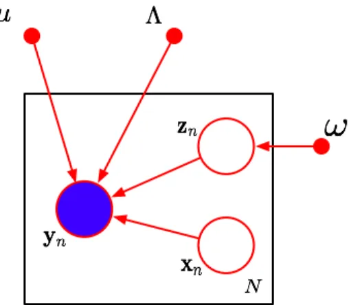
The mixture of PPCA (MPPCA) model is deﬁned by the set of distributions (15), (16) and (12). These distributions can be used to form a graphical representation, shown in ﬁgure 1.

3.2 EM algorithm for Maximum Likelihood solution

The model presented in section 3.1, and summarized in ﬁgure 1, is a latent variable model, and an EM algorithm for the estimation of its parameters {ω, µ, Λ} and la-tent variables {X, Z} can be derived [2]. The complete data log-likelihood LC =

"N

(8)

Figure 1: Directed Acyclic Graph of the MPPCA model. Circles denote random variables (respectively known and unknown for full and empty circles). Points denote parameters to be estimated.

The algorithm starts with the initialization of the model parameters. All component weights ωk are initialized to _K1, the component means µ are scattered randomly in the

data domain, and the factor matrices Λ are set with random orthogonal vectors.

The E step consists in ﬁnding the moments of the posterior distributions over latent variables X and Z given the current model parameters.

The posterior moments for Z can be interpreted as component responsibilities, and determined straightforwardly using Bayes’ rule:

E[znk = 1] = rnk ∝ p(znk = 1|ω)p(yn|znk = 1, µ, Λ) (17)

with probabilities given by equations (14), (13). These estimators are then normal-ized so that"K

k=1rnk= 1.

As reﬂected by equation (16), posterior moments for X are now conditioned on a speciﬁc component. Actually, their expressions remain very similar to (6) and (7), but are now derived for each component:

E[xn|znk = 1] = E[xnk] = M−1_k ΛTk(yn− µk) (18)

E[xnxTn|znk = 1] = E[xnkxTnk] = τ−1M−1k + E[xnk]E[xnk]T (19)

with Mk = τ−1Iq+ ΛTkΛk.

(9)

w.r.t. the model parameters: ωk= 1 N N ! n=1 rnk (20) µk= "N n=1rnk(yn− ΛkE[xnk]) "N n=1rnk (21) Λk= # N ! n=1 rnk(yn− µk)E[xnk]T $# N ! n=1 rnkE[xnkxTnk] $−1 (22)

Again, E and M steps are iterated until convergence of LC. Local maxima for

component-speciﬁc scaled principal subspace bases are recovered using (5). The EM algorithm presented in this section was reported for self-containment; if desirable, details may be found in [2].

4 Extension of the variational method to handle a MPPCA

model

4.1 Motivation

The subspace dimensionality of a PCA transform is usually determined empirically, for example by using an 80% threshold for the captured variance:

q_threshold = arg min

q & ' q ! i=1 λq ( >80% ) (23)

Minka [16] proposed an alternative Bayesian criterion for the automatic estimation of q for a given PPCA model. The Laplace method is used in order to derive an asymp-totical approximation to the posterior probability of q. Efficiency is achieved through the availability of the criterion in closed form, depending only on the set of eigenvalues. This can be seen as a rigorous alternative to the usual empirical procedure.

The algorithm presented in section 3.2 relies on the explicit knowledge of the num-ber of components K and the numnum-ber of factors per component qk. This information is

generally unknown by advance: but having deﬁned a probabilistic formulation provides us with tools for the inference of these values. As for the single PPCA case, Bayesian methods may be employed for this purpose.

The classical solution is to train models of various complexities (i.e. varying K and qk), and use selection criteria and validation data sets to compare these models. For

example, BIC [17], AIC, or other criteria more adapted to the mixture model case [18] may be employed. However, this approach requires multiple trainings before selecting the adequate model structure, which might be prohibitive under some system designs.

(10)

In this section, we rather propose to adapt the variational Bayesian framework to the MPPCA model. This general purpose technique, speciﬁcally designed for rigorous approximation of posterior probability models, was proposed in [19, 20], and reviewed in [21, 22]. It was successfully applied to the Gaussian Mixture Model (GMM) case [19, 20, 21], the PPCA case [13], or to the mixture of factor analyzers case [14, 15]. To our knowledge, it has not been applied to the MPPCA case yet. Mixture of factor ana-lyzers and MPPCA models are related, yet differ by the employed noise model (diagonal for factor analyzers, isotropic for PPCA). Also, the set of sufficient statistics in appendix A is an algorithmic improvement introduced in this paper.

In the remainder of this section, we extend the probabilistic model from section 3, in order to apply the variational Bayesian framework. Then, we put forward a EM-like algorithm for a local optimization of the MPPCA model.

4.2 Probabilistic model

The model exposed in section 3.1 is extended, with parameters modeled as random vari-ables rather than as point estimates. From the variational point of view, all parameters and latent variables are random variables, for which we want to determine posterior distributions.

with Dir() and Ga() respectively the Dirichlet and gamma distributions, and hyper-parameters subscripted by 0. This model for the hyper-parameters may be interpreted as a prior, i.e. some clue about the range of values that the real parameters may take. The objective is then to infer a posterior for these parameters, which is practically a compro-mise between prior information and evidence from data. The full model is summarized

(11)

under a graphical form in ﬁgure 2.

Figure 2: Directed Acyclic Graph of the MPPCA model, with all data and parameters modeled by random variables.

In this model, hyper-parameters shape the priors, and are statically set with unin-formative values. As the number of output components may be potentially high, K is set to some high value, and α0 is set to a low value reﬂecting our preference towards

simple models; indeed, for α0<1, the modes of the Dirichlet distribution nullify at least

one of the ωk. a0 and b0 are set to small values, and a0= b0, so as to assign equal prior

roles to all columns in factor matrices. These serve as prior information for {νkj}, which

are precision parameters for the columns of the factor matrices. This model setting is inspired by the Automatic Relevance Determination [23]; in brief, maximizing the likeli-hood of data under this model conducts some of the νkj to high values. The associated

factor columns then tend to be void, leaving only the effective ones with low νkj values.

µ0k are scattered in the data domain.

Let us remark that the priors over ω and Λ are the keys to Bayesian automatic complexity determination. In other words, a posterior of the model presented in this section would naturally have the appropriate number K" _{< K} _{of non-zero ω}

k posterior

moments, and for each associated factor matrix, the appropriate number q"_k < q_k of columns with a posterior νkj set to a low value. Thus qk may be all set to q = d − 1,

(12)

4.3 The Variational Bayesian EM algorithm for the MPPCA

As an EM-like approach, the variational method starts with the formulation of the complete likelihood:

p(Y, X, Z, ω, µ, Λ, ν|α0, a0, b0, µ0, ν0) (28)

= p(Z|ω)p(Y|Z, X, Λ, µ)p(X|Z). p(ω|α0)p(Λ|ν)p(ν|a0, b0)p(µ|ν0)

Hyper-parameters are only used as a static parameterization, and may be omitted in this expression. Thus the complete log-likelihood may be written:

LC = ln p(Y, X, Z, ω, µ, Λ, ν) (29)

The true posterior p(X, Z, ω, µ, Λ, ν|Y) that maximizes LC requires intractable

inte-grations. Therefore, there exists no systematic way to obtain it, and its functional form is undetermined. The purpose of the variational approach is to ﬁnd an approximation to this true posterior within a simpler and well-deﬁned family of distributions, so that the tractability is guaranteed.

A variational distribution set is deﬁned, and factorizes exactly as does the prior distribution in the model:

q(X, Z, ω, µ, Λ, ν) = q(X, Z)q(ω, µ, Λ, ν) (30) q(X, Z) = N % n=1 q(xn|zn)q(zn) q(ω, µ, Λ, ν) = q(ω) K % k=1 q(µk)q(Λk|νk)q(νk)

Let us remark that these variational distributions have the same functional form as their respective prior. Then, the following theorem holds [22] :

Theorem 4.1 Let θ = {θ1, . . . , θm} be any factorized parameter and latent variables

set, and Y an observed data set. The approximate distribution verifying:

q∗(θ) = arg min q(θ) KL*q(θ)||p(θ|Y)+ (31) is obtained when: q∗(θi) ∝ exp ' Eq∗_(θ /i)[LC] ( , i= 1, . . . , q (32) or equivalently, (33) ln q∗(θi) = Eq∗_(θ /i)[LC] + const, i = 1, . . . , q (34)

(13)

with KL(.||.) the KL divergence between two probability distributions, and θ_/i the set {θj} in θ for which j &= i,

and q∗_(θ

/i) =,mj=1,j$=iq∗(θj)

This theorem provides us with a systematical way to obtain an approximation q∗_{(X, Z, ω, µ, Λ, ν)}

to the true and unknown posterior. The algorithm starts with the initialization of m − 1 elements of q∗_{(), e.g. with their respective prior. The m-th element is updated using}

theorem 4.1, followed by the successive updates of the m − 1 ﬁrst elements. Each such step (i.e. succession of m updates) was proven to increase the expected value for LC [21].

This property led to the EM-like denomination. Variational updates are performed until convergence. In other words, an estimate for the optimal q∗_{() is progressively reﬁned.}

Let us remark that E[LC] can be viewed as a lower bound to a constant, marginalized

likelihood (i.e. integrated over all unknowns) [21]. Thus it can be computed and used to detect the convergence of the variational algorithm.

Similarly to EM, this scheme performs a local optimization. But variational EM algorithms perform a functional optimization, as opposed to point-wise for EM. Thus, some regularity is guaranteed for the solutions, and usual degeneracies of EM schemes for mixture models are avoided [24, 21].

Using expression (29) for all the terms in LC, and theorem 4.1, we obtain the

for-mulas for the update of the variational distributions, given in appendix A. Let us note that variational distributions can be characterized either by their ﬁrst and second order moments (e.g. E[xnk] or E[Λij_k

2

]), or their shaping hyper-parameters (e.g. αk, bkj). All

are deduced by the usage of theorem 4.1.

In appendix A, we regrouped updates for the variational distributions over latent variables in the E step. Sufficient statistics are accumulators that are built using the current estimations for latent variables. Variational distributions over model parameters are updated using these accumulators. Updates for model parameters are regrouped in an M step, by analogy to the classic EM formulation. Practically, the algorithm starts with the initialization of the variational distributions over parameters (i.e. q(ω, µ, Λ, ν)) with their respective prior, and proceeds with the E step.

Convergence may be assessed by monitoring the value of Eq∗[L_C]. The obtained

estimates for Λk are post-processed using (5).

The algorithm outputs a posterior MPPCA:

output MPPCA = {ωk, µk,Λk, τ|αk > α0} (35)

The variational Bayesian algorithm for the mixture of PPCA will be further iden-tiﬁed by VBMPPCA. An analogous application of theorem 4.1 to the GMM case was

(14)

already proposed in the literature [21]. The associated algorithm will be further known as VBGMM.

As proposed in section 4.2, the algorithm can be run with factor matrices of the maximal possible size, i.e. q = d − 1 columns, or less if computational time is an issue, at the risk of some information loss in the posterior. In the same section, we argued that the model ensures dimensionality reduction with precision parameters over the columns of the factor matrices. After post-processing, factor matrices are ordered by decreasing magnitude (see section 2.1): so a systematic way to infer the proper dimensionality speciﬁc to each output component can be proposed:

Data: An output MPPCA

Result: output MPPCA with dimensionality reduced factor matrices for each component k in the model do

1

currentDivergence← +∞ ;

2

curQ← 0 ;

3

while currentDivergence > threshold do

4

curQ← curQ + 1 ;

5

Λtemp← ﬁrst curQ columns of Λk ; 6 currentDivergence← 7 KL ' N (0, ΛkΛTk + τ−1Id)||N (0, ΛtempΛTtemp+ τ−1Id) ( ; end 8 Λk ← ﬁrst (curQ − 1) columns of Λk ; 9 end 10

Algorithm 1: Inference of dimensionality for output factor matrices

The KL divergence between two Gaussians is deﬁned in closed form. The algorithm 1 tries to form the covariance of the marginal for data Y with a limited number of factors, and stops when the last added factor did not change signiﬁcantly the shape of the distribution. This means that factors columns with index greater or equal to curQare close to void, and can be pruned from output factor matrices. Subspaces with reduced dimensionality are thus built.

5 Aggregating mixtures of PPCA

A straightforward way of aggregating MPPCA models separately estimated on different data sources is to add them. However if sources reflect the same underlying generative process, the resulting mixture is generally unnecessarily complex, i.e. redundant, with regard to a model estimated on the union of the data sets. In this section, we show first how the addition of input MPPCA models can be seen as the limit representation of a virtual data set [1]. This representation is then inserted into the model described in section 3, as a substitution for an ordinary data set. The associated variational EM algorithm is supplied. It outputs the low complexity model that best fits the data which

(15)

would have been generated from the redundant input mixture, without relying either on the data itself or on any sampling scheme.

5.1 Model

A full sample (i.e. data and indicator variables, all observed) originating from an arbi-trary and known redundant MPPCA with L components may be denoted by (Y, Z") = {yn,z"n}. Let us regroup elements from this sample according to the values taken by z"n,

and deﬁne ˆyl= {yn|z_nl" = 1}, and ˆz"_l= {z"n|z"nl= 1}.

We propose to formulate the likelihood of this sample under an unknown MPPCA model. This last model will be further known as the target, as opposed to the input model, that originated Y. To prevent ambiguities, components from the input and output models will be indexed respectively by l ∈ {1, . . . , L} and k ∈ {1, . . . , K}.

The (known) indicator variables of the sample according to the input model are collectively denoted by Z"_{: this notation is not to be confused with Z, the (unknown)}

indicator variables of this same sample according to the output model. In order to keep notations concise, and without loss of generality, we now assume that all components in the input model have factor matrices with the same number of columns, q.

The output model should not be more complex than the input model, so the same q may be used to parameterize the size of factor matrices in the output model. Let us write the likelihood of the full sample under the output MPPCA model:

where we used expressions (11) and (12). ω, µ and Λ collectively denote the out-put model parameters. Latent variable X is intentionally left implicit. We assumed that membership variables for all yi in ˆyl are identical, and equal to zl. This

hypoth-esis is generally acceptable, mixture models aggregation being often about combining components. Let us notice that:

|ˆz"_l| = |ˆyl| + N ωl (39)

with N the cardinal of the sample considered above. Using this approximation in (38) replaces the input data by its abstraction (i.e. sample size and input model parameters). Let us rewrite (37) as follows:

(16)

p(Y|Z, θ) = K % k=1 L % l=1 (N (ˆyl|µk,Ck))zlk = K % k=1 L % l=1 pzlk lk (40)

Deﬁning Llk= ln plkfor a speciﬁc term in (40), expanding ˆyl, and using

approxima-tion (39) gives: Llk + N ωl ! j=1 ln N (ylj|ωk, µk,Ck) (41) + N ωl # −KL-N (µl,Cl)||N (µk,Ck). − H-N (µl,Cl) . $ (42)

where we used the law of large numbers to approximate the KL divergence and the entropy by a ﬁnite sum. As a consequence, N should be sufficiently large for expressions (39) and (42) to be roughly valid.

Let us underline that the likelihood (i.e. (37) and (38)) has been transformed so that it depends on the input sample only through the input model parameters. N can then be chosen arbitrarily. In other words, we use a virtual sample, but only process input model parameters. This idea was initially formulated in [25, 26] for Gaussian mixtures. This approximation signiﬁcantly reduces the complexity of the problem, as it now only depends on the size of the input mixture L.

The KL divergence between Gaussians and the entropy of a Gaussian both have closed form expressions. Using these to expand (42) gives:

Llk= N ωl # −d 2ln(2π) − 1 2ln det(ΛkΛ T k + τ−1Id) −1 2Tr-(ΛkΛ T k + τ−1Id)−1[ΛlΛTl + τ−1Id + (µl− µk)(µl− µk)T] . $ (43)

τ is generally a low value, and its inﬂuence is discarded in the rest of the section. As ΛlΛTl = "q j=1Λ .j l Λ .j l T

, plk can be approximated by the combined likelihoods of the

input means and factor columns. Thus after renormalization:

plk=  N (µ_l|µ_k,C_k) q % j=1 N (Λ.j_l |0, Ck)   N ωl (44)

Using (44) with (40) and (38), an approximation to the input sample likelihood is obtained:

(17)

p(Y, Z|ω, µ, Λ) = L % l=1 K % k=1 3 ωN ωl k 4 N (µl|µk,Ck) . q % j=1 N (Λ.j_l |0, Ck) 5N ωl6zlk (45)

In (45), all terms are members of the exponential family. Such a probability distri-bution, taken to any power and normalized, is still a member of the exponential family: thus N ωl can be incorporated into the model parameters, giving:

p(Y, Z|ω, µ, Λ) = p(Z|ω)p({µl,Λl}|Z, µ, Λ) (46) where we deﬁned: p(Z|ω) = L % l=1 K % k=1 -ωN ωl k .zlk ₍₄₇₎ p({µl,Λl}|Z, µ, Λ) = L % l=1 K % k=1 ' N (µl|µk,(N ωl)−1Ck) . q % j=1 N (Λ.j_l |0, (N ωl)−1Ck) (zlk (48)

Let us note that on the left hand side of (46), Y still appears, while on the right hand side, only input model parameters are used. This convention was chosen for homogeneity to the model presented in section 4.2. Notice that the marginal for the virtual sample p(Y|ω, µ, Λ), that would be obtained using (46), is a mixture of products of Gaussians.

All Gaussian terms in (46) still depend on Ck, and, using theorem 2.1, can be

extended with x latent variables. As each component of the mixture is made of the product of 1 + q terms, the size of X is increased accordingly. To prevent any ambiguity, let us deﬁne X = (X1,X2), X1 = {x1l} and X2 = {x2lj|j ∈ 1 . . . q}. The likelihood of

the complete data can then be written as:

p(Y, X, Z|ω, µ, Λ) = p(Z|ω)p({µl,Λl}|Z, X1,X2, µ,Λ)p(X1,X2|Z) (49) with p({µl,Λl}|Z, X1,X2, µ,Λ) = L % l=1 K % k=1 ' N-µ_l|Λkx1l+ µk,(N ωlτ)−1Id . q % j=1 N-Λ.j_l |Λkx2lj,(N ωlτ)−1Id . (z_lk and p(X1,X2|Z) = L % l=1 K % k=1 ' N-x1l|(N ωl)−1Iq . q % j=1 N-x2lj|(N ωl)−1Iq . (zlk

(18)

5.2 Variational EM algorithm

In the previous section, we showed how the likelihood of a virtual sample may be ex-pressed in terms of the sole parameters of a redundant input MPPCA model, without any actual sampling scheme. Thus by substituting (49) to the terms p(Z|ω)p(Y|Z, X, Λ, µ)p(X|Z) in (28), we obtain:

p(Y, X, Z, ω, µ, Λ, ν) = p(Z|ω)p({µl,Λl}|Z, X1,X2, µ,Λ)

.p(X1,X2|Z)p(ω|α0)p(Λ|ν)p(ν|a0, b0)p(µ|ν0) (50)

The variational Bayesian algorithm described in section 4.3 can then be extended straightforwardly. The associated variational distribution follows the factorization sug-gested by (50), and uses the same functional forms for its terms:

q(X1,X2,Z, ω, µ, Λ, ν) = q(X1,X2,Z)q(ω, µ, Λ, ν) (51) q(X1,X2,Z) = L % l=1 ' q(zl)q(x1l|zl) q % j=1 q(x2lj|zl) ( q(ω, µ, Λ, ν) = q(ω) K % k=1 q(µk)q(Λk|νk)q(νk)

Using theorem 4.1 with (50) and (51), EM re-estimation equations can be obtained. These are given in appendix B. These update expressions are used exactly as already suggested in section 4.3, until convergence of the modiﬁed expected value for LC (i.e.

the log of expression (29)). This new variational algorithm will be further known as VBMPPCA-A. The variational algorithm for the aggregation of GMM components, al-ready proposed in [11], is denoted as VBGMM-A, and will be used for comparison in section 6.

Let us consider a single component from the output model. As stated earlier, after convergence, its column vectors are ordered by decreasing magnitude. Let us notice that each dimension of a latent variable x ∈ X can be interpreted as a coefficient for a linear combination of these column vectors. It seems natural to combine first columns of input factor matrices to form the first column of a component’s output factor matrix, and so on. Therefore, during the first E step of the algorithm, instead of performing the update for x2lj variables, these are initialized with canonical vectors:

x2lj = ej (52)

In the subsequent E steps, the moments for these variables may be updated as usual. Updating (1 + q) x variables instead of a single one burdens our E step. But this loss is not critical, as our algorithm now scales with a number of input components, instead of

(19)

a number of data elements.

Moreover, experimentally VBMPPCA-A happened to perform better with no update of X2. The results presented in this paper used this implementation.

At the beginning of section 5.1, we assumed the same parameter q for all input components. Let us consider the case where this should not be true: then ql is the factor

matrix size associated with input component l. We set qmax= max ql. Then, appending

qmax− qlvoid columns to each input factor matrix, and statically setting associated x2lj

to 0 is equivalent to using the same q for all components.

6 Experimental results

We ﬁrst apply VBGMM and VBMPPC to synthetic data sets that illustrate various prototypical situations1_{, and discuss their relative performances. We then report results}

on the same data set, pertaining to the model aggregation task, ﬁrst comparing GMM and MPPCA models, then sequentially aggregating MPPCA models. Finally, similar experiments are reported, on two well-known real data sets.

6.1 Model fitting task : comparison of VBGMM and VBMPPCA

First we propose a thorough comparison of VBGMM and VBMPPCA methods. For this purpose, we designed the 3 following data generating processes:

• SYN1: this process samples data elements from 4 well-separated 2D Gaussian components, and linearly transforms them with additive noise to form a data set with d = 9. An example for the original 2D signal is provided on ﬁgure 3.

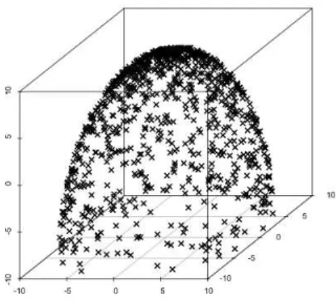
• SYN2: this process generates elements along a semi-sphere. It is exempliﬁed on ﬁgure 4.

• SYN3: this process samples elements along a 2D circle with additive noise. As for SYN1, this original signal is transformed to 9D, with additional noise, using a linear transform. An example of the 2D process is shown on ﬁgure 5.

The linear transforms used to generate samples from SYN1 and SYN3 are designed to produce artiﬁcial linearly redundant information. Thus a method like PCA should recognize the original signal in this context. SYN2 is characterized by a 2D manifold within a 3D space, which dimensionality reduction methods should also be able to recog-nize. Employed dimensionalities (up to 9 in our 3 examples) may seem modest, but were chosen for their clear identiﬁability and for tractability of VBGMM (which is O(d3_)).

1_{Our open-source implementation in R (optimized and documented) for estimating the models and}

(20)

Figure 3: Sample from SYN1 Figure 4: Sample from SYN2

Figure 5: Sample from SYN3

These three processes were used to generate training data sets of various sizes, from 50 to 1000 elements. 10 testing sets of 1000 elements were also generated for validation purpose.

100 training sets were generated for each size, and each was used to estimate a model, either with VBGMM or VBMPPCA. VBMPPCA was parameterized with the maximal potential rank for each component, i.e. q = d−1. The quality of each model was assessed using the following characteristics:

• The effective rank of the component subspaces. • The effective number of components K"_.

• The average log-likelihoods of the validation data sets. In order to perform this operation, MPPCA models are transformed to GMM using the identity Ck =

τ−1Id+ ΛkΛTk. In the speciﬁc case of SYN1 and SYN3, only the 2 relevant

(21)

These measures were averaged over the training and testing sets, and are reported in tables 1, 2 and 3. Each measure is associated to its standard deviation (bracketed in the tables).

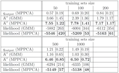
training sets size

50 100 200 qoutput (MPPCA) 0.59 [0.29] 0.85 [0.31] 1.13 [0.31] K" (GMM) 3.95 [0.36] 3.84 [0.37] 3.84 [0.37] K" (MPPCA) 5.25 [1.19] 5.37 [1.23] 4.78 [0.91] likelihood (GMM) -4709 [307] -4527 [104] -4415 [117] likelihood (MPPCA) -4742 [828] -4417 [43] -4380 [17]

training sets size 500 1000 qoutput (MPPCA) 1.51 [0.21] 1.66 [0.16] K" (GMM) 3.93 [0.26] 3.95 [0.22] K" (MPPCA) 4.15 [0.52] 4.03 [0.36] likelihood (GMM) -4290 [79] -4239 [91] likelihood (MPPCA) -4379 [48] -4373 [27]

Table 1: Comparisons between VBGMM and VBMPPCA, SYN1 process. Best results are bold-faced.

From table 2, we clearly see that the MPPCA model is not suited to a process such as SYN2. Data sampled from SYN2 lies on a manifold, but is not associated to clear clusters, which mixture ﬁtting algorithms try to discover (see ﬁgure 6). Moreover, the more dimensions the problem has, the better PPCA performs. On the contrary, in ex-treme cases (such as principal components of a 3D space, or sparse data), it is almost equivalent to model data with a linear transformation of a 1D variable with added noise, or with pure noise. This ambiguity drives VBMPPCA into bad local maxima.

With higher dimensions and more plentiful data, manifold learning by VBMPPCA can be much more accurate (see table 3 with semi-circle data, and ﬁgure 7 for a visual example). The case of cluster-shaped data with redundant dimensions, such as simulated by SYN1, is also correctly handled, as table 1 shows similar performance of VBGMM and VBMPPCA on this data set.

6.2 Model aggregation task : comparison of VBGMM-A and

VBMPPCA-A

The models that were estimated in section 6.1 are then used as pools of input models for aggregations with VBGMM-A and VBMPPCA-A algorithms. More speciﬁcally, a separate pool is formed with models from each training set size. Pools associated with training set sizes 100 and 1000 are retained in this section.

(22)

training sets size 50 100 200 qoutput (MPPCA) 0.13 [0.14] 0.15 [0.08] 0.20 [0.10] K" (GMM) 7.01 [1.31] 9.25 [1.23] 10.9 [1.26] K" (MPPCA) 8.75 [1.88] 17.63 [2.51] 25.97 [4.49] likelihood (GMM) -9321 [583] -8352 [109] -7981 [60] likelihood (MPPCA) -19882 [4357] -11202 [1008] -8964 [279]

training sets size

500 1000 qoutput (MPPCA) 0.52 [0.25] 1.22 [0.36] K" (GMM) 13.84 [1.27] 16.83 [1.44] K" (MPPCA) 18.72 [7.22] 8.44 [2.70] likelihood (GMM) -7581 [29] -7321 [20] likelihood (MPPCA) -8352 [151] -8269 [131]

Each experiment is conducted with varying amounts of input models selected ran-domly in their pool. 10 runs are performed for each possible conﬁguration (i.e. a speciﬁc training set size and amount of input models to aggregate). For a fair comparison, only input MPPCA models are used: the same selected inputs are used with VBMPPCA-A, and simply converted to GMM models before using VBGMM-A.

MPPCA model ﬁtting was shown to be irrelevant with SYN2 in section 6.1. Thus SYN1 and SYN3 processes were solely considered in this section. In tables 4 and 5, av-eraged quality measures and their standard deviations are indicated. The log-likelihood values are estimated using the validation data sets presented in section 6.1.

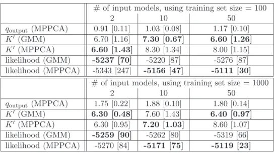
VBMPPCA-A performs slightly better than VBGMM-A (see tables 4 and 5). As in the previous section, the rank associated to component subspaces tends to be better recovered when using larger training data sets. Models estimated with VBMPPCA-A are associated to better likelihoods, at the expense of some model complexity (i.e. K" tends to be higher with VBMPPCA-A). Besides, VBMPPCA-A behaves well as a larger number of input models are aggregated. This may originate from the inﬂuence of the component-wise factor matrix combination (see section 5.2).

Let us note that while VBMPPCA used q = d − 1, VBMPPCA-A is parameterized according to its input components (see end of section 5.2). Each of these have qoutput<

d− 1 set as a posterior w.r.t. to their respective training set. Thus generally q < d − 1 when using VBMPPCA-A. As the complexity of the latter is O(q3), its computational

(23)

training sets size 50 100 200 qoutput (MPPCA) 0.57 [0.19] 0.69 [0.20] 0.84 [0.21] K" (GMM) 3.66 [1.45] 2.39 [1.36] 1.79 [1.17] K" (MPPCA) 7.55 [1.22] 7.78 [1.41] 7.17 [1.17] likelihood (GMM) -5882 [263] -6004 [344] -6112 [354] likelihood (MPPCA) -5546 [420] -5209 [53] -5163 [61]

training sets size 500 1000 qoutput (MPPCA) 1.21 [0.22] 1.49 [0.19] K" (GMM) 1.16 [0.65] 1.03 [0.30] K" (MPPCA) 6.46 [0.85] 6.50 [0.72] likelihood (GMM) -6294 [214] -6335 [106] likelihood (MPPCA) -5149 [57] -5138 [48]

cost is much lower that VBGMM-A performed over the same inputs, with comparable results.

6.3 Model aggregation task : incremental aggregation of MPPCA

models

In section 6.2, the input models, i.e. the selection we mean to aggregate in an experiment, are all available at once. In some distributed computing settings, such as gossip, models may become available incrementally, as their production and broadcast over a network progresses. Thus we may consider the possibility to update a reference model (see ﬁgure 8).

Let us consider again the input model collection of section 6.2. Speciﬁcally, we use the sub-collection associated with training sets of 1000 elements, for SYN1 and SYN3 processes. We propose to simulate an incremental aggregation, by updating a reference MPPCA model successively with all 100 input models available for each process. The quality of the model eventually obtained is then assessed. This experiment is performed 10 times. Averaged measures and standard deviations associated with these runs are reported in table 6.

Results shown in table 6 indicate that the usage of VBMPPCA-A in an incremental setting challenges the standard described in section 6.2 (i.e. reported in tables 4 and 5), either regarding to the number of components or the likelihood of the estimated models.

(24)

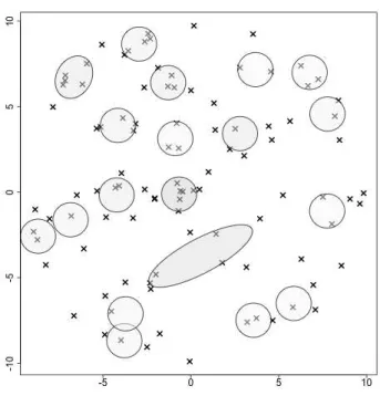
Figure 6: A set from SYN2 process (projected on 2 dimensions), used to train a MPPCA model.

6.4 Experiments on real data sets

The algorithms presented in this paper are also evaluated on the following two real data sets:

• Pen-based recognition of handwritten digits data set (further denoted as pen) [27]: this data set was built with measurements of digit drawings on a tablet. Its 10992 elements are described by 16 numeric attributes. These are pretty naturally gath-ered in 10 classes (i.e. one for each digit).

• MNIST database of handwritten digits (further denoted as hand) [28]: the training set of this database (60000 elements) was used for these experiments. Each element is described by a 28x28 image patch of a specific digit (see figure 9); these can be viewed as numeric 784-dimensional vectors of pixel intensities. As for the pen data set, the classes are naturally defined as the digit contained in each image patch. First, training and testing sets are delimited within these data sets:

• The 5000 ﬁrst elements constitute the training set for pen. The complementary set is used for validation.

• 10000 elements are randomly selected in hand to form the validation set. The complementary set of 50000 elements is used for training.

(25)

Figure 7: GMM (left) and MPPCA (right) trained with a data set from SYN3.

Similarly to the experiments on synthetic data, the training data sets are further divided in subsets (25 subsets of 200 elements for pen, 50 subsets of 1000 elements for

hand). Models are estimated on these subsets using either VBGMM or VBMPPCA.

Measures and comparisons are provided in table 7 for models estimated on subsets of pen and hand. As VBGMM and GMM likelihood computation are intractable on 784-dimensional data sets, measurements are reported only for VBMPPCA. To limit the computational load with VBMPPCA, the explicit constraint q < 9 is used for both data sets. Let us note that this ability of handling intractable mixture problems is an advantage of the MPPCA model over the GMM, as underlined in the introduction.

Estimating a mixture model on a data set can be interpreted as a clustering task. Thus the validation subsets, and their associated true labels, are used to compute the clustering error of each output model. Let us note that pen and hand data sets are traditionally used in a supervised learning setting [28, 3]. Yet it seemed interesting to see how an unsupervised approach would perform comparatively. We use the error function proposed in [29, 30]. This function is specially adapted to the clustering task because it measures how two label sets are related, and is still meaningful if ground truth and inferred numbers of clusters and semantics differ.

VBMPPCA leads to more complex models for pen data set. This may be due to the constraint imposed on q. However, measured clustering errors indicate sensible estima-tions. Let us note that the output subspace ranks for components reﬂect the underlying complexity of each data set: only 2.76 dimensions are used in average among the 8 pos-sible for pen, while almost all are used for hand.

The clustering performance of VBMPPCA is also illustrated with confusion matrices, in ﬁgure 10 for pen, and ﬁgure 11 for hand. These matrices are estimated by the average

(26)

# of input models, using training set size = 100 2 10 50 qoutput (MPPCA) 1.11 [0.19] 1.03 [0.16] 1.18 [0.14] K" (GMM) 4.90 [0.99] 4.30 [0.48] 4.30 [0.68] K" (MPPCA) 4.50 [0.97] 6.30 [1.25] 7.80 [1.23] likelihood (GMM) -4391 [52] -4356 [8] -4425 [216] likelihood (MPPCA) -4425 [186] -4334 [6] -4325 [3]

# of input models, using training set size = 1000

Table 4: Comparisons between VBGMM-A and VBMPPCA-A, SYN1 process. Best results are bold-faced.

of 10 experiments on training subsets. The difference between the ground truth and inferred number of clusters was handled by selecting the 10 most populous clusters of each estimated model. The selected clusters were then labeled according to the most frequent ground truth in their associated elements.

In ﬁgure 10, we see that 10 estimated clusters are roughly sufficient to explain pen data. 0’s and 1’s are well recognized, but we see that some digits are often mistaken, e.g. 7 is interpreted as 6 or 2, and 6 is often interpreted as 5. For the latter case, the similar shape explains the confusion.

Examination of ﬁgure 11 clearly shows that 10 clusters are not sufficient to explain

hand data. Lots of small clusters that were left out (see computed values for K in table

7, largely greater than 10) as required by the confusion matrix representation. These would greatly help reduce the classiﬁcation error observed in ﬁgure 11. Yet, we can underline some interesting facts: pixel data also leads to an easy recognition of 0’s and 1’s, while digits from 5 to 9 are difficult to cluster clearly.

In figure 12, we show some examples of means for MPPCA models estimated on subsets of hand. A label is estimated for each component using the validation data set, by using a majority vote. The first 4 factors of a component are also presented as an example. Lighter or darker gray values indicate where the influence of this factor is located in the image space. We see how each factor embodies different variations of elements in its associated component.

Aggregations are then performed using all these input models. Results, when avail-able, are presented in table 8. As in section 6.2, MPPCA input models are used with both VBMPPCA-A and VBGMM-A. Conversions are performed when appropriate.

(27)

# of input models, using training set size = 100 2 10 50 qoutput (MPPCA) 0.91 [0.11] 1.03 [0.08] 1.17 [0.10] K" (GMM) 6.70 [1.16] 7.30 [0.67] 6.60 [1.26] K" (MPPCA) 6.60 [1.43] 8.30 [1.34] 8.00 [1.15] likelihood (GMM) -5237 [70] -5220 [87] -5276 [87] likelihood (MPPCA) -5343 [247] -5156 [47] -5111 [30]

# of input models, using training set size = 1000

Table 5: Comparisons between VBGMM-A and VBMPPCA-A, SYN3 process. Best results are bold-faced.

SYN1 SYN3 qoutput 1.76 [0.02] 1.75 [0.13]

K" 4.10 [0.32] 7.10 [0.99] likelihood -4379 [46] -5240 [45]

Table 6: Results of incremental aggregations with SYN1 and SYN3 processes.

Clustering errors for aggregated MPPCA models tend to be much lower (i.e. better performance) than what is obtained for GMM aggregation, with similar model com-plexities. Compared to baseline MPPCA estimation (see table 7), aggregation causes a slight loss in classiﬁcation error, associated with a much lower model complexity. Thus MPPCA aggregations produce good summaries of the input models.

7 Discussion about the MPPCA model

In VBMPPCA and VBMPPCA-A algorithms, the moments of variational distributions are strongly coupled (see equations (53), (54), (55), (56) and (57)). This may cause biases, or, from a computational point of view, decreases of the lower bound value as-sociated with VBMPPCA and VBMPPCA-A algorithms (see section 4.3). Practically, after a sufficient number of iterations, this bias eventually disappears; but this compro-mises the usage of the lower bound as a reliable convergence criterion. Instead, measures of the agitation of Z may be used [15].

(28)

Figure 8: Incremental aggregation in the context of local models broadcasted on a network pen hand qoutput (MPPCA) 2.76 [0.27] 7.17 [0.29] K" (GMM) 12.7 [1.8] K" (MPPCA) 24.2 [3.0] 34.8 [6.1] error (%, GMM) 12.6 [3.0] error (%, MPPCA) 9.0 [1.5] 10.8 [1.2]

Table 7: Results for VBGMM and VBMPPCA on pen and hand data sets

8 Conclusion and perspectives

In this paper we proposed a new technique that performs the estimation of MPPCA models, and their aggregation. A fully probabilistic and Bayesian framework, along with the possibility to deal with high dimensional data motivated our approach. Theoretical justiﬁcations were developed, and some illustrative results were detailed. Advantages and limitations of the proposed approach were highlighted.

Results obtained in section 6 show that processing over subspaces and principal axes provide an interesting guideline to carry out aggregations. Components are ﬁtted ac-cording to their intrinsic subspace dimensionality, instead of a crisp covariance structure combination. Furthermore, properties of ML PPCA solutions (and particularly the abil-ity to recover easily the ordered principal axes set), provide us with some strong prior knowledge, and a well-deﬁned initialization scheme.

(29)

Figure 9: Sample image patch from the hand data set pen hand qoutput (MPPCA) 3.27 [0.31] 7.12 [0.37] K" (GMM) 13.2 [1.7] K" (MPPCA) 13.0 [1.9] 27.5 [6.3] error (%, GMM) 16.9 [3.2] error (%, MPPCA) 11.2 [1.4] 11.7 [1.9]

Table 8: Results for VBGMM-A and VBMPPCA-A on pen and hand data sets

we believe there should be some interesting derivation of the mixture of PPCA in the domain of semi-supervised clustering. Let us suppose, as formalized and used in [31], that we have a set of ”must-link” constraints (i.e. pairs of data items that should be clustered together), and ”must-not-link” constraints (i.e. data that should not be in the same group). Under the hypothesis of compact clusters (i.e. each cluster should lie on a compact and approximately linear manifold, see [32] for discussion), we may implement these as follows :

• must-link : for now, each factor matrix is initialized with a random orthogonal matrix (e.g. see section 3.2). Data items we believe to be in the same component may be used to influence this initialization, and guide the algorithm towards a specific local minimum (as we said earlier, real world data might be strongly non Gaussian, so there might be several posterior models with similar likelihoods but significant pairwise KL divergences).

• must-not-link : As we employed a Bayesian integration scheme, this kind of con-straint might be modeled by some pdf (e.g. as in [33]). This remark is not speciﬁc to the MPPCA model: but we might take advantage of its principal subspace structures.

(30)

Figure 10: Sample confusion matrix of MPPCA clusterings (pen data), showing the distribution of 200 data elements.

Appendices

A

EM expressions for VBMPPCA

• E step: Σx_k =-Iq+ τ E[ΛTkΛk].−1 Eq(xn|znk=1)[xn] = E[xnk] = τ ΣxkE[Λ T k](yn− E[µk]) Eq(xn|znk=1)[xnx T

n] = E[xnkxTnk] = Σx_k+ E[xnk]E[xnk]T

rnk ∝ exp 7 ψ(αk) − ψ ' K ! j=1 αj ( −1 2Tr(E[xnkx T nk]) −τ 2 #

,yn,2+ E[,µk,2] − 2(yn− E[µk])TE[Λk]E[xnk]

− 2yT_nE[µk] + Tr(E[ΛTkΛk]E[xnkxTnk])

$8

(31)

Figure 11: Sample confusion matrix of MPPCA clusterings (hand data), showing the distribution of 1000 data elements.

• Sufficient statistics: Nk= N ! n=1 rnk y2k= N ! n=1 rnk||yn||2 yk= N ! n=1 rnkyn sk= N ! n=1 rnkE[xnk] sy_k= N ! n=1 r_nkynE[xnk]T Sk= N ! n=1 r_nk_E[x_nkxT_nk] (54) • M step: αk= α0k+ Nk akj = a0+ d 2 bkj = b0+ 1 2 d ! i=1 E[Λijk 2 ] ΣΛk = (diag(E[νk]) + τ Sk) −1 E[Λijk 2 ] = E[Λi.kΛi.k T ]jj Σµk = # ν0+ τ Nk $−1 Id (55)

(32)

Figure 12: Mean and factor examples of MPPCA models on the hand data set. E[ΛTkΛk] = d ! i=1 E[Λi.kΛi.k T ] E[Λi.k] = ΣΛkτ # syi._k− E[µik]sk $ E[µk] = Σµk # ν0µ0k+ τ (yk− E[Λk]sk) $

(33)

B

EM expressions for VBMPPCA-A

• E step: Σx_kl =-N ωl[Iq+ τ E[ΛTkΛk]] .−1 = (N ωl)−1Σx_k E[x1lk] = τ N ωlΣx_klE[ΛT_k] ' µ_l− E[µk] ( = τ ΣxkE[Λ T k] ' µl− E[µk] ( E[x2lkj] = τ N ωlΣxklE[Λ T k]Λ.jl = τ ΣxkE[Λ T k]Λ.jl rlk∝ N ωl(ψ(αk) − ψ( K ! j=1 αj)) − N ωl 2 Tr(E[x1lkx T 1lk] + q ! j=1 E[x2lkjx2lkj]) − τ N ω_l 2 9 ,µl,2+ q ! j=1 ,Λ.j_l ,2

+ E[,µk,2] − 2µTlE[µk] − 2(µl− E[µk])TE[Λk]E[x1lk]

− 2 q ! j=1 (Λ.j_l TE[Λk]E[x2lkj]) + Tr ' E[ΛTkΛk]-E[x1lkxT1lk] + q ! j=1 E[x2lkjxT2lkj] . (: (56) • Sufficient statistics: Nk = L ! l=1 N ωlrlk yk = L ! l=1 N ωlrlkµl sk= L ! l=1 N ωlrlkE[x1lk] sy_k = L ! l=1 N ωlrlk ' µlE[x1lk]T + q ! j=1 Λ.j_l E[x2lkj]T ( y2_k= L ! l=1 N ωlrlk ' ||µl||2+ q ! j=1 ||Λ.j_l ||2 ( Sk= L ! l=1 N ωlrlk ' E[x1lkxT1lk] + q ! j=1 E[x2lkjxT2lkj] ( (57)

• M step: as the output model remains identical, with dependence on the same set of sufficient statistics, update formulae (55) can be used.

(34)

References

[1] P. Bruneau, M. Gelgon, and F. Picarougne. Aggregation of probabilistic PCA mixtures with a variational-Bayes technique over parameters. In Proc. of Int. Conf.

on Pattern Recognition (ICPR’10), pages 1–4, Istambul, Turkey, Aug. 2010.

[2] M. E. Tipping and C. M. Bishop. Probabilistic principal component analysis.

Jour-nal of the Royal Statistical Society - B Series, 61(3):611–622, 1999.

[3] M. E. Tipping and C. M. Bishop. Mixtures of probabilistic principal component analyzers. Neural Computation, 11(2):443–482, 1999.

[4] D. Newman, A. Asuncion, P. Smyth, and M. Welling. Distributed algorithms for topic models. Journal of Machine Learning Research, 10:1801–1828, 2009.

[5] M. Bechchi, G. Raschia, and N. Mouaddib. Merging distributed database sum-maries. In ACM Conf. on Information and Knowledge Management (CIKM’2007), pages 419–428, Lisbon, Portugal, Aug. 2007.

[6] X. Fern, I. Davidson, and J. Dy. Multiclust 2010: Discovering, summarizing and using multiple clusterings. SIGKDD Explorations, vol 12(2):47–49, 2010.

[7] A. Strehl and J. Ghosh. Cluster ensembles - a knowledge reuse framework for combining multiple partitions. Journal of Machine Learning Research, 3:583–617, 2003.

[8] K. Watanabe, S. Akaho, and S. Omachi. Variational Bayesian mixture model on a subspace of exponential family distributions. IEEE Trans. Neural Networks, 20(11):1783–1796, 2009.

[9] D. Gu. Distributed EM algorithm for Gaussian mixtures in sensor networks. IEEE

Trans. Neural Networks, 19(7):1154–1166, 2008.

[10] B. Safarinejadian, M. Menhaj, and M. Karrari. Distributed variational Bayesian algorithms for Gaussian mixtures in sensor network. Signal Processing, 90(4):1197– 1208, 2010.

[11] P. Bruneau, M. Gelgon, and F. Picarougne. Parsimonious reduction of Gaussian mixture models with a variational-Bayes approach. Pattern Recognition, 43:850– 858, March 2010.

[12] A. P. Dempster, N. M. Laird, and D. B. Rubin. Maximum likelihood from incom-plete data via the EM algorithm. Journal of the Royal Statistical Society - B Series, B(39):1–38, 1977.

[13] C. M. Bishop. Variational principal components. Proc. Int. Conf. on Artif. Neural

(35)

[14] Z. Ghahramani and M. J. Beal. Variational inference for Bayesian mixtures of factor analysers. pages 12:449–455, 2000.

[15] M. J. Beal. Variational Algorithms for approximate inference. PhD thesis, Univer-sity of London, 2003.

[16] T. Minka. Automatic choice of dimensionality for PCA. Advances in Neural

Infor-mation Processing Systems, 13(514):598–604, 2001.

[17] G. Schwarz. Estimating the dimension of a model. The Annals of Statistics, 6:461– 464, 1978.

[18] T. Xiang and S. Gong. Model selection for unsupervised learning of visual context.

International Journal of Computer Vision, 69(2):181–201, 2006.

[19] M. I. Jordan, Z. Ghahramani, Jaakkola T. S., and L. K. Saul. An introduction to variational methods for graphical models. Machine Learning, 37:183–233, 1999. [20] H. Attias. A variational Bayesian framework for graphical models. volume 12, pages

209–215, 1999.

[21] C. M. Bishop. Pattern Recognition and Machine Learning. Springer, New York, 2006.

[22] V. Smidl and A. Quinn. The Variational Bayes Method in Signal Processing. Springer, 2006.

[23] D.J.C. MacKay. Probable networks and plausible predictions — a review of practical Bayesian methods for supervised neural networks. Network: Computation in Neural

Systems, 6:469–505, 1995.

[24] G. J. McLachlan and D. Peel. Finite Mixture Models. John Wiley and Sons, 2000. [25] N. Vasconcelos and A. Lippman. Learning mixture hierarchies. Advances in Neural

Information Processing Systems, II:606–612, 1998.

[26] N. Vasconcelos. Image indexing with mixture hierarchies. Proc. of IEEE Conf. in

Computer Vision and Pattern Recognition (CVPR’2001), 1:3–10, 2001.

[27] F. Fevzi Alimoglu and E. Alpaydin. Combining multiple representations and classi-ﬁers for pen-based handwritten digit recognitio. In Int. Conf. on Document Analysis

and Recognition (ICDAR ’97), pages 637–640, Ulm, Germany, Aug. 1997.

[28] Y. LeCun, L. Bottou, Y. Bengio, and P. Haffner. Gradient-based learning applied to document recognition. Proceedings of the IEEE, 86(11):2278–2324, 1998.

[29] E. B. Fowlkes and C. L. Mallows. A method for comparing two hierarchical clus-terings. J. Am. Stat. Assoc., 78:553–569, 1983.

(36)

[30] F. Picarougne, H. Azzag, G. Venturini, and C. Guinot. A new approach of data clustering using a ﬂock of agents. Evolutionary Computation, 15(3):345–367, 2007. [31] S. Basu, M. Bilenko, A. Banerjee, and R. J. Mooney. Probabilistic semi-supervised

clustering with constraints. In Semi-Supervised Learning. MIT Press, 2006.

[32] O. Chapelle, B. Scholkopf, and A. Zien. Semi-Supervised Learning. MIT Press, 2006.

[33] P. Bruneau, M. Gelgon, and F. Picarougne. Parsimonious variational-Bayes mixture aggregation with a Poisson prior. In Proc. of European Signal Processing Conference