HAL Id: hal-01987883
https://hal.laas.fr/hal-01987883
Submitted on 21 Jan 2019
HAL is a multi-disciplinary open access
archive for the deposit and dissemination of
sci-entific research documents, whether they are
pub-lished or not. The documents may come from
teaching and research institutions in France or
abroad, or from public or private research centers.
L’archive ouverte pluridisciplinaire HAL, est
destinée au dépôt et à la diffusion de documents
scientifiques de niveau recherche, publiés ou non,
émanant des établissements d’enseignement et de
recherche français ou étrangers, des laboratoires
publics ou privés.
Sampling-Based Motion Planning under Kinematic
Loop-Closure Constraints
Juan Cortés, Thierry Simeon
To cite this version:
Juan Cortés, Thierry Simeon. Sampling-Based Motion Planning under Kinematic Loop-Closure
Con-straints. Algorithmic Foundations of Robotics VI, pp.75-90, 2005. �hal-01987883�
under Kinematic Loop-Closure Constraints
Juan Cort´es and Thierry Sim´eon LAAS-CNRS, Toulouse, France
Abstract. Kinematic loop-closure constraints significantly increase the difficulty of motion planning for articulated mechanisms. Configurations of closed-chain mech-anisms do not form a single manifold, easy to parameterize, as the configurations of open kinematic chains. In general, they are grouped into several subsets with com-plex and a priori unknown topology. Sampling-based motion planning algorithms cannot be directly applied to such closed-chain systems. This paper describes our recent work [7] on the extension of sampling-based planners to treat this kind of mechanisms.
1
Introduction
Robot motion planning has led to active research over the two last decades [13]. More recently, several sampling-based approaches (e.g. [12,16]) have been proposed and successfully applied to challenging problems that remained out of scope for previously existing techniques. They allow today to handle practi-cal motion planning problems arising in such diverse fields as robotics, graphic animation, virtual prototyping or computational biology [14].
In this paper, we consider motion planning for closed-chain mechanisms. We present an extended formulation of the motion planning problem in pres-ence of kinematic loop-closure constraints and we introduce a framework for the development of sampling-based algorithms (Sects. 2 and 4). The addi-tional difficulty of this instance of the problem is that feasible configurations form lower-dimensional subsets in the search-space with no available represen-tation. The performance of the very few approaches proposed for closed-chain mechanisms [15,11] (Sect. 3) significantly degrades for reasonably complex systems, mainly due to the difficulty of generating random samples in such subsets. We propose a general and simple geometric algorithm, called Ran-dom Loop Generator (RLG), for sampling ranRan-dom configurations satisfying loop-closure constraints (Sect. 5). RLG enables virtually any sampling-based planning algorithm to be extended to closed-chain mechanisms. We have implemented and experimented with its integration within PRM-based and RRT-based planners, obtaining very good results (Sect. 6).
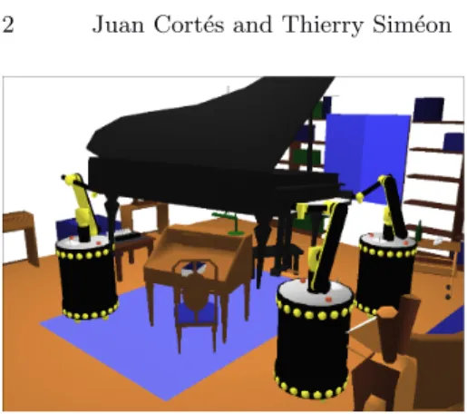
Complex articulated mechanisms with closed kinematic chains appear in all the domains where motion planning techniques can be applied. Figure 1 illustrates an example of coordinated manipulation of an object handled by several robots. The generality and the practical efficiency of the extended planners incorporating RLG allow to tackle such kind of problems as well as problems involving parallel robots, or problems arising in computational
Fig. 1. A “closed-chain” version of the piano mover’s problem. The pi-ano is moved by three cooperating mobile manipulators, creating multi-ple closed kinematic chains.
biology for the structural analysis of protein loops. All these applications are commented in Sect. 7. We conclude devising new directions for future research (Sect. 8).
2
Problem Formulation
The motion planning problem consists in finding a path between two given locations of a mobile system that satisfies intrinsic constraints as well as constraints that arise from the environment. Basically, motion constraints are due to the kinematic structure of the mechanism and to collision avoid-ance. Under these constraints, the problem can be posed and solved in the configuration-spaceC [19]. Then, it is reduced to explore the connectivity of the subsetCf ree of the collision-free configurations.
The problem has been clearly formulated for articulated mechanisms with-out kinematic loops (see [13] for a detailed formulation). In this case,C cor-responds to the space of the joint variables Q, called the joint-space. Topo-logically, Q is a smooth manifold, with a simple parameterization [2]. For an articulated mechanism with m independent joint variables defined in real intervals, Q can be seen as a m-dimensional hypercube. If the articulated mechanism contains closed kinematic chains, then some joint variables are related by loop-closure equations [20]. A general expression of loop-closure constraints is: f (Q) = I, where f(Q) is a system of non-linear equations and I is the identity displacement. The configuration-space C of a closed-chain mechanism is the subset of Q satisfying such equations. The stratification of C leads to several ρ-dimensional manifolds Mi which can be connected
through sets of lower dimension Sk [3,27]. Note that ρ corresponds to the
global mobility of the mechanism. TheMi are called self-motion manifolds
and the Sk are sets of singular configurations. The number of self-motion
manifolds is bounded, and it tends to decrease as ρ increases [3].
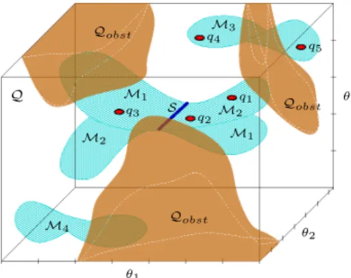
Figure 2 illustrates a fictive example with three joint variables{θ1, θ2, θ3}
and ρ = 2. Let us consider a function of the form f (θ1, θ2, θ3) = 0, representing
loop-closure constraints. This function maps to several surfaces embedded in the joint-spaceQ. Such surfaces are the different self-motion manifolds Mi. In
this example,M1andM2intersect at a singular setS. We have represented
the obstacle regionQobst in the joint-space.Qf ree is the complementary
Q q4 M1 M2 q5 q1 q2 Qobst Qobst Qobst θ1 θ3 θ2 M3 M4 S q3 M2 M1
Fig. 2. Illustration for the for-mulation of the motion planning problem under kinematic loop-closure constraints. Configurations are grouped into several subsets em-bedded in the joint-space.
Several situations can rise in motion planning queries within this example. The best case is a query for a path between q1 and q2. These configurations
lie on the same self-motion manifold and in the same connected component of Cf ree, thus there is a free path between them. A path is also feasible between
q1and q3, even if it contains singular configurations. However, for q4and q5,
the presence of obstacles makes these configurations cannot be connected by a free path. Finally, a case that does not appear for open kinematic chains can rise under closure constraints: q1and q4lie on the same connected component
ofQf ree but on different components of C !
3
Available Techniques
Only a few exact motion planning approaches have been proposed that treat kinematic loop-closure and collision avoidance simultaneously, including these two types of constraints within algebraic expressions (e.g. [4,1]). The compu-tational complexity of these approaches makes them unpractical. Normally, different techniques have to be combined for planning motions under kine-matic loop-closure constraints. First, loop-closure equations must be solved to obtain the configuration-space C. Then, motion planning algorithms can be applied to compute paths in the collision-free subsetCf ree.
Techniques that provide a complete solution of loop-closure equations are very limited in practice. Currently, they can be applied to non-redundant mechanisms, single loops with only a few (two or three) degrees of redun-dancy or particular classes of parallel mechanisms [22,21,23]. For more com-plex closed-chain mechanisms, only discrete points inC can be obtained. The use of a grid for globally representingC is not applicable to high-dimensional spaces. The remaining possibility is then to use sampling techniques com-bined with numerical or algebraic techniques to obtain single configurations satisfying loop-closure equations. This fact restrains the choice of motion planning algorithms to those based on sampling.
Sampling-based planners have demonstrated their efficacy for solving diffi-cult problems in high-dimensional spaces. The Probabilistic RoadMap (PRM) [12] and the Rapidly-exploring Random Trees (RRT) [16] are two approaches that have had a particular success. However, only two attempts had been made to extend such sampling-based planners to closed-chain mechanisms [15,11].
The first PRM-based approach able to handle mechanisms with closed chains was presented in [15]. The problem is formulated in the joint-spaceQ. Closure constraints are expressed by error functions involving distances in the Euclidean space. Numerical optimization techniques are used to sample and to connect configurations in the subset ofQ satisfying these constraints within a given tolerance. The approach is general but suffers the drawbacks of optimization-based methods to solve inverse kinematic problems: they are exposed to the local minima problem and the convergence can be very slow. A technique to randomly sample the tangent space of the constraints is pro-posed that increases the efficiency of the process to connect sampled config-urations. More details of the method and the extension of RRT-based algo-rithms were subsequently published in [29,30]. For the RRT approach, the random configurations used to bias the exploration are generated ignoring closure constraints. The argument is that computing closed configurations is too expensive and does not provide appreciable benefit. We will show in Sect. 6 that this last assertion is not totally right.
The approach described in [11] treats closed kinematic chains within a PRM-based planner. Each loop in the mechanism is broken into two sub-chains. For computing nodes, uniform random sampling is used to generate the configuration of one of the subchains (called active subchain) and then an inverse kinematics problem is solved to obtain the configuration of the remaining part of the loop (called passive subchain) in order to force closure. For computing edges, the local planner is limited to act on the active con-figuration parameters and the corresponding passive variables are computed for each intermediate configuration along the local path. For the efficiency of the roadmap computation, the passive subchain of each loop must be a non-redundant mechanism with closed-form inverse kinematics solution. As the authors admit, this means an important drawback when the approach is applied to a highly-redundant loop. The probability of randomly generating configurations of a long active subchain for which a configuration of the pas-sive chain satisfying closure constraints exists is very low. The performance of the algorithm drops off significantly due to this fact.
Our approach shares some ideas used for the extension of PRM-based planners in [11]. One of our contributions is to resolve the main drawback of the referred technique by the integration of the RLG sampling technique (explained in Sect. 5).
4
Sampling-Based Planning
and Closed-Chain Mechanisms
This section presents a general framework to extend sampling-based ap-proaches for planning the motions of general closed-chain mechanisms. The use of sampling-based planners is strongly justified since, for the kind of problems we address (see Sect. 7), there is no available technique providing a complete, exact representation of Cf ree. However, there are important
dif-ficulties for sampling and for checking the connectivity of configurations of closed-chain mechanisms. Next, we discuss how to deal with these difficulties.
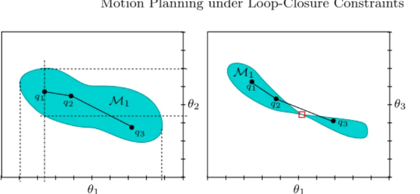
q1 q2 q3 q1 q3 q2 M1 θ2 θ3 M1 θ1 θ1
Fig. 3. Projection ofM1 on the planes θ1θ2 and θ1θ3.
On the Parameterization of C: Configurations of a closed-chain mech-anism are grouped into a finite number of lower-dimensional manifolds Mi
embedded in the joint-space Q (the search-space in our problem). These manifolds can be parameterized, at least locally, by a set of ρ independent parameters, selected from the joint variables. Points in the different man-ifolds can be generated by sweeping the ρ parameters through their range and evaluating the loop-closure equations that provide the value of the other (dependent) variables. An atlas of each one of these manifolds Mi can be
constituted by a finite number (in general not exceeding the dimension ofQ, m) of local charts considering different combinations of ρ parameters. With-out loss of generality, sets of ρ consecutive joint variables in a kinematic chain can be chosen as local coordinates [27].
Following a terminology also used in [11], we call active variables qa the
set of the ρ joint variables chosen as parameters of a local chart and passive variables qpthe remaining set of the m− ρ dependent joint variables, so that {qa, qp
} = q ∈ C ⊂ Q.
Main Principle: The core of our approach is to explore the connectivity of Cf reeby sampling configurations and by testing feasible connections through
local parameterizations ofC. Motion planning algorithms are applied on the local parameters qa. Using a roadmap method such as PRM, the nodes are
generated by sampling qa and local paths are obtained by applying a local planner (also called steering method) to these parameters. In a similar way, qa are the configuration parameters directly handled by incremental search
methods like RRT. Obviously, for each computed value of the parameters, loop-closure equations must be solved for obtaining the whole configuration of the mechanism q ∈ C. Therefore, the efficiency of the planner partially relies on the efficient solution of these equations.
Configuration Sampling: Given a set of active variables qa, loop-closure
equations have real solutions only for a range of values of each joint variable, that we call the closure range. Besides, the closure range of a parameter depends on the value of the other parameters. The last assertion is illustrated in Fig. 3, that shows the projection of the manifoldM1of Fig. 2 on the planes
θ1θ2 and θ1θ3. Let us consider qa={θ1, θ2} (the left image). If we sample
sampled in its whole closure range (i.e. the feasible range for any value of the other joint variables). However, θ2 is valid only in a subset of its whole
closure range, determined by the value of θ1.
There is no general and efficient method to define closure ranges of joint variables. Thus, in practice, the only possibility for sampling configurations is to use a trial method: sampling parameters qain the intervals defined for joint
variables and solving the loop-closure equations. Nevertheless, when a closure range is very restricted with respect to the interval of a joint variable, too many samples maybe tested before finding a feasible configuration. Hence, too much computing time is spent in solving closure equations leading to imaginary values. This is an important drawback for the efficiency of motion planners, and mainly for those using a roadmap approach, such as the planner in [11]. The RLG algorithm, further discussed in Sect. 5, resolves this problem using simple geometrical operations.
Computing Local Path: Sampling-based roadmap methods check the con-nectivity of nearby configurations by local paths. Incremental search methods try to expand a configuration toward a local goal, producing also a sort of local path. Such paths can be computed by explicitly variating the local pa-rameters qa and solving loop-closure equations with a given resolution for
obtaining qp.
Without a topological characterization ofC, the number of different sets of parameters qa required to determine if two configurations are connected
or not is a priori unknown. This fact can easily be understood on Fig. 3. Let us consider that a linear interpolation of the parameters qa produces a
kinematically feasible path (i.e. there are no differential constraints). Then, any two configurations lying onM1can be connected (directly or indirectly)
using qa=
{θ1, θ2} as local parameters. On the contrary, choosing qa={θ1, θ3}
leads to a non-complete solution of motion planning queries within M1. A
solution path between configurations q1and q2can be immediately obtained
since they are directly connected by a local path. However, a path between q1
and q3can not be found using sampling-based techniques. The point indicated
by the small square is a singularity of this parameterization. The probability of generating this point by sampling values of qa=
{θ1, θ3} is null, as well as
the probability of sampling two points on a line (local path) passing through this singularity. Thus, finding a feasible path between q1 and q3 requires
another set of local parameters than{θ1, θ3}.
Local paths have to satisfy other motion constraints besides loop-closure, such as collision avoidance. In this paper, we do not talk about these other constraints, that can be checked along local paths by techniques (e.g. [18]) similar to those used for open-chain mechanisms.
Dealing with Kinematic Singularities: Up to now we have limited our discussion to the case of a single manifold. However, C may be composed of several manifolds. These manifolds are either disjoint, or they intersect at lower-dimensional subsets corresponding to kinematically singular configu-rations. Therefore, exploring the connectivity of Cf ree requires to deal with
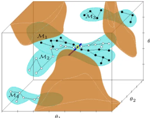
θ1 θ3 θ2 M2 M3 M4 M1
Fig. 4. Probabilistic roadmap cap-turing the connectivity ofCf ree for
the fictive motion planning problem involving kinematic closure con-straints of Sect. 2.
The roadmap represented in Fig. 4 has been built using qa={θ1, θ2} as
only set of parameters. Each point {θ1, θ2} maps to two configurations (i.e.
there are two solutions for qp= θ
3) on different manifolds for all the domain
underM1andM2except for the singular setS where they intersect, so that
configurations in these manifolds are connected by this singular set. This kinematic singularity corresponds to the singularity of the parameterization qa={θ1, θ3} commented above. It can be traversed by a local path on the
current parameterization. When a local path is computed between two con-figurations at different sides ofS, the bifurcation of the solution can be easily detected when checking the local path validity, and the singular configuration (marked by the small rectangle in Fig. 4) connecting M1 andM2 can then
be identified.
Let us consider now a more difficult case where M1 and M2 do not
intersect along a line but meet at a point. None of the three possible pa-rameterizations would allow to identify such a singular point exactly. The difference in this case is that the singular set has dimension ρ− 2 instead of ρ− 1. In theory, sets of kinematically singular configurations can have dimension from ρ− 1 to zero. Using sampling techniques for generating con-figurations onC and steering methods on subsets of configuration parameters qa, our approach has only the guarantee (if we do not admit a tolerance) to
find connections through singular sets of dimension ρ− 1. The other singular sets, from dimension ρ− 2 to isolated singularities, must be identified by other methods. The general treatment of such singularities goes beyond the scope of this paper. As far as we know, techniques able to globally charac-terize singular configurations have been proposed only for particular classes of mechanisms (e.g. [10,28]).
5
The RLG Algorithm
We have developed an algorithm, that we call Random Loop Generator (RLG), for sampling configurations of closed-chain mechanisms. The general approach was presented in [5]. Then, a variant that treats more efficiently parallel mechanisms was introduced in [6]. More details can be found in [7]. In this section, we present an overview containing main ideas.
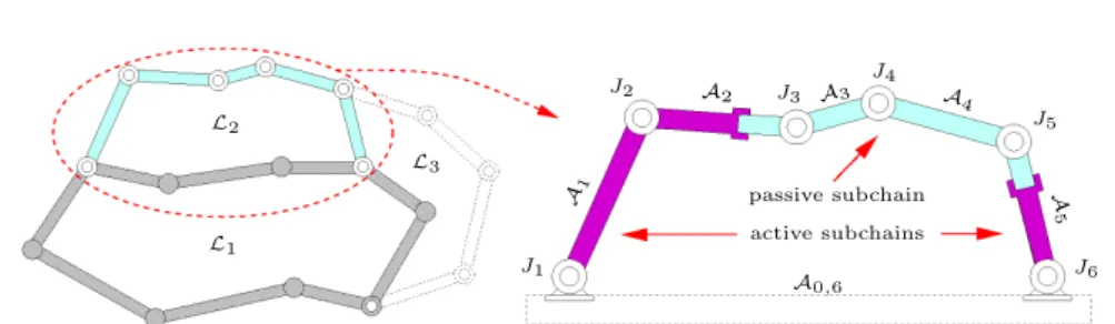
passive subchain active subchains L2 L1 L3 A 5 A4 A2 A0,6 A3 J6 A1 J3 J2 J1 J5 J4
Fig. 5. Decomposition of a multi-loop in single loops, and a possible choice of passive and active subchains in loopL2.
5.1 Mechanical System Decomposition
General Case: RLG is based on a decomposition of the mechanism into open kinematic chains. In the general case, single loops are handled sepa-rately, in a determined order. For each loop, sets of active and passive joint variables are defined consecutively such that they correspond to segments of the kinematic chain. We call passive subchain the segment involving the passive variables and active subchains to the other segments. There can be one or two active subchains depending on the placement of the passive sub-chain. The passive subchain is a non-redundant mechanism whose end-frame can span full-rank subsets of the workspace. In general, this requires three joint variables for a planar mechanism and six for a spatial mechanism. Effi-cient methods to solve inverse kinematics problems for such mechanisms are usually available [22].
In multi-loops, some joint variables are involved in the configuration of several individual loops. Their value is computed for the single loop treated first, and then, these common portions of the mechanism become rigid bodies when treating the other loops. Figure 5 shows an example of a planar multi-loop mechanism. The individual multi-loops are designated byLi, where the index
i indicates the order for the treatment. The figure also illustrates the decom-position of L2. This 6R planar linkage has mobility ρ = 3. Thus, qa and qp
contain three joint variables each. In this illustration we have chosen θ3, θ4
and θ5 (the variables associated with joints J3, J4 and J5) to be the passive
variables. Then, active variables can be seen as configuration parameters of two open chains rooted at a (fictive) link A0,6.
Parallel Mechanisms: A parallel mechanism is an articulated multi-loop structure in which a solid, the end-effector or platformP, is connected to the base A0 by at least two independent kinematic chains Ki. The pose of P is
defined by a vector qP ={xP, yP, zP, γP, βP, αP}. The three first elements
represent the position of FP relative to FA0, the frames associated with P and A0 respectively. The orientation is given by three consecutive rotations
around the coordinate axes of FP 1. We consider the configuration q of a parallel mechanism is defined by the platform pose and the configuration of the chainsKi: q ={qP, qK1, . . . , qKnk}. The parameters defining the platform
1
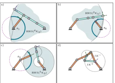
d) b) a) c) θ2 RWS(2K5) θ1 θ6 RWS(6K2) RWS(5K3) IK− IK+
Fig. 6. Steps of the RLG algorithm performing on a 6R planar linkage.
pose qP are selected as active variables. For a given platform pose, the base-frame and the end-base-frame of each chainsKi have fixed relative location. Thus,
they have to be treated as closed kinematic chains. If a chainKiis redundant,
it is decomposed in active and passive subchains as explained above for a single loop. Thus, we can separate joint variables as follows: qKi ={qa
Ki, q
p Ki}.
Hence, variables defining the configuration q of a parallel mechanism are divided into active and passive such that:
qa={qP, qKa1, . . . , q a Knk} , q p= {qpK1, . . . , qKp nk} 5.2 Sampling process
RLG performs a “guided”-random sampling for qathat notably increases the
probability of obtaining real solutions for qp when solving the loop-closure
equations. Figure 6 illustrates the process on a planar 6R linkage (the loop L2 in Fig. 5). The active joint variables are computed sequentially by the
function Sample qa detailed in Algorithm 1. The two active subchains are
treated alternately. The idea of the algorithm is to progressively decrease the complexity of the closed chain until only the configuration of the passive subchain, qp, remains to be solved (by inverse kinematics).
At each iteration, the function ComputeClosureRange returns a set of intervals Icwhich approximate the closure range of a joint variable, for a fixed
configuration of the portions of loop previously generated. The approximation must be conservative in the sense that no region of C is excluded for the sampling. This is required in order to guarantee any form of sampling-based completeness (e.g. probabilistic completeness) of motion planning algorithms. The value of the joint variable is randomly sampled inside the intervals Ic.
The problem of computing the closure range of a joint variable can be for-mulated as follows. Given a closed kinematic chainbK
einvolving joints from
Algorithm 1: Sample qa
input : the loopL output : the parameters qa begin
1 (Jb, Je)← InitSampler(L);
while not EndActiveChain(L, Jb)do
Ic← ComputeClosureRange(L, Jb, Je);
if Ic=∅ then goto line 1;
SetJointValue(Jb, Random(Ic));
Jb← NextJoint(L, Jb);
if not EndActiveChain(L, Je)then Switch(Jb, Je);
end
are obtained by breaking the linkAbbetween Jb and Jb+1. A suitable
break-point is the physical placement of Jb+1, but any other point can be chosen.
A frame Fcassociated with this break-point can be seen as the end-frame of
both open chains. The closure range of the joint variable corresponding to Jb is the subset of values making Fc reachable by the chain eKb+1. Solving
such a problem requires to represent the workspace of this chain, which is in general very complicated. For our purpose, a simple and fast method is pre-ferred versus a more accurate but slower one. RLG handles simple volumes that bound the reachable workspace (i.e. only considering positional reacha-bility). They are denoted by RWS in Fig. 6. In general, a reasonable choice for the RWS is a spherical shell with external and internal radii correspond-ing respectively to an upper bound of the maximum extension and a lower bound of the minimum extensions of the chain. Once defined RWS(eK
b+1),
computing the approximation of the closure intervals for Jbis very simple. If
Jb is a revolute joint, then the origin of Fc describes a circle around its axis.
If Jb is a prismatic joint, the origin of Fc moves on a straight-line segment.
Then, Ic is obtained from the intersection of a circle or a line with a simple
volume RWS.
The function to sample qP for a parallel mechanism is based on the same principle that Sample qa. The parameters are sampled progressively from
the computed closure range approximations. The main difference is that the closure range depends now on the satisfaction of closure constraints that simultaneously involve several individual loops.
6
Performance of RLG
RLG is a general technique, applicable to any sampling-based planner. In this section, we show examples of motion planning problems solved by PRM and RRT planners extended to handle loop-closure constraints. The goal of the experiments is to compare the performance of the planners with and without incorporating RLG. The tests have been made with the software Move3D [25], in which our algorithms have been implemented.
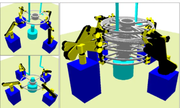
Fig. 7. Motion planning problem for four robotic arms manipulating an object. Start and goal configurations (left) and trace of the solution path (right).
6.1 Results with a PRM-based Planner
PRM-based algorithms build a graph (the roadmap) whose nodes are ran-domly sampled configurations that satisfy motion constraints. For a closed-chain mechanism, only the parameters qaare sampled, and loop-closure
equa-tions have to be solved to determine if the sample yields a valid configuration or not. We have compared the performance of the planner using an uniform random sampling2 or RLG for sampling qa.
Figure 7 shows four manipulators handling an object. The whole system can be seen as an articulated parallel structure. If the grasps are modeled as fixed attachments, the composed mechanism involves m = 30 joint variables (6 for each manipulator and 6 for the movable object), and the mobility is ρ = 6. Since the manipulators are non-redundant, qa = q
P: the parameters
defining the location of the object. Almost all (more than 90%) the con-figurations qP generated by RLG make the object simultaneously reachable by the four manipulators. Using a uniform random sampling, the bounds of the parameters qP have first to be adjusted “by hand” with relation to the workspace of the manipulators (this is not necessary for RLG). Even with a good setting of the bounds, less than 0.05% of the samples yield valid (closed) configurations. Let us see now the repercussion when solving motion plan-ning problems using the PRM approach. In the problem illustrated in the figure, the manipulators have to unhook an object and to insert it into the cylindrical axis. For computing a roadmap containing the solution path to this problem, millions of poses generated by uniform random sampling were necessary and the process took more than 20 minutes3. Using RLG for
sam-pling configurations, less than 500 random platform poses were generated and the roadmap was built in less than 20 seconds. This result show that RLG avoids an enormous number of futile operations (i.e. calls to inverse kinematics functions) which drop off the performance of the planner.
2
Implemented using the rand() function of the GNU C Library.
3
Tests were performed using a Sun Blade 100 Workstation with a 500-MHz UltraSPARC-IIe processor.
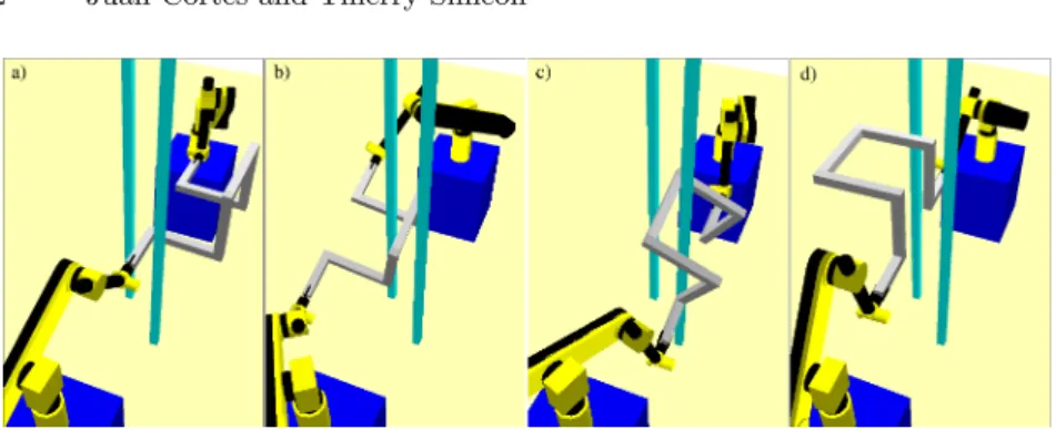
Fig. 8. Sequence of the solution to a difficult motion planning problem for two robotic arms manipulating an object among obstacles. 6.2 Results with an RRT-based Planner
The principle of RRT is to use uniformly distributed configurations qrand,
sampled at random inC, to bias the expansion of search trees in Cf ree. Under
loop-closure constraints, the use of samples in Q was proposed in [29] in order to evade the cost of sampling C. We have compared the performance of a uniform random sampling inQ versus RLG for generating qa
rand.
In the example illustrated in Fig. 8, two robotic arms coordinate for ma-nipulating a twisted bar among two vertical bars that restrict its motion. The goal is to solve a motion planning query between configurations in Fig. 8.a and Fig. 8.d. The figure shows a sequence of intermediate configurations of the solution of this puzzle-like problem. The difficulty of this problem de-pends on the distance between the vertical bars dbars. We have made tests
with three settings: dbars={150, 175, 200}. In this example, qacorresponds to
the configuration of one of the arms grasping the bar. The next table shows averaged results of tests. N is the number of iterations for expanding the search trees. T is the computing time. These results show the importance of an appropriate sampling considering the presence of kinematic loops. The gain obtained using the RLG sampling technique increases with the difficulty of the motion planning problem.
dbars Uniform With RLG N T N T gain T 200 2719 42.26 118 3.23 × 13 175 4995 102.92 424 6.30 × 16 150 9761 312.76 615 9.14 × 34
7
Applications of Closed-Chain Motion Planning
We have studied some of the possible applications of algorithms for motion planning under loop-closure constraints. One of them, coordinated manipu-lation planning, has been illustrated with the two examples in Sec. 6 and the problem shown in Fig. 1. This last problem combines several types of diffi-culty. First, the virtual structure composed by the three mobile manipulators grasping the piano can be seen as a parallel mechanism with redundant legs
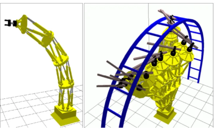
Fig. 9. Model of the robot Logabex-LX4, composed of four Gough-Stewart platforms connected in series, and trace of a collision-free path.
(the chainsKi correspond to the mobile manipulators). And second, the
ge-ometric complexity of the scene makes collision checking very hard. Besides, obstacles are strategically placed in order to hinder the motion of robots for changing the orientation of the piano. A roadmap that permits to solve most possible queries in this scene was computed using the an extended version of the Visibility-PRM algorithm [24] in 5 minutes.
Applied to parallel robots, motion planning algorithms can help designers of these mechanisms, or can provide useful data for real-time trajectory plan-ning. Our work on parallel mechanisms [6] represents the first effective appli-cation of sampling-based planners to this kind of articulated structures. The generality of our approach is demonstrated by the complexity of the systems that it is able to treat, such as the model of the Logabex-LX4 (Fig. 9), whose configuration-space is a 25-dimensional variety embedded in a 97-dimensional joint-space. Planning queries for moving the manipulator with the grasped bar from one to another opening of the bridge were solved by the extended RRT-based algorithm in less than one minute.
The above expounded closed-chain planners can also be used as a key component of a novel manipulation planning approach described in [26]. The clever idea is to explore the connectivity of the subset where the manipula-tion sub-paths (i.e. transit and transfer paths) meet via a virtual closed-chain mechanism consisting of the robot grasping the movable object placed at a stable position. Our manipulation planner automatically generates, among continuous sets, the grasps and the intermediate placements of the movable object required to solve complicated problems. It is the first general manip-ulation planner with this capability.
We also began to investigate applications out of the field of robotics. Mo-tion planning techniques can be used as new tools to help the resoluMo-tion of important open problems in computational biology [9]. We discuss in [8] the application of closed-chain planning techniques to the structural analysis of protein loops. The algorithms that we have presented can act as efficient fil-ters for conformational search methods by making a geometric treatment of strong energetic constraints: maintaining the backbone integrity (i.e.
loop-Fig. 10. Simulated conformational gating of loop 7 in amylosucrase. Crys-tallographic conformation (left) and geometrically feasible change (right). closure) and avoiding steric classes. We have developed a conformational sampling algorithm that provides random conformations achieving such ge-ometric constraints. The algorithm combines RLG for generating the back-bone conformation with other sampling and collision detection techniques to obtain feasible conformations of the side-chains. We also propose a new con-formational search technique, inspired by the RRT approach, for studying geometrically feasible loop motions. Preliminary results are promising. They demonstrate the capacity of the techniques to handle protein models with long loops that involve several dozens of degrees of freedom in the backbone and in the side-chains. Figure 10 illustrates an example of such a long loop in the model of amylosucrase from Neisseria polysaccharea.
8
Conclusions and Future Work
We have introduced sampling-based motion planning algorithms into an ex-tended formulation of the motion planning problem under kinematic loop-closure constraints. We have tried to give general directives without focusing on a particular implementation. The RLG algorithm allows to overcome the challenge of sampling random configurations for general closed-chain mecha-nisms. The results obtained, in different domains of application, when solv-ing difficult problems with PRM-based and RRT-based extended planners, demonstrate the efficacy and the generality of the approach.
Several points remain for future research. Some of them concern the RLG sampling algorithm. RLG provided good results in all our experiments. Nev-ertheless, a deeper analytical work is necessary in order to characterize its performance. Also, studying new forms of sampling, using quasi-random se-quences or multi-resolution grids recently proposed [17], seems to be an in-teresting way to follow. Another improvement involves the selection of active and passive subchains. A general automatic method, based on an analysis of kinematic diagrams of mechanisms, remains to be devised.
A general methodology for the treatment of singularities within sampling-based motion planning algorithms remains an open topic to be further in-vestigated. Recent interval methods [21,23] appear to be another matter to
study for the improvement of closed-chain motion planning techniques. In-terval methods can provide a complete approximated representation of the whole set of configurations satisfying loop closure equations. They compute a set of boxes that contain the continuum of solutions. Such a representa-tion is very suitable for the applicarepresenta-tion of sampling-based morepresenta-tion planning algorithms.
Another direction for future research concerns the application of closed-chain motion planning to computational biology. We intend to further study problems in structural biology that require the development of new tech-niques for the conformational analysis of protein loops. A first goal is to get efficient algorithms to capture the whole subset of the geometrically feasible conformations of one or several loops in the same protein. The next goal is to handle several proteins that interact while changing the conformation of loops on their surfaces. Applications to structural biology are attractive for the algorithmic development because of the kinematic complexity of molecular models. Obviously, robotic applications could also benefit from improvements achieved in this field.
Acknowledgments.
This work has been supported by the European project IST-37185 MOVIE and the project BioMove3D of the CNRS Bioinformatics Research Program.
References
1. Basu S., Pollack R., Roy M.-F. (2000). Computing Roadmaps of Semi-algebraic Sets on a Variety. J. Am. Math. Soc. 13(1), 55–82
2. Burdick J.W. (1988). Kinematic Analysis and Design of Redundant Robot Ma-nipulators. PhD Thesis, Stanford University.
3. Burdick J.W. (1989). On the Inverse Kinematics of Redundant Manipulators: Characterization of the Self-Motion Manifold. Proc. IEEE Int. Conf. Rob. & Autom., 264–270
4. Canny J.F. (1988). The Complexity of Robot Motion Planning. MIT Press, Cambridge
5. Cort´es J., Sim´eon T., Laumond J.-P. (2002). A Random Loop Generator for Planning the Motions of Closed Kinematic Chains using PRM Methods. Proc. IEEE Int. Conf. Rob. & Autom., 2141–2146
6. Cort´es J., Sim´eon T. (2003). Probabilistic Motion Planning for Parallel Mech-anisms. Proc. IEEE Int. Conf. Rob. & Autom., 4354–4359
7. Cort´es J. (2003). Motion Planning Algorithms for General Closed-Chain Mech-anisms. PhD Thesis, Institut National Polytechnique de Toulouse
8. Cort´es J., Sim´eon T., Remaud-Sim´eon M., Tran V. (2004). Geometric Algo-rithms for the Conformational Analysis of Long Protein Loops. J. Comp. Chem. 25(7), 956–967
9. Finn P.W., Kavraki L.E., Latombe J.-C. et al. (1998). RAPID: Randomized Pharmacophore Identification. Comp. Geom.: Theory & Appl. 10(4), 263–272 10. Gosselin C. (1988). Kinematic Analysis, Optimization and Programming of
11. Han L., Amato N.M. (2001). A Kinematics-Based Probabilistic Roadmap Method for Closed Kinematic Chains. In: Donald B.R., Lynch K.M., Rus D. (Eds.) Algorithmic and Computational Robotics: New Directions (WAFR2000). A.K. Peters, Boston, 233–245
12. Kavraki L.E., Svestka P., Latombe J.-C., Overmars M.H. (1996). Probabilistic Roadmaps for Path Planning in High-Dimensional Configuration Spaces. IEEE Trans. Rob. & Autom. 12(4), 566–580
13. Latombe J.-C. (1991). Robot Motion Planning. Kluwer Academic Publishers 14. Latombe J.-C. (1999). Motion Planning: A Journey of Robots, Molecules,
Dig-ital Actors, and Other Artifacts. Int. J. Rob. Res. 18(11), 1119–1128
15. LaValle S.M., Yakey J.H., Kavraki L.E. (1999). A Probabilistic Roadmap Ap-proach for Systems with Closed Kinematic Chains. Proc. IEEE Int. Conf. Rob. & Autom., 473–479
16. LaValle S.M., Kuffner, J.J. (2001). Rapidly-Exploring Random Trees: Progress and Prospects. In: Donald B.R., Lynch K.M., Rus D. (Eds.) Algorithmic and Computational Robotics: New Directions (WAFR2000). A.K. Peters, Boston, 293–308
17. LaValle S.M., Branicky M.S. (2004). On the Relationship Between Classical Grid Search and Probabilistic Roadmaps. In: Boissonnat J.-D., Burdick J., Goldberg K., Hutchinson S. (Eds.). Algorithmic Foundations of Roadmaps V (WAFR2002). Springer-Verlag, Berlin, 59–75
18. Lin M.C., Manocha D. (2004). Collision and Proximity Queries. In: Hand-book of Discrete and Computational Geometry: Collision Detection. To appear. Available at http://www.cs.unc.edu/∼dm/
19. Lozano-P´erez, T. (1983). Spatial Planning: A Configuration Space Approach. IEEE Trans. Computers 32(2), 108–120
20. McCarthy J.M. (2000). Geometric Design of Linkages. Springer-Verlag, New York
21. Merlet J.-P. (2001). A Parser for the Interval Evaluation of Analytical Functions and its Applications to Engineering Problems. J. Symb. Comp. 31, 475–486 22. Nielsen J., Roth B. (1997). Formulation and Solution for the Direct and Inverse
Kinematics Problem for Mechanisms and Mechatronic Systems. Proc. NATO Adv. Study Inst. on Comp. Meth. in Mech. 1, 233–252
23. Porta J.M., Ros L., Thomas F., Torras C. (2003). A Branch-and-Prune Algo-rithm for Solving Systems of Distance Constraint. Proc. IEEE Int. Conf. Rob. & Autom., 342–348
24. Sim´eon T., Laumond J.-P., Nissoux C. (2000). Visibility-Based Probabilistic Roadmaps for Motion Planning. Adv. Rob. J. 14(6), 477–494
25. Sim´eon T., Laumond J.-P., Lamiraux F. (2001). Move3D: a Generic Platform for Path Planning. Proc. IEEE Int. Symp. Assembly & Task Planning, 25–30 26. Sim´eon T., Laumond J.-P., Cort´es J., Sahbani A. (2004). Manipulation
Plan-ning with Probabilistic Roadmaps. Int. J. Rob. Res., in press
27. Thomas F. (1993). The Self-Motion Manifold of the N-bar Mechanism. In: Angeles J., Hommel G., Kov´acs P. (Eds.) Computational Kinematics. Kluwer Academic Publishers, Dordrecht, 95–107
28. Trinkle J.C., Milgram R.J. (2002). Complete Path Planning for Closed Kine-matic Chains with Spherical Joints. Int. J. Rob. Res. 21(9), 773–789
29. Yakey J.H. (2000). Randomized Path Planning for Linkages with Closed Kine-matic Chains. MA Thesis, Iowa State University
30. Yakey J.H., LaValle S.M., Kavraki L.E. (2001). Randomized Path Planning for Linkages with Closed Kinematic Chains. IEEE Trans. Rob. & Autom. 17(6), 951–958