Tropopause referenced ozone climatology and inter-annual variability (1994–2003) from the MOZAIC programme
49
0
0
Texte intégral
Figure


+7


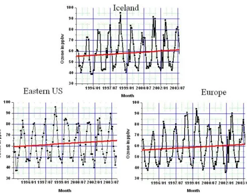
![Fig. 6 : Comparison over the three selected regions of the ozone seasonal cycles recorded at the tropopause and a theoretical sine variation defined for every month as O3(month) = 91 + 28*sin[Pi*(month-2)/6]](https://thumb-eu.123doks.com/thumbv2/123doknet/2338833.33450/37.918.709.897.76.632/comparison-selected-regions-seasonal-recorded-tropopause-theoretical-variation.webp)
Documents relatifs
