An Approach for Aerodynamic Optimizaton of Transonic Fan Blades

(1)

AN APPROACH FOR AERODYNAMIC OPTIMIZATION OF TRANSONIC

FAN BLADES

MARYAM KHELGHATIBANA DÉPARTEMENT DE GÉNIE MÉCANIQUE ÉCOLE POLYTECHNIQUE DE MONTRÉAL

MÉMOIRE PRESENTÉE EN VUE DE L’OBTENTION DU DIPLÔME DE MAÎTRISE ÈS SCIENCES APPLIQUÉES

(GÉNIE MÉCANIQUE) JUIN 2014

(2)

UNIVERSITÉ DE MONTRÉAL

ÉCOLE POLYTECHNIQUE DE MONTRÉAL

Ce mémoire intitulé:

AN APPROACH FOR AERODYNAMIC OPTIMIZATION OF TRANSONIC FAN BLADES

presentée par : KHELGHATIBANA Maryam

en vue de l’obtention du diplôme de : Maîtrise ès sciences appliquées a été dûment accepté par le jury d’examen constitué de :

M. VO, Huu Duc, Ph.D., président.

M. TRÉPANIER, Jean-Yves, Ph.D., membre et directeur de recherche. M. REGGIO, Marcelo, Ph.D., membre.

(3)

DEDICATION

(4)

ACKNOWLEDGEMENTS

First and foremost, I would like to express my sincere gratitude to my supervisor, Prof. Jean-Yves Trépanier, for accepting me in IDEA chair and also for his continuous support and encouragement during my Masters study.

My sincere thank also goes to my co-supervisor, Dr. Christophe Tribe, for his invaluable advices which guided me through this research work.

I wish to express my gratefulness to Eddy Petro, research assistant at École Polytechnique de Montréal, who has indeed generously provided me with his experience and vast knowledge in computational fluid dynamics.

Moreover, I would like to acknowledge the support of the industrial partner of this project, Pratt & Whitney Canada. I sincerely thank Jason Nichols for his support and advice during this research work.

I would like to thank my colleague Saima Naz, Ph.D student in MDO project, for the useful discussion and collaboration that we had. I also would like to thank Radouan Boukharfane, Martin Gariepy, Benoit Malouin and Sami Ammar for helping me in learning French and integrating with my new hometown, Montréal.

Last but not the least; I would like to thank my family for all their love and support, specially my sister Leila who has been my greatest supporter during my stay in Montréal.

(5)

RÉSUMÉ

L'optimisation de la soufflante du moteur est une procédure longue et complexe à cause de la complexité du champ d'écoulement à l'intérieur du soufflante, les exigences contradictoires de conception et l'espace de conception de grande dimension. Afin de répondre à tous ces défis, une méthode d'optimisation aérodynamique des pales des soufflantes des moteurs transsoniques a été développée dans ce projet. Cette méthode automatise le processus de conception en intégrant une méthode de paramétrage géométrique, un solveur CFD et des méthodes d'optimisation numérique. Cette méthode peut être appliquée à la fois à des problèmes de conception à un ou plusieurs points de design. Une paramétrisation multi-niveau pour les pales de soufflantes transsoniques a été utilisée pour modifier la géométrie des pales. Des analyses numériques sont effectuées par la résolution des équations 3D Reynolds-Averaged Navier-Stokes combiné avec un modèle turbulence SST. Les algorithmes génétiques et les méthodes d'optimisation hybrides sont appliquées pour résoudre le problème d'optimisation. Afin de vérifier l'efficacité et la faisabilité de la méthode d'optimisation, un problème d'optimisation visant à maximiser l'efficacité du point de design a été formulé et appliqué dans le but de redesigner un cas de test. Cependant, la conception des pales de soufflantes transsoniques est en soi un problème à multiples facettes qui traite de plusieurs objectifs tels que l'efficacité, la marge de pompage, et la marge d’étranglement. La méthode d'optimisation multi-point proposée dans l'étude actuelle est formulée comme un problème bi-objectif dans le but de maximiser les efficacités du point de design et au point près du décrochage tout en maintenant le rapport de pression au point de design. L'amélioration de ces objectifs se détériore de manière significative au niveau de la marge d’étranglement, en particulier à des vitesses de rotation élevées. Par conséquent, une autre contrainte est intégrée dans le problème d'optimisation en vue de prévenir la réduction de la marge d’étranglement à des vitesses élevées. Étant donné que la localisation du début du décrochage est numériquement très coûteuse, la marge de pompage n'a pas été considérée comme un objectif dans l'énoncé du problème. Cependant, l'amélioration de l'efficacité à la condition d’opération proche du décrochage entraîne une meilleure performance à la condition de décrochage qui pourrait améliorer la marge de pompage. Une enquête est donc effectuée sur les solutions Pareto-optimales pour démontrer la relation entre l'efficacité aux conditions près du décrochage et de la marge de pompage.

(6)

La méthode proposée est appliquée pour redesigner le rotor NASA 67 pour les conditions de fonctionnement à un et plusieurs points. L'optimisation de la conception à un seul point a montré une amélioration de +0,28 points de l'efficacité isentropique au point de design tandis que le rapport de pression de design et le débit de masse présentent respectivement des écarts relatifs de moins de 0,12% et 0,11% par rapport aux valeurs pour la pale de référence. Deux cas d’optimisation point sont effectués: d'abord, le problème proposé d'optimisation multi-point est détendu en supprimant la contrainte de marge de d’étranglement afin de démontrer la relation entre l'efficacité au point près du décrochage et la marge de pompage. Une enquête sur les solutions Pareto-optimale de cette optimisation montre que la marge de décrochage a été augmentée avec l'amélioration de l'efficacité près du décrochage. Le second cas d'optimisation multi-point est effectué en tenant compte de tous les objectifs et contraintes. Un design optimisé sélectionné sur le front de Pareto présente une amélioration respectivement de +0.41, +0.56 et +0.9 points de l’efficacité à condition de design, de l’efficacité près du décrochage et de la marge de décrochage. Le rapport de pression et le débit massique à la condition de design présentent respectivement des écarts relatifs de moins de 0,3% et 0,26% par rapport aux valeurs pour la pale de référence. En outre, la pale optimisée maintient la marge d’étranglement nécessaire. Les analyses aérodynamiques détaillées sont effectuées pour étudier l'effet de l'optimisation de la géométrie de la pale sur la présence du choc, les écoulements secondaires, l’écoulement de jeu et l`interactions entre les chocs et l’écoulement de jeu pour les optimisations à un ou plusieurs points.

(7)

ABSTRACT

Aerodynamic design optimization of transonic fan blades is a highly challenging problem due to the complexity of flow field inside the fan, the conflicting design requirements and the high-dimensional design space. In order to address all these challenges, an aerodynamic design optimization method is developed in this study. This method automates the design process by integrating a geometrical parameterization method, a CFD solver and numerical optimization methods that can be applied to both single and multi-point optimization design problems. A multi-level blade parameterization is employed to modify the blade geometry. Numerical analyses are performed by solving 3D RANS equations combined with SST turbulence model. Genetic algorithms and hybrid optimization methods are applied to solve the optimization problem. In order to verify the effectiveness and feasibility of the optimization method, a single-point optimization problem aiming to maximize design efficiency is formulated and applied to redesign a test case. However, transonic fan blade design is inherently a multi-faceted problem that deals with several objectives such as efficiency, stall margin, and choke margin. The proposed multi-point optimization method in the current study is formulated as a bi-objective problem to maximize design and near-stall efficiencies while maintaining the required design pressure ratio. Enhancing these objectives significantly deteriorate the choke margin, specifically at high rotational speeds. Therefore, another constraint is embedded in the optimization problem in order to prevent the reduction of choke margin at high speeds. Since capturing stall inception is numerically very expensive, stall margin has not been considered as an objective in the problem statement. However, improving near-stall efficiency results in a better performance at stall condition, which could enhance the stall margin. An investigation is therefore performed on the Pareto-optimal solutions to demonstrate the relation between near-stall efficiency and stall margin.

The proposed method is applied to redesign NASA rotor 67 for single and multiple operating conditions. The single-point design optimization showed +0.28 points improvement of isentropic efficiency at design point, while the design pressure ratio and mass flow are, respectively, within 0.12% and 0.11% of the reference blade. Two cases of multi-point optimization are performed: First, the proposed multi-point optimization problem is relaxed by removing the choke margin constraint in order to demonstrate the relation between near-stall efficiency and stall margin. An investigation on the Pareto-optimal solutions of this optimization

(8)

shows that the stall margin has been increased with improving near-stall efficiency. The second multi-point optimization case is performed with considering all the objectives and constraints. One selected optimized design on the Pareto front presents +0.41, +0.56 and +0.9 points improvement in near-peak efficiency, near-stall efficiency and stall margin, respectively. The design pressure ratio and mass flow are, respectively, within 0.3% and 0.26% of the reference blade. Moreover the optimized design maintains the required choking margin. Detailed aerodynamic analyses are performed to investigate the effect of shape optimization on shock occurrence, secondary flows, tip leakage and shock/tip-leakage interactions in both single and multi-point optimizations.

(9)

LIST OF TABLES

Table 3.1 Design specifications of NASA rotor 67 [42] ... 20

Table 3.2 Design variables and their bounds ... 24

Table 4.1 Performance comparison between the reference blade and optimized blade ... 43

Table 4.2 Performance comparison between the reference blade and optimized blade ... 50

Table 4.3 Performance comparison between the reference and optimized blades ... 53

(12)

LIST OF FIGURES

Figure 1.1 Schematic of a fan map ... 2

Figure 2.1 Pareto front and principle of dominance ... 9

Figure 3.1 Flowchart of automatic design optimization ... 19

Figure 3.2 NASA rotor 67 [42] ... 20

Figure 3.3 Distribution of β-angle (Left) and Thickness (Right) in axial and spanwise directions [3] ... 23

Figure 3.4 Application of multi-level module ... 23

Figure 3.5 Computational domain and boundary conditions ... 25

Figure 3.6 Mesh independency study ... 26

Figure 3.7 Computational grid ... 27

Figure 3.8 Trend for streamwise y+ at (a) 10% (b) 50% (c) 90% of span ... 28

Figure 3.9 Comparison of performance curve of the coarse mesh and the fine mesh ... 30

Figure 3.10 Comparison of Mach contours of the coarse mesh and the fine mesh at 90% span at near peak efficiency and near stall conditions... 30

Figure 3.11 Aerodynamic survey locations ... 33

Figure 3.12 Fan map comparison of NASA rotor67 generated by Ansys CFX simulation with experimental data (1.2 million mesh) ... 33

Figure 3.13 Comparison of near peak efficiency Mach contours of NASA rotor 67 between experimental data and Ansys CFX simulation (1.2 million mesh)... 34

Figure 3.14 Comparison of near stall Mach contours of NASA rotor 67 between experimental data and Ansys CFX simulation (1.2 million mesh)... 35

Figure 3.15 Operating Points ... 37

Figure 4.1 Single-point optimization convergence plot ... 42 Figure 4.2 Comparison of blade geometry between the reference blade and the optimized blade 42

(13)

Figure 4.3 Operating characteristics of the reference and the optimized blades (a) total pressure

ratio and (b) isentropic efficiency ... 43

Figure 4.4 Isentropic Mach number distribution at (a) 10%, (b) 50% and (c) 90% of span ... 45

Figure 4.5 Wall shear stress streamlines on the blade suction side... 46

Figure 4.6 Optimization convergence analysis (obtained from the optimization on the coarse mesh) ... 48

Figure 4.7 Optimization objective design space (results obtained from the optimization on the coarse mesh) ... 48

Figure 4.8 Investigation of the relation between near stall point efficiency and stall margin (results obtained from the coarse mesh) ... 49

Figure 4.9 Comparison of blade geometry between the reference blade and optimized blade ... 50

Figure 4.10 Optimization convergence analysis ... 52

Figure 4.11 Optimization objective design space ... 52

Figure 4.12 Comparison of blade geometry between the reference blade and optimized blade ... 53

Figure 4.13 Operating characteristics of the reference and the optimized blades (a) total pressure ratio and (b) isentropic efficiency ... 55

Figure 4.14 Isentropic Mach number distribution at (a) 10%, (b) 50% and (c) 90% of span at OP1 ... 56

Figure 4.15 spanwise distributions of (a) temperature ratio (b) pressure ratio, and (c) flow angle at the rotor blade outlet at OP1 ... 57

Figure 4.16 Wall shear stress streamlines on the blade suction side ... 59

Figure 4.17 Pressure contours on the blade pressure surface ... 59

Figure 4.18 Relative Mach number contour at a) 40%, b) 60% and c) 80% of chord at OP1 ... 60

Figure 4.19 Relative Mach number contour at a) 40%, b) 60% and c) 80% of chord at OP2 ... 61

Figure 4.20 Contours of relative Mach number on a blade-to-blade stream surface at 90% span at OP1 ... 63

(14)

Figure 4.21 Contours of relative Mach number on a blade-to-blade stream surface at the blade tip

at OP1 ... 64

Figure 4.22 trade-off analyses for single-point optimization... 66

Figure 4.23 Trade-off study between efficiency at OP1 and mass flow at OP3 ... 67

(15)

NOMENCLATURE

CFD Computational Fluid Dynamics

Eff Efficiency

Total enthalpy

LE Leading Edge

Mass flow rate

Exit corrected mass flow

M Mach number

NSGA-II Non-dominated Sorting Genetic Algorithm Total pressure

Standard pressure at sea level

PR Pressure Ratio

pcm Position of the control points for the β-angle distribution pcl Position of the control points for the thickness distribution PSO Particle Swarm Optimization

RANS Reynolds-Averaged Navier-Stokes

Ref Reference

s length of the arc of the suction side

SA Simulated Annealing

SM Stall Margin

SST Shear Stress Transport Total temperature

TE Trailing Edge

(16)

rpm Round per minute

R67 NASA rotor67

β-angle Angle between the tangent of the curve and the meridional direction Modification on β-angle

Derivative of β-angle with respect to s Modification on Isentropic efficiency @ At 1D One-dimensional 2D Two-dimensional 3D Three-dimensional

(17)

LIST OF APPENDICES

APPENDIX A………76 APPENDIX B………78

(18)

CHAPTER 1 INTRODUCTION

1.1 Background

A fan is a low pressure compressor in the compressor set of a turbofan engine and is responsible to generate the major part of the engine’s thrust. The aerodynamic performance of a fan can be presented in a fan map which is composed of a set of characteristic curves called speedlines as shown in Figure 1.1. Each of the speedlines is the plot of the variation of pressure rise (pressure ratio or pressure rise coefficient) with the flow rate across the fan for a constant rotational speed. For each speedline, the variation of efficiency can also be plotted as shown in Figure 1.1. The line along which the fan operates as the engine is slowly accelerated or decelerated is called the working line. The intersection of the working line with the speedline at design rotational speed is the design point of the fan which should be at or close to the peak efficiency point. The left- and right-hand extremities of the speedlines are limited by the occurrence of stall and choke conditions, respectively. As the flow rate through the fan is reduced to small values, the incidence angle increases on the rotor blade and results in boundary layer separation and aerodynamic instabilities in the form of rotating stall. Rotating stall is the formation of a cell of velocity deficiency that rotates at 15-50% of the compressor rotor speed [1] and results in drops in pressure rise and efficiency of the fans. The leftmost point on a speedline is called stall point. The stall points of the speedlines may be joined up to form the stall line. The margin between the stall line and working line is known as stall margin. At high mass flow rates the occurrence of sonic conditions in the throat of the rotor results in choked flow. At choke limit, any further increase in the mass flow results in a rapid drop in efficiency and pressure ratio. The difference in flow value between choke condition and design point is called choke margin.

(19)

Figure 1.1 Schematic of a fan map

1.2 Problem definition

The aerospace industry has faced a continuous growth in the past few decades. This has led aircraft engine manufacturers to continuously seek for more competitive products in terms of efficiency, weight, durability, and cost. Transonic fans are widely used nowadays since they reduce the weight and size of the engine by elevating the pressure ratio per stage. The high speed flow in these types of fans, however, usually leads to strong shock waves at the blade tip, which results in losses and thus reduced efficiency. Limited stability margin is another characteristic of transonic fans, such that the range of stable operation at the design point is often as little as 10 percent of the design flow [2]. Today, the performance of these machines has reached a high level and the potential gains are relatively small. However, even a very small improvement of performance can result in a large economic savings over the lifetime of an engine.

Designing transonic fan blades is a highly complex and iterative task which involves several disciplines such as aerodynamics, structure and dynamics. Aerodynamics is usually considered as the initial phase of the design and thereby, it has a key role in achieving a good final design. The aerodynamic design problem starts with considering design requirements at design point. However, since aircraft engines will be operated over a wide range of conditions, it is essential to consider off-design analysis in designing fan blades. The performance of the fans at

(20)

stall condition and also the operating flow range at high speeds are particularly important when improving off-design performance. The objectives involved in turbomachinery blade design are contradicting. For example, improving the performance of the blade at design point results in a deterioration of near-stall performance, or improving stall margin may lead engine to choke at a lower mass flow rate. The aerodynamic design of fan blades has been traditionally performed by knowledgeable and skillful engineers who used know-how and cut-and-try approaches. However, these approaches are very time-consuming. Moreover, even for a skillful designer it is very difficult (and maybe impossible) to find a wide range of trade-offs between the different design requirements. Nowadays, the presence of high-speed computers allows the engineers to benefit from design optimization process where a set of selected design variables are varied automatically by an optimization algorithm to solve the design problem.

Many of the existing works on aerodynamic design optimization of fan blades have simplified the design to a single-objective and single-point problem. However, as mentioned earlier the design problem of fan blades is a multi-point and multi-objective problem. Therefore, a through design method must consider a wide range of operating conditions as well as the conflicting design objectives. Particularly, considering stall margin as an objective in the optimization process has not been much investigated in the previous studies. Evaluating stall margin requires capturing stall point and the accurate prediction of the stall point requires unsteady calculations, which are computationally very expensive. Even with steady-state calculations, capturing stall inception in the iterative process of an optimization is still a very time-consuming task. Choke margin is another important objective in designing fan blades, which has been less investigated in the previous studies. Without considering required choke margin, a fan design may achieve a very good performance at design and stall conditions. However, the final design is practically useless since the performance of the blade at high mass flow rates is neglected. In this study we propose an optimization method which targets a wide range of aerodynamic design requirements and constraints.

The geometry of transonic blades is very complex and requires a large number of parameters to be accurately defined. Therefore, a parameterization method is required to decrease the number of design parameters while maintaining the flexibility in order to generate a large variety of geometries. Lupien (2011) developed a 3D CAD central parameterization for transonic fan blades which significantly reduces the number of parameters required to define the fan blade

(21)

geometry. This parameterization method also maintains the continuity of the parameters in both axial and spanwise directions. Moreover, this method allows us to modify the geometry of the blades both locally and globally. The utility of this parameterization is investigated in this research work.

1.3 Proposed Work and Objectives

This research is a subset of a Multidisciplinary Design Optimization (MDO) project that aims to incorporate a number of disciplines in transonic fan blade design optimization. Knowing that aerodynamics is the most challenging and time-consuming part of fan design cycle, an automatic design optimization of aerodynamic discipline is highly needed for the MDO project. Our objectives in this research project are:

1) Develop an automated aerodynamic optimization method for transonic fan blade design by integrating the parameterization tool developed by Lupien [3], computational fluid dynamics and numerical optimization techniques

2) Show the advantage of multi-point optimization in comparison to single-point optimization

To achieve these objectives, a set of specific objectives are defined:

 Parameterize the geometry of the reference transonic fan blade (NASA rotor 67)  Simulate and solve the flow field of the reference transonic fan blade (NASA rotor 67)  Formulate the optimization problem

o Single-point and single-objective o Multi-point and multi-objective  Validate the proposed optimization method

1.4 Thesis Outline

This thesis contains five chapters. Following current chapter, chapter 2 presents a literature review of transonic compressors/fans, numerical optimization and aerodynamic shape optimization along with the state-of-the-art in transonic compressor/fan design optimization. Subsequently, in chapter 3 the proposed optimization methodology will be introduced and

(22)

different elements of the design optimization method will be discussed. In chapter 4, the presented methodology will be employed to redesign NASA rotor 67, a transonic fan rotor blade, at single and multiple operating conditions and the results of the optimizations will be discussed. Finally, chapter 5 gives conclusions of this thesis and the recommendations for the future works.

(23)

CHAPTER 2 LITERATURE REVIEW

2.1 Transonic compressors/fans

As described in previous chapter, fans are low pressure compressors. Today, transonic compressors are widely used because of the advantage of having a higher pressure ratio and a more compact configuration. It is known from basic turbomachinery theory that the pressure ratio of a compressor can be elevated by increasing the blade speed. Designers have taken advantage of this fact in designing compressors with maximum pressure ratio per stage unit to allow compressors with less size and weight. However, the flow field inside transonic compressors is highly complex and shows several features such as shock waves, shock/boundary layer interaction, tip leakage and shock/tip-leakage interaction. All these phenomena induce energy losses and performance deterioration. Understanding these phenomena is essential when trying to perform an aerodynamic optimization on a transonic compressor blade. Therefore, this section briefly reviews the internal flow features of transonic compressors.

In these compressors, the inner part of the blades operates in the high subsonic regime while the flow field in the outer part is transonic and supersonic. Therefore, a strong shock occurs at the outer span which starts from the blade leading edge, propagates through the blade passage and intersects with the suction side of the adjacent blade. The shock structure in transonic rotor blades is strongly three-dimensional. Wood et al. [4] employed three-dimensional graphics technique to visualize the three dimensional characteristics of the shock surface in a low hub-casing ratio rotor.

The interaction of passage shock with the boundary layer of the adjacent blade results in flow separation and deficiency in axial momentum, which gives rise to a strong radially outward flow on the suction side [5]. Detailed study of shock/boundary layer interaction, radial transport and wake developments can be found in Ref. [6].

Tip clearance flow is known as one of the most detrimental factors to the aerodynamic performance in transonic rotors. Tip clearance flow is the flow that moves through the gap between the blade tip and the shroud as a result of the pressure difference between suction and pressure side of the blade. This flow then interacts with the main flow and results in a vortex (called tip leakage vortex) which develops in the passage channel. The mixing of tip clearance

(24)

flow with the incoming flow induces losses in the relative stagnation pressure which brings about loss in efficiency and pressure rise. Furthermore, as reported in Ref. [2] the interaction between the tip leakage vortex and the passage shock is a principal factor in aerodynamic instabilit ies. The tip clearance flow also gives rise to a blockage (defines as effective reduction in flow area) which results from the momentum deficit in streamwise direction. As shown by Koch et al. [7], the reduction of effective area as a result of blockage in a turbomachine leads to the losses, reduction in pressure rise and flow range.

2.2 Numerical optimization

Optimization has been extensively used in various disciplines and for different purposes. In most engineering applications an explicit solution of the optimization problem cannot be analytically derived from the expression of the objectives and constraints, therefore numerical optimization algorithms have been developed to solve such problems. Numerical optimization has been widely used in the last few decades due to the enormous development of computer technology and advancement of numerical algorithms. Optimization problems may be broadly categorized into two groups: single and multiple objective problems which are introduced below.

Single-objective optimization

Single-objective optimization problems aim to find the best solution considering only one objective function. Mathematically speaking, a single-objective optimization problem minimize or maximize a single function f (called the objective function) on its design variables (which is summarized in a vector x of dimension n) subject to K equality constraints hk and J inequality constraints gj and the bounds on the design variables. Single-objective optimization problem can be formulated as in (2.1). (2.1)

(25)

Multi-objective optimization

Multi-objective optimization problem involves more than one objective function simultaneously. The goal of a multi-objective optimization problem is to minimize or maximize M objective functions (f1, f2,.., fm) subject to K equality constraints hk and J inequality constraints gj and the bounds on the design variables. The multi-objective optimization problem can be stated as in (2.2). (2.2)

Unlike single-objective optimization which has a single optimal solution, multi-objective optimization has a set of compromised solutions which are known as Pareto-optimal or non-dominated solutions. As the name suggests, this group of solutions dominates all other feasible solutions with respect to all the objective functions. Mathematically speaking a solution is said to dominate the solution if both the following conditions are satisfied [8]:

 The solution is no worse than in all objectives.

 The solution is strictly better than in at least one objective.

Figure 2.1 shows an example of Pareto front for a bi-objective maximization problem. In this example, solution C is dominated by both A and B, but neither A nor B is dominated by one another, that is to say A and B are Pareto solutions. The important property of Pareto-optimal solutions is that none of them is better than the others, i.e. a gain from one solution to the other happens only with sacrificing at least one other objective. To choose between the non-dominated solutions some higher level information is required.

A multi-objective optimization problem can be transformed to a single-objective problem by combining the individual objective functions into a single composite function using weighted-sum method [8]. The substitute single-objective problem, however, can find only one of the Pareto-optimal solutions and one must solve the optimization problem with different sets of weights to generate a portion of the Pareto front. In practice, selection of these weights to

(26)

articulate the preference among the competing objectives can be a difficult task and may require performing several optimizations.

Figure 2.1 Pareto front and principle of dominance

2.3 Aerodynamic blade shape optimization

Blade shape optimization consists in changing the shape of the blade for performance improvement. Blade shape optimization usually requires three main components: blade geometric parameterization, flow analysis method, and numerical optimization method. The integration of these three components provides an automatic procedure for design optimization.

2.3.1 Blade geometry parameterization

Blade geometry parameterization has a key role in turbomachinery design. It is important to choose a parameterization that is flexible enough to define a wide variety of geometries. However, the parameterization must also define the geometry with the fewest number of parameters in order to prevent an increase in the dimension of the optimization problem. A high-dimensional optimization requires more computational power and time to explore the design space, which is not desirable. Moreover, the parameterization must be robust to the modifications applied to the blade geometry during an optimization.

Several parameterization methods have been developed and applied to turbomachinery design optimization. Most of these methods are based on stacking 2D sections along the span. The disadvantage of these methods is that the 2D sections are independently parameterized. Therefore, modifying one section may result in irregularities in the overall shape of the blade.

(27)

Moreover, due to the complexity of modern blades, several sections are required to precisely define a blade. This leads to a large increase in the number of the design parameters. The main difference between these methods is the way that the 2D sections are parameterized. In the works of Oyama et al. [9, 10] and Wang et al. [11], the 2D sections are parameterized using third-order B-Spline curves. The positions of control points of the B-Spline curves are considered as the design parameters. B-Spline methods provide a large flexibility for the geometric description; however, they have the disadvantage of using the design parameters that are not familiar for the engineers. Chen et al. [12] and Dornberger et al. [13] use high-order polynomials for parameterizing the camber line and thickness distribution of each 2D section. The coefficients of the polynomials are obtained from the engineering parameters such as blade angles, maximum thickness and camber line length. The radial stacking line is also expressed by a polynomial.

Abdelhamid [14] presents a parameterization method significantly different from the ones presented earlier. The parameterization developed in this study is based on 3D Bezier surfaces. In this method the blade is described by six Bezier surfaces (two surfaces for pressure side and suction side and four surfaces for leading edge and trailing edge). Abdelhamid’s method significantly decrease the number of design parameters, however similar to B-Spline parameterization discussed earlier, the design parameters of this method are not familiar for the engineers.

Lupien [3] developed a 3D CAD central parameterization for transonic fan blades. Similar to the parameterization methods proposed in [9-13], the method developed by Lupien is based on radial distribution of 2D sections. However, this method provides a control on the blade geometry in the spanwise direction in order to prevent any inconsistency in the blade shape. Moreover, this method has the advantage of using the engineering parameters of flow angles and slopes to define the 2D sections. The designers would prefer to work with these parameters, since they are directly linked with the flow characteristics.

2.3.2 Flow analysis method

The choice of flow analysis method depends on a few factors. The key factor is recognising the goal of the design. For example, the aim could be to design a completely new style of engine. In this case, preliminary design methods should be applied in order to establish fan configuration. More often, the aim is to design a variant of an existing engine, for example an

(28)

improved blade design to be used in an existing fan. In this case, the design freedom is much less and quasi three-dimensional or three-dimensional CFD methods might be used [15]. Another factor is the flow regime inside the fan. In transonic fans, the flow structure is highly complex. Therefore, a detailed three-dimensional study of the flow is required in order to capture the different phenomenon such as shock waves and secondary flows [16, 17].

Keskin et al. [18] used 1D meanline prediction method for aerodynamic optimization of axial compressors to find the global parameters of compressors such as number of stages, annulus line and stage pressure ratios. Büche et al. [19] employed quasi three-dimensional methods in multidisciplinary optimization of subsonic compressor blades where the flow has a less complex structure than transonic blade rows. In many studies on transonic fan and compressor blade design optimization three-dimensional flow analysis methods were used, such as in Refs. [9, 11, 12, 20-22].

2.3.3 Optimization algorithm

In the past few decades numerous optimization algorithms have been developed and published. Several classifications of these methods as well as their description and application are available in different text books such as Moré and Wright (1994), Gill et al. (1995), Fletcher (2000), and Coello et al. (2002). The classical grouping of these techniques is based on the gradient of objective function. Therefore, optimization techniques could be divided into two groups of gradient-based and non-gradient based algorithms.

Gradient-based algorithms

Gradient-based algorithms require the gradient (and often curvature) information of the objective function. Since these methods use local properties of objective function, they are time-wise very efficient to obtain local optimum. These algorithms have been employed in many engineering design problems such as wing design [23, 24] and supersonic aircraft configurations [25]. Gradient-based algorithms calculate the gradient information using a number of methods namely the finite difference method, the linearized method, and the adjoint method. The finite difference methods are step-size dependent which is not desirable in turbomachinery optimization where the problem is multimodal and the design space is noisy. Moreover, in both finite difference and linearized method the time cost of evaluating gradient information rises

(29)

proportionately to the number of design variables. Burguburu et al. [26] employed finite difference methods to calculate gradients in aerodynamic optimization of transonic compressor blades utilizing a low number of design variables (six design variables). The other method to calculate the gradients are the adjoint methods. The adjoint methods provide the complete gradient information with twice of the computational effort of the flow solution. In Refs. [27, 28] these methods are coupled with gradient-based algorithm to perform design optimization of transonic compressors.

As it was mentioned earlier, gradient-based algorithms are not favorable for solving noisy problems. To resolve this, these methods have been coupled with surrogate models, for example in Ref. [12]. Surrogate models are mathematical models that approximate the relation between response variables (objectives and constraints) and design variables and can smooth out the noisy problems.

Gradient-based methods are not the best choice for solving multi-objective problems because these methods are originally developed for single-objective problems. Therefore, when these methods are applied to multi-objective problems, the objective functions must be transformed to one single objective as described in section 2.2.

Non-gradient based algorithms

This group of algorithms use only the objective function and the constraint values to find the optimum point and no gradient information is required. These algorithms are well-suited for solving the problems with nonlinear and multimodal objectives and discontinuous design space. However, non-gradient based techniques significantly increase the computational effort as compared with gradient-based techniques. Several methods are included in this family such as simulated annealing, particle swarm and evolutionary algorithm.

Simulated Annealing (SA) methods are inspired by the annealing technique used in metallurgy, which involves heating the material to a very high temperature and then cooling gradually to reach to a state where the material has more stable crystalline arrangements with minimum global thermodynamic free energy. SA techniques are well-suited for finding the global or near global optimum solutions in highly non-linear problems.

Particle Swarm Optimization (PSO) techniques are based on social-psychological principles. In these techniques, individuals (called particles) mimic the social behaviour of animal

(30)

groups such as flocks of birds or fish shoals. In real world, the members of a group of animals tend to follow neighbors who are closer to the food. Likewise, in particle swarm technique each particle’s movement is decided by its local best known position and its neighbors. PSO techniques are not well-suited for long running simulations [29].

Evolutionary algorithms are the most popular non-gradient based techniques. Compared to SA and PSO, these techniques are more often used in turbomachinery design optimizations [9, 18, 30-32]. The evolutionary algorithms are population-based and mimic the mechanisms inspired by biological evolution and the survival of the fittest. These methods use a population of design candidates to search the design space (unlike gradient-based algorithms that perform single-point search); therefore, they are less likely to get trapped in a local optimum. Furthermore, evolutionary algorithms can be applied to both single-objective and multi-objective optimizations. In addition, the design candidates in a population of each generation can be evaluated in parallel, which is useful in the problems with time-consuming evaluations. Moreover, the explorative nature of evolutionary algorithms allows them to explore the entire design space to generate novel and non-intuitive designs that are not achievable with the local optimization algorithms.

2.4 State of the art in compressor/fan aerodynamic design

optimization

In the past decades, many researches were carried out in the domain of aerodynamic optimization of turbomachines. Two optimization approaches can be tracked in these studies: 1) single-point optimization 2) multi-point optimization. In this section a thorough review on the previous investigations in aerodynamic optimization of compressors and fans (mainly transonic) with respect to these two approaches is provided. Moreover, a summary of these studies is tabulated in Appendix A.

Single-point approach

Aerodynamic single-point optimization methods were mainly developed to reduce the losses or increase the efficiency at design point. Oyama et al. [9] present an aerodynamic optimization method for transonic compressor blade design. This method is applied to the aerodynamic redesign of NASA rotor 67, where the geometry is represented by four blade

(31)

profiles at different spanwise location. Each sectional profile is parameterized by a third-order B-Spline curve. A real-coded adaptive-range genetic algorithm is used to perform an optimization with 56 geometrical design variables. The mass-weighted sum of entropy production from inlet to exit at the design point is considered as the objective function and two constraints on the mass flow rate and pressure ratio are imposed on the optimization problem. Moreover, a three dimensional Navier-Stokes code called TRAF3D is used for aerodynamic analysis of the blade designs. The genetic algorithm optimizer is conducted with a random initial population. Population size and number of generation were 64 and 200, respectively. The computation was parallelized on 64 processing elements of the SGI Origin2000 cluster and lasted for two months. The authors reported an entropy reduction of more than 19% after 100 generations. The isentropic efficiency was improved by 1.78% while the pressure ratio and mass flow rate were changed by 0.60% and 0.45%, respectively.

Burguburu et al. [26] performed single-objective gradient-based optimization on a rotor blade of a transonic compressor with both quasi-3D and 3D approaches to maximize efficiency at design point. Bezier curves were applied to modify suction side of the compressor blading. The first optimization case with quasi-3D analysis resulted in a 1.75 point increase in efficiency while the choked mass flow was kept constant. In the case with 3D analyses, an optimization was performed to maximize efficiency with no constraint and the results presented more than 1 point improvement of efficiency. The 3D optimization process required about 10 CPU hours.

Chen et al. [12] worked on 3D aerodynamic optimization of transonic compressor rotors by combining gradient-based optimizer, response surface and Navier-Stokes solver. The authors introduced a blade parameterization method based on blade angle, stagger angle, and maximum thickness and its location. An optimization was performed on NASA rotor 37 using ten design parameters to maximize efficiency. The results showed 1.73% of gain in adiabatic efficiency while mass flow and pressure ratio were slightly increased.

Yi et al. [22] developed a single objective optimization method combined with response surface models, genetic algorithm and a 3D Navier-Stokes solver. The method was applied to the redesign problem of NASA rotor 37 to maximize adiabatic efficiency. The results presented a 1.58% improvement of adiabatic efficiency.

(32)

Multi-point approach

As explained in previous chapter, a multi-point approach is required for the optimization process of fan blades.Improving transonic compressor efficiency at three operating conditions near peak efficiency, near choked mass flow and near the stall flow was investigated in the work of Pierret et al. [21] . The objective function was defined as a combined cost function consisting of weighted efficiencies at the different operating conditions. Moreover, the constraints on pressure ratios and mass flows were added to objective as penalty functions. A genetic algorithm was employed to find the optimum solution. The optimization was performed with and without approximation models. The optimization without using approximation required around 10,000 optimization cycles to fully converged. However, with using an approximation the optimum solution was found 20 times faster. The results of optimization on NASA rotor 67 showed that the efficiency was improved by 2% along the entire operating curve. However, the optimized blade had a very small thickness.

As mentioned earlier, enhancing stall margin is another important target in transonic design optimization process. Evaluating stall margin, however, is not as straightforward as other performance characteristics and special attention is required in order to properly formulate the optimization problem. In order to precisely capture the stall point unsteady calculations are required. However, these calculations are more time-consuming than steady-state calculations and thus are not affordable (efficient) in an optimization process where a large number of design candidates must be evaluated. Steady-state calculations, however, can be used to estimate the stall inception [33]. Using steady-state calculation, a stall limit can be captured by decreasing mass flow or increasing exit pressure to the point where the numerical solutions are no longer stable. Finding the stall point is therefore a tedious trial and error task which requires several CFD calculations.

Enhancing the stall margin at the preliminary stage of design is considered in the work of Keskin et al. [18]. In this study, surge margin was calculated by using correlations and values provided by the Rolls-Royce analysis tool.

In the works of Voss et al. [32] and Siller et al. [30] a minimum of stall margin is derived from a single point close to stall and the remaining of the margin is not determined. Voss et al. [32] applied this method to improve stall margin of 2D sections of transonic compressor blades.

(33)

In this study, the total pressure ratio of the point near to surge was used as stall margin substitution. A multi-objective optimization approach was employed to reduce the total pressure loss for the design point while maintaining the required flow turning and to increase the stall margin for the 100% and 80% rpm-lines. In the study performed by Siller et al. [30], stall margin was formulated with respect to pressure ratios at near-stall point and working line. Three-dimensional multi-objective optimization combined with evolutionary algorithms were run at four operating points: near stall at 100% rpm, near stall at 79% rpm, working line at 100% rpm and working line at 79% rpm. The optimization was conducted on a highly loaded, transonic axial compressor stage (including one row of rotors followed by two rows of stators) as an initial design to improve the average stall margin along with the average working line efficiency. The process of optimization with 1250 design cycles lasted two months on 130 state-of-the-art (in 2009) CPUs resulting in several Pareto optimal solutions that improved the baseline design with respect to both objectives. One selected design on the Pareto front presented 2.5% improvement of working line efficiency while maintaining the stall margin.

Surrogate models were widely applied to turbomachinery design optimization [11, 12, 21, 30]. The surrogate models were mainly employed to estimate efficiency, mass flow and pressure ratio characteristics. Due to the inherent complexity of stall prediction, constructing an approximation model for stall margin is very challenging, especially when the number of design variables is high. Kim et al. [34, 35] constructed a surrogate model with Response Surface technique to predict the stall margin of transonic compressor. In this study, the optimization was applied to optimize the geometry of casing grooves which was parameterized with only three design variables. Generally, a low number of design variables are beneficial in constructing more accurate surrogate models.

Several works in compressor optimization were performed to optimize the blade efficiency and pressure ratio. Higher pressure ratio results in less number of stages, and thus the compressor will be more compact and lighter. Benini [20] developed a method for multi-objective design optimization of transonic compressors to maximize isentropic efficiency and pressure ratio at design point with a constraint on the mass flow rate. The method is tested on NASA rotor 37 where the geometry was parameterized by camber and thickness distributions of three sections (hub, mid, and tip profiles) along the span resulting in 23 design parameters in total. The flow analysis is performed with a 3D Navier-Stokes solver called CFX-TASCflow.

(34)

Evolutionary algorithms are applied to handle the optimization problem. The optimization was run with a population of 20 individuals for 100 generations. The computation was performed on a four-processor Workstation AlphaServer ES40 and the overall turn around time was about 2000 hours. One selected final optimized blade showed 1.5% improvement in adiabatic efficiency without modifying the pressure ratio. Another optimized blade showed 5.5% improvement of pressure ratio with 0.8% reduction in adiabatic efficiency. The same objective functions and constraint is selected in the work of Wang et al. [11] . In this study Response Surface surrogate model are used to accelerate the optimization with genetic algorithms. The CFD simulations were performed by a 3D Navier-Stokes solver. The method was tested on NASA rotor 37 where the geometry is defined by mean camber line and thickness distribution, which were parameterized by third-order B-Spline curves at three sections along the span and resulted in a total number of 18 design variables.

The recent achievement in transonic fan design showed that in addition to flow angles and thicknesses of airfoils, the radial stacking curve has an influence on fan performance. Denton [36] performed a study to investigate the effects of sweep and lean on efficiency and stall margin of transonic fans. Samad et al. [37] employed only 3D blade stacking design parameters, which are blade sweep, lean and skew in multi-objective design optimization of transonic compressor blades. The optimization was carried out to maximize total pressure ratio and adiabatic efficiency using a genetic algorithm optimizer (NSGA-II) and a Navier-Stokes solver. The results of an optimization test case on NASA rotor 37 shows a well-populated Pareto curve.

In summary, these investigations show the feasibility and popularity of design optimization in solving turbomachinery blade design problems. Several studies were carried out in order to enhance the performance of fans and compressors in an optimization design process. However, a multi-point approach that considers a wide range of operating conditions in the optimization process of transonic fan blades is less investigated. For example in Ref. [21] where near stall and design operating conditions were investigated, the flow range at choking condition is not considered in the design process. Therefore, there is still a need to develop a design optimization method which simultaneously considers a wide range of operating conditions from high mass flows (choke condition) to low mass flows (stall condition). The improvement of stall margin is also less investigated. Stall margin calculation requires several CFD evaluations and is computationally very expensive. Therefore, considering stall margin in optimization process has

(35)

been limited to using correlations [18], simplifying the problem by considering 2D profile [32] or evaluating a minimum of stall margin [30, 32]. Therefore, further investigation of stability margin improvement in an optimization process is also required.

(36)

CHAPTER 3 DESIGN OPTIMIZATION METHODOLOGY

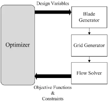
The optimization process developed in this study was implemented in SIMULIA Isight 5.7 commercial optimization software. Isight provides a common platform to link different programs required in the optimization process. Furthermore, several gradient and non gradient-based optimization strategies are embedded in Isight. Figure 3.1 presents the flowchart of aerodynamic optimization method developed in this study. The different elements of this flowchart will be explained in this chapter.

Figure 3.1 Flowchart of automatic design optimization

3.1 Reference blade

In this study NASA rotor 67 (see Figure 3.2) which is a transonic axial-flow fan rotor is used as the reference blade. This rotor is the first stage of a two-stage fan and was designed in the late 1980’s at the NASA Lewis Research Center (now Glenn). NASA rotor 67 has been a popular test case in many turbomachinery design optimization methods [38-41]. The experimental data for operating conditions at near peak efficiency and near stall is available in Ref. [42]. Table 3.1 presents the design characteristics of this rotor.

(37)

Figure 3.2 NASA rotor 67 [42]

Table 3.1 Design specifications of NASA rotor 67 [42]

Design pressure ratio 1.63

Design mass flow 33.25 kg/s

Design rotational speed 16 043 rpm

Tip speed 429 m/s

Inlet tip relative Mach number 1.38

Number of blades 22

Tip clearance 0.1016 cm

Aspect ratio (based on average span/root axial chord) 1.56

Rotor solidity 3.11 at the hub, 1.29 at the tip

Inlet tip diameter 51.4 cm

Exit tip diameter 48.5 cm

Inlet hub/tip radius ratio 0.375

(38)

3.2 Blade parameterization

Shape parameterization is one of the main challenges in an automatic optimization. Ideally, a parameterization should provide a low number of controlling parameters while maintaining the freedom to generate different shapes. Moreover, when used in an optimization, the parameterization needs to be robust to prevent the creation of irregular geometries. In this project, a three-dimensional fan blade parameterization method developed by Lupien [3] is used. This parameterization which is developed as a Matlab code has several unique features that make it valuable in an automated turbomachinery design. This section provides a brief overview of these features.

The starting point of Lupien’s work is a traditional approach to fan blade design which is based on quasi-3D analysis of 2D sections stacked along the span [43]. This method allows the designers to control the flow characteristics along the streamlines by manipulating the 2D sections. To achieve the desired flow around the 2D sections, designers use blade angles and slopes since these parameters are directly linked with flow characteristics of turbomachinery blades. However, due to the complexity of new designed blades, several sections are necessary to thoroughly define a blade. This leads to a large increase in the number of the design parameters. Furthermore, in traditional methods 2D sections are independently parameterized; thus, modifying a section may lead to an inconsistency in the overall shape of the blade. The method developed by Lupien maintains the advantages of traditional approach while significantly reducing the number of parameters required to define a blade. Moreover, this method provides a control on the blade geometry in the spanwise direction in order to prevent any inconsistency.

In Lupien’s geometry software, each 2D section airfoil consists of four parts: suction side, pressure side, leading edge, and trailing edge. The suction side is parameterized using the distributions of β-angle (angle between the tangent of the curve and the meridional direction) and its derivative (with respect to curvature) along the meridional chord. These distributions are defined by a set of control points which are connected by third-order polynomial curves. Typically, three control points are sufficient to define thin and not highly curved airfoil sections such as transonic fan blade profiles. The pressure side is then created by applying an offset from the suction side. The value of this offset at each chordwise location is extracted from a third-order polynomial which defines the distribution of thickness. This polynomial curve is constructed

(39)

using a set of control points for thickness and its derivative with respect to curvature. As for β-angle, typically three to five control points are needed to define the thickness distribution. The leading edge and trailing edge are then added to close the 2D section such that tangent continuity condition is satisfied at the junctions. For NASA rotor 67 circular arcs are used to create the leading edge and the trailing edge. The last step in the creation of a 2D section is the position of each section in the tangential direction (θ parameter). As it was mentioned earlier, the same control of design parameters is added in spanwise direction such that the distribution of each parameter is also defined by set a of control points which are used to generate B-spline curves. This spanwise control is the fundamental principle of this parameterization and arises from a natural continuity in the distribution of the parameters in spanwise direction of fan blades [3]. Figure 3.3 shows the 3D representation of the distribution of β-angle and thickness for NASA rotor 67.

Lupien’s software also provides a multi-level module for modifying the blade shape. This module is particularly beneficial in an automatic shape optimization process because it allows smooth modification of parameter distributions locally and globally. Moreover, this module reduces significantly the number of design parameters in an optimization process. To give an example, NASA rotor 67 is defined by 286 parameters using Lupien’s software; however, much less parameters are needed for its optimization. Figure 3.4 shows an example of applying multi-level module on β-angle distribution. It can be seen that the modification applied at 30% of span is propagated smoothly to the rest of the distribution curve. Several modifications at different spanwise location may be applied on a design parameter. In this case, the final spanwise distribution of this parameter is the summation of modified distribution curves.

As Cumpsty [17] showed, incidence angle has a strong impact on aerodynamic losses. Therefore, in the current study only β-angles and their derivatives were selected as design variables. Thickness is mainly important in structural design of fan rotors since reducing thickness has a significant effect on the stress level. Thus, thickness has been considered in structural design of MDO project. Table 3.2 presents the list of design variables and their bounds. Note that the design variables are the modification that we aim to apply on the design parameters of the reference blade. The left and right derivatives of β-angle at mid-chord section are imposed to be equal in this study in order to maintain the curvature continuity condition on the suction side.

(40)

Figure 3.3 Distribution of β-angle (Left) and Thickness (Right) in axial and spanwise directions [3]

Figure 3.4 Application of multi-level module Modification at

(41)

Table 3.2 Design variables and their bounds

Design variable Sign Bound

Modification on β angle at LE at hub [-3° to 3°]

Modification on β angle at LE at tip [-3° to 3°]

Modification on β angle at mid-chord section at hub [-3° to 3°] Modification on β angle at mid-chord section at tip [-3° to 3°]

Modification on β angle at TE at hub [-3° to 3°]

Modification on β angle at TE at tip [-3° to 3°]

Modification on right and left derivative of β at mid-chord section at hub

[-0.1 to 0.1]

Modification on right and left derivative of β at mid-chord section at tip

[-0.1 to 0.1]

Modification on right derivative of β at TE at hub [-0.1 to 0.1] Modification on right derivative of β at TE at tip [-0.1 to 0.1]

3.3 CFD simulation

The flow simulation was performed in Ansys CFX 14.5, a commercial package widely used in the turbomachinery industry and recommended by our industrial partner Pratt & Whitney Canada. Ansys CFX solves 3D Reynolds-Averaged Navier-Stokes (RANS) equations (time-average) using cell-vertex finite volume, coupled implicit, pressure based method.

Several turbulence models such as k-ε, k-ω and Shear Stress Transport (SST) are provided in Ansys CFX. SST is applied as turbulence model in this research. This model combines the advantages of both the standard k-ε and the k-ω models. At near wall region it employs the k-ω model to obtain more accuracy, while away from the wall it switches to the standard k-ε model to accelerate the calculations and obtain a more accurate solution. Furthermore, the SST model is designed to give highly accurate predictions of the onset and the amount of flow separation under

(42)

adverse pressure gradients. This is especially beneficial in modeling near stall flow separations [44].

Since in high speed flows the kinetic energy effects are important, total energy equation is solved to predict the temperature throughout the flow. The energy and momentum equations are coupled using the ideal gas model.

Defining boundary conditions and simulation setup

Figure 3.5 presents the computational domain and the boundary conditions. A single blade passage is simulated using a circumferential periodic boundary condition at the lateral boundaries. The inlet and outlet of the domain are both defined in the stationary frame and more than one blade pitch away from the leading edge and the trailing edge respectively to ensure that the perturbations of the flow around the blade do not affect the flow at these boundaries. At the inlet, total temperature and total pressure boundary conditions are imposed, and the flow direction is set to be normal to the boundary. At the outlet, a corrected mass flow rate as defined in Eq. (3.1) is assigned. In this equation, is the exit corrected mass flow at the desired operating condition. Moreover, and are standard pressure (101325 Pa) and temperature (288.15 K) at sea level.

(3.1)

The blade, hub and shroud are all defined in the rotating frame and the shroud is taken as a counter rotating wall. No-slip boundary condition is imposed on all solid surfaces, and the walls are assumed to be smooth.

(43)

3.4 Mesh selection

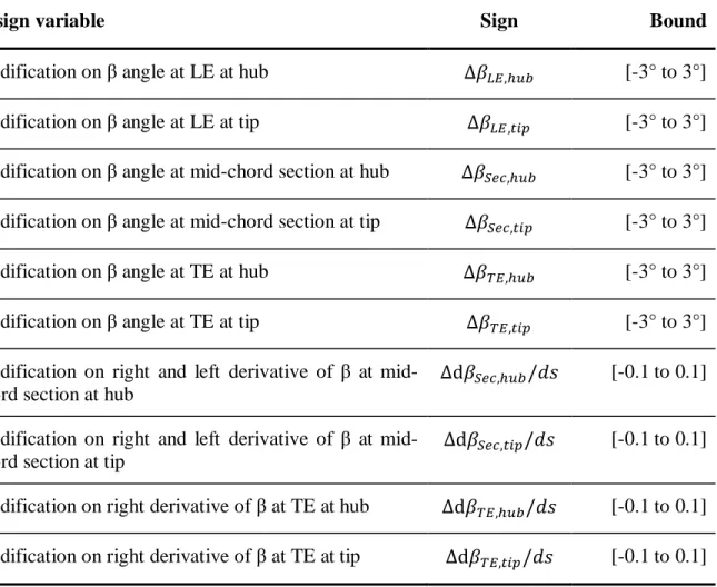
Ansys Turbogrid 14.5 is used in this project to create the mesh. A macro was developed to automate the entire process of mesh creation. A structured grid with H/J/C/L-Grid method including O-Grid type was created for the baseline blade considering the tip clearance. H/J/C/L-Grid allows for separate topology types in the upstream and downstream of the domain. This method is particularly beneficial in the simulation of transonic rotor blades where the mesh grid must be fine in the region close to the leading edge in order to capture the shock in this area. The size of the mesh in boundary layer is controlled by the value of y+, which is set to 1. This value for y+ is chosen with regard to the Reynolds number of the main flow, which is around 1e+6. To benefit from SST turbulence model, Ansys [44] recommends using at least 10 nodes in the boundary layer; 15 nodes are used in this study. Figure 3.6 shows the mesh independency study that is performed by increasing the overall number of nodes. Based on this study, the mesh with 1.2 million elements is selected to perform CFD simulations. This mesh grid contains 144, 78 and 100 elements in axialwise, pitchwise, and spanwise directions, respectively. Moreover, in order to accurately capture the effect of tip clearance flow, 20 elements are used in the tip gap. The computational grid is shown in Figure 3.7. The trends of y+ for this mesh in streamwise direction at 10%, 50% and 90% of span is presented in Figure 3.8.

Figure 3.6 Mesh independency study

89 89.5 90 90.5 91 91.5 0 1000000 2000000 Is en tr op ic e ffi c ie n c y (% ) Number of elements 150000 elements 1.6 1.61 1.62 1.63 1.64 1.65 0 1000000 2000000 P r e ss u r e r ati o Number of elements

(44)

(a) Blade grid (b) Hub-to-tip grid

(c) Blade-to-blade grid at 50% span Figure 3.7 Computational grid

(45)

(a) At 10% span (b) At 50% span

(c) At 90% span

Figure 3.8 Trend for streamwise y+ at (a) 10% (b) 50% (c) 90% of span

0 1 2 3 0 0.2 0.4 0.6 0.8 1 Y P lu s Chord fraction 0 1 2 3 4 5 0 0.2 0.4 0.6 0.8 1 Y P lu s Chord fraction 0 1 2 3 4 5 6 7 8 0 0.2 0.4 0.6 0.8 1 Y P lu s Chord fraction