Determination of phenological dates in boreal regions using Normalized Difference Water Index

(1)

HAL Id: ird-00392489

https://hal.ird.fr/ird-00392489

Submitted on 8 Jun 2009

HAL is a multi-disciplinary open access

archive for the deposit and dissemination of sci-entific research documents, whether they are pub-lished or not. The documents may come from teaching and research institutions in France or abroad, or from public or private research centers.

L’archive ouverte pluridisciplinaire HAL, est destinée au dépôt et à la diffusion de documents scientifiques de niveau recherche, publiés ou non, émanant des établissements d’enseignement et de recherche français ou étrangers, des laboratoires publics ou privés.

Determination of phenological dates in boreal regions

using Normalized Difference Water Index

Nicolas Delbart, L. Kergoat, Thuy Le Toan, J. Lhermitte, Ghislain Picard

To cite this version:

Nicolas Delbart, L. Kergoat, Thuy Le Toan, J. Lhermitte, Ghislain Picard. Determination of phenolog-ical dates in boreal regions using Normalized Difference Water Index. Remote Sensing of Environment, Elsevier, 2005, 97 (1), pp.26-38. �ird-00392489�

(2)

Editorial Manager(tm) for Remote Sensing of Environment Manuscript Draft

Manuscript Number: RSE-D-04-00841R2

Title: Determination of phenological dates in boreal regions using Normalized Difference Water Index

Article Type: Full length article

Section/Category:

Keywords: phenology; greening-up; senescence; NDWI; short-wave infrared; boreal; Siberia; SPOT-VEGETATION

Corresponding Author: Mr Nicolas Delbart,

Corresponding Author's Institution: Centre d'Etudes Spatiales de la Biosphère [CNRS-CNES-UPS-IRD]

First Author: Nicolas Jean-Paul Delbart

Order of Authors: Nicolas Jean-Paul Delbart; Laurent Kergoat; Thuy Le Toan; Julien Lhermitte; Ghislain Picard

(3)

Determination of phenological dates in boreal regions using Normalized

Difference Water Index

Nicolas Jean-Paul Delbart1_{, Laurent Kergoat}1_{, Thuy Le Toan}1_{, Julien Lhermitte}1_{, Ghislain Picard}2

1_{Centre d'Etudes Spatiales de la Biosphère [CNRS-CNES-UPS-IRD]}

2 _{Centre for Terrestrial Carbon Dynamics, Sheffield Centre for Earth Observation Science, University of Sheffield,} United Kingdom

ABSTRACT

Monitoring and understanding plant phenology is important in the context of studies of terrestrial productivity and global change. Vegetation phenology such as dates of onsets of greening up and leaf senescence have been determined by remote sensing using mainly the Normalized Difference Vegetation Index (NDVI). In boreal regions, the results suffer from significant uncertainties because of the effect of snow on NDVI. In this paper, SPOT VEGETATION S10 data over Siberia have been analysed to define a more appropriate method. The analysis of time series of NDVI, Normalized Difference Snow Index (NDSI) and Normalized Difference Water Index (NDWI), together with an analysis of in situ phenological records in Siberia, shows that the vegetation phenology can be detected using NDWI, with small effect of snow. In Spring, the date of onset of greening up is taken as the date at which NDWI starts increasing, since NDWI decreases with snowmelt and increases with greening up. In the Fall, the date of onset of leaf coloring is taken as the date at which NDWI starts decreasing, since NDWI decreases with senescence and increases with snow accumulation. The results are compared to the results obtained using NDVI-based methods, taking in situ phenological records as the reference. NDWI gives better estimations of the start of greening up than NDVI (reduced RMSE, bias and dispersions, and higher correlation), whereas it does not improve the determination of the start of

(4)

leaf coloring. A map of greening up dates in central Siberia obtained from NDWI is shown for year 2002 and the reliability of the method is discussed.

(5)

Introduction

Monitoring and understanding plant phenology, which is the timing of recurrent biological events, is gaining importance in the context of global change. Because of the long-term interest by biologists in phenology, many long time series of in situ phenological records exist, for example from meteorological stations or from “phenological gardens”. However, spatially and temporally continuous observations of phenology, required to study the effects of climatic changes on plant phenology, are difficult to generate from sparse ground stations. Consequently such observations have been derived from remote sensing data, especially from the Normalized Difference Vegetation Index (NDVI), an indicator of the density of chlorophyll and leaf tissue (Tucker et al., 1985) calculated from the red and near-infrared reflectances from the Advanced Very High Resolution Radiometer (AVHRR). NDVI temporal variations are related to the seasonal changes in the amount of photosynthetic tissues: for typical mid-to-high latitude ecosystems, NDVI increases when the deciduous vegetation greens up in spring and decreases when the vegetation changes color in autumn. Based on these variations, various algorithms have been applied to derive phenological dates from NDVI in previous studies (Justice et al., 1985, Reed et al., 1994, Lüdeke et al., 1996, Moulin et al., 1997, White et al., 1997, Duchemin et al., 1999).

Studies using AVHRR NDVI have shown that at northern latitudes the onset of greening up progressively earlier by a few days since 1982 (Myneni et al., 1997, Tucker et al. 2001, Zhou et al. 2001, Shabanov et al., 2002). This important result is in agreement with the lengthening of the growing season predicted by phenology models (Schwartz 1998) and observed in phenological

(6)

garden records (Menzel, 2000), and with the earlier onset of photosynthesis detected in the atmospheric CO2 concentration measurements (Keeling et al., 1996, Randerson et al., 1999).

However, detecting the onset of vegetation greening up from NDVI in boreal regions is difficult as the onset of NDVI increase corresponds to the beginning of snowmelt (Moulin et al., 1997). Shabanov et al.(2002) have analysed the time evolution of red and near-infrared reflectances in northern Europe during spring months from 1981 to 1991, and concluded that the trend observed from NDVI is not related only to an earlier vegetation onset of greening up but also to a reduction in the snow cover extent, which agrees with observations made by Dye and Tucker (2003).

Consequently, the effect of snow on the optical remote sensing data - in general NDVI of a given pixel increases when the snow cover fraction in the pixel decreases, and decreases when this fraction increases - must be taken into account when estimating the phenological dates in northern latitudes. To reduce the effects of snow on the NDVI signal, several solutions were proposed. Suzuki et al. (2003) define the onset of greening up as the first date of the year when NDVI exceeds a fixed threshold selected to be higher than NDVI of snow. Shabanov et al. (2002) derive greening up dates only on snow free areas. Zhang et al.(2003) replaces the vegetation index value by the last snow free record if snow is detected using a snow spectral index. Then, the date of onset of greening up is the date at which the modified vegetation index starts increasing.

Thanks to the spectral bands available on the recent optical sensors SPOT-VEGETATION (SPOT-VGT) and MODIS, other spectral indices can be calculated and should allow better

(7)

detection of phenological dates in Northern latitudes. In particular, two interesting spectral indices are:

− the Normalized Difference Snow Index (NDSI), a combination of blue and middle infrared bands (Hall et al., 1995) which is an indicator of the snow cover (Salomonson & Appel 2004),

− the Normalised Difference Water Index (NDWI), a combination of middle infrared and near infrared bands introduced by Gao to assess the water content of vegetation (Gao, 1996). NDWI has been used to monitor water stress in semi-arid environment (Fensholt, 2003), to map burnt areas in boreal forest (Fraser and Li, 2002), and to characterise land cover and vegetation type (Xiao et al., 2002 and Boles et al.,2004). The latter two papers mentioned the potential of this index for phenological date assessment. Boles et al. (2004) suggested also that the NDWI decrease preceding the increase due to vegetation development was due to snowmelt. Similarly, the authors suggested that the NDWI increase after senescence was due to snow accumulation.

The aim of this paper is to develop a method using NDWI to derive greening up and leaf coloring dates in boreal regions and to compare the results with those obtained using existing methods based on NDVI. In section 1, we describe the study area located in Central Siberia, the

in situ records (dates of beginning of snowmelt and snow cover formation, tree leaf appearance

and tree leaf senescence), and the remote sensing data which includes indices derived from SPOT-VGT S10 data. In section 2, we analyse the temporal variations of NDVI, NDSI and NDWI from 1999 to 2002. Together with the in situ records, the variations of NDSI are used to

(8)

identify the amount of NDVI and NDWI variations due to snow cover variations, and indirectly the part of these variations due to vegetation changes.

A method to estimate the dates of onsets of greening up and leaf coloring from NDWI is developed and described in section 3. Other existing methods using NDVI are described and applied to our datasets to derive the phenological dates. Section 4 presents the comparison between the dates obtained by remote sensing and the in situ observations. The reliability of each method and their ability to detect spatial and temporal phenological variations are assessed. Finally, the greening up date using NDWI is mapped in Siberia for 2002.

1 Study area and data

1.1 Study area

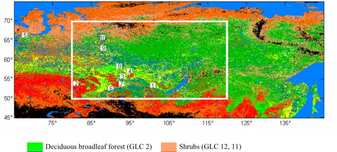
The study area ranges from 80°E to 120°E, and from 50°N to 70°N in Central Siberia (Fig. 1). The area is intensively studied in the SIBERIA-II project (http://www.siberia2.uni-jena.de/), which aims at fully accounting the carbon budget of vegetation and the greenhouse gas exchanges with the atmosphere, by means of multi-sensor remote sensing and vegetation modelling.

Climate in central Siberia is continental, characterised by very low temperatures in winter and a long snow period, typically from September to May. The main vegetation types include tundra in the North and in mountainous areas, taiga between latitudes 55°N and 65°N, and steppe, croplands and temperate forest in the South. Table 1 gives the area proportions for each cover type according to the Global Land Cover map GLC 2000 (Fritz et al., 2003). The main tree species in the taiga belt belong to the following genus : Larch (Larix), including Siberian Larch

(9)

(L. siberica), Spruce (Picea), Pine (Pinus) including Siberian Pine (P. sibirica) and Scot Pine (P.

silvestris), Birch (Betula), and Poplar (Populus).

1.2 In situ data

Phenological data used in this paper have been compiled by the Komarov Botanical Institute, Saint Petersburg. Russian phenological data originate from various networks, such as hydrometeorological stations, agriculture stations and nature reserves (Fedotova, 2000). Methodologies for phenological observations are described in Bulygin (1976) and Elagin (1975). The records include the dates of leaf appearance and autumn leaf coloring for birch, aspen and larch, the dates of snow events such as beginning of snowmelt and beginning of snow cover formation, all obtained through visual observations. One record set dates back to 1902, but many were from more recent years (table 2). All records, from sites 1 to 10 are used for the analysis, whereas only records from sites 1 to 5 are used for validation of remote sensing methods.

1.3 Remote Sensing data

SPOT-VGT 10-day-composite data (S10) at the resolution of 0.008928° (about 1km) in plate-carree projection were downloaded (http://free.vgt.vito.be/). Data consist in reflectances in spectral bands B0, B2, B3 and SWIR, which correspond respectively to the blue (0.43-0.47µm), red (0.61-0.68 µm), near-infrared (0.78-0.89 µm) and short-wave infrared (1.58-1.75 µm) domains. These reflectances are combined to calculate NDVI, NDWI and NDSI as:

NDVI= (B3-B2)/(B3+B2) (1),

(10)

NDSI=(B0-SWIR)/(B0+SWIR) (3).

For each pixel, one acquisition – i.e. one reflectance value for each spectral band- is selected for each 10-day period, based on a Maximum Value Composite (MVC) technique (Holben, 1986). The selected acquisition is expected to be the least affected by atmospheric disturbances. The exact acquisition date is provided in the dataset. Duration between two consecutive S10 data ranges from 1 to 20 days.

Despite MVC procedure, S10 data may still be affected by clouds and aerosols. Aerosols affect more strongly the shortest wavelengths (B0, B2) signals. Therefore, NDSI is more sensitive to aerosols than NDVI, which is more sensitive than NDWI.

2 Data analysis

2.1 In situ data

For each of the 10 sites, table 3 summarises the mean, standard deviation and temporal range of the key phenological and snow dates. Means and standard deviations of the time intervals between events are also reported. The standard deviation refers to interannual variation, and not to the uncertainties in the in situ observations which are difficult to estimate since they depend significantly on the observers.

2.1.1 Spring events

In all the records, first leaves appear after the beginning of snowmelt (column 6 in table 3). The time interval between the beginning of snowmelt and the appearance of first leaves is of the order of 34 days, and shows significant interannual variations (standard deviation of 17 days on average). Interannual variations of the snowmelt date (column 5) are larger than those of leaf

(11)

For every site, leaf appearance dates for the different deciduous species are close. In particular birch and larch show a very similar phenology in spring (column 3), with no difference on average (all sites and all years averaged). The average time difference between birch and aspen (column 4) is 3 days (std 4.7). Such a high uniformity of phenological events is also pointed out by Linkosalo (1999) for Finnish forests, and ascribed to similar responses of trees to climate conditions. The spatial gradient is 34 days in average between the most Southern and Northern sites, whereas at each site mean interannual variabilitions are about 30 days.

2.1.2 Autumn events

The various species start their foliage senescence at various times. In general, aspen starts coloring earlier than birch, followed by larch (not shown in table 3). The time interval between the senescence of the various species is not constant. For example it ranges from 0 to 40 days between aspen and larch for the years under study. In addition, for a given species at a given site, the interannual variabilitions are large: for example, the beginning of birch senescence varies from –20 days to 20 days around the average date. In general, the senescence starts before the first snowfall. However, larch trees start their senescence quite often after the formation of the permanent snow cover.

2.2 Analysis of spectral indices from SPOT-VGT

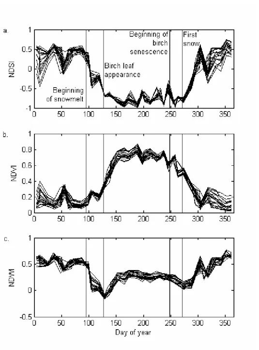
Fig. 2 and 3 show typical variations of the three spectral indices in relation with the phenological and snow events. They outline the logic of the algorithm, which is developed in section 3. Fig. 2 presents the 1999 time series of NDSI, NDVI and NDWI for deciduous forest pixels near

(12)

Krasnoyarsk, a southern site of the study area, with the in situ dates of snowmelt, appearance of birch leaves, beginning of coloring of birch leaves and the beginning of the snow cover formation. Fig. 3 presents the 2000 time series of the three indices for larch pixels near Aksarka, a northern site, with the dates of beginning of snowmelt and first appearance of larch needles. At the resolution of VGT data, a pixel contains a mixture of snow, green vegetation and non vegetated areas. When applied to optical data, the term snowmelt corresponds to the decay of the area covered by snow in the pixel, while the vegetation greening up corresponds to the increase of the area of green vegetation in the pixel. In autumn, leaf coloring corresponds to the increase of the area of yellow or brown vegetation in the pixel. Last, snow cover formation corresponds to the increase of the snow-covered area in the pixel.

2.2.1 Spring events

In Fig. 2 and 3 NDSI starts decreasing at the beginning of snowmelt. This decrease either continues until or after the appearance of leaves (Fig. 2), until complete snow disappearance, or ends before leaf appearance(Fig. 3) if snowmelt ends before leaf appearance. As expected, NDSI exhibits large variations during summer, due to atmospheric effects.

NDVI increases as the proportion of green leaves increases in the pixel, and is close to zero for a pixel covered by snow. Thus, NDVI increases during both snowmelt and leaf appearance, resulting in either one continuous increase (Fig. 2), or in two distinct increases if snowmelt ends before the leaf appearance (Fig. 3). In the first case, the two events can not be distinguished in the NDVI time series. In the second case, the distinction is difficult since there is no significant change such as a change in the sign of the slope.

(13)

NDWI is related to the quantity of water per unit area in the canopy (Gao, 1996). It therefore increases during leaf development. However, as opposed to NDVI, it decreases during snowmelt (Boles et al., 2004). NDSI time series show that greening up may start before or after complete snowmelt. If snowmelt did not melt totally well before leaf appearance (one week or more), NDWI first decreases and then increases (Fig. 2), displaying a “peak” at its minimum. If snowmelt is complete before leaf appearance, then NDWI remains stable during a period which may last between a few days to a few weeks before increasing (Fig. 3).

If greening up occurs during snowmelt, the NDWI decrease due to snowmelt may mask the NDWI increase due to greening up, and NDWI may start increasing later than the actual onset of greening up. However, in situ records show that snowmelt starts in average several weeks before greening up. Thus, in the majority of the cases, a large proportion of snow cover has already melt at the onset of greening up, and the moment at which NDWI starts increasing corresponds to the onset of greening up.

2.2.2 Autumn events

As illustrated in Fig.2, NDSI remains stable during vegetation coloring, and increases during the formation of the snow cover. NDVI decreases both during vegetation coloring and snow cover formation, and shows only a single and continuous decrease. It is difficult to ascribe specific portions of such a decrease to one or the other event.

NDWI decreases during vegetation coloring. The slow increase in NDWI after the first snow (e.g. on day 270 in Fig. 2c) can be interpreted in two ways:

(14)

− the snow cover formation is slow at the beginning,

− there is compensation between the NDWI decrease due to vegetation coloring and the NDWI increase due to snow. In some cases (not shown in Fig. 2 and 3), NDWI does not decrease at all during autumn, which indicates that snowfalls start before or at the beginning of vegetation coloring.

3 Algorithm development

3.1 Assessment of noise and data filtering

The noise due to atmosphere and to the sensor must be taken into account in our detection algorithm, and is quantified in this section. For this purpose, we study the temporal variations of the three indices at the end of July when changes due to phenology and snow are expected to be minimum. The distributions of the variations of the three indices between the last two 10-day periods of July are computed. For the three indices, the mean is close to zero, and the standard deviations, which are subsequently considered as noise level, are 0.06 for NDVI, 0.1 for NDSI, and 0.03 for NDWI. Additionally, we assume that the variations due to noise in late spring are the same as those in July.

The MVC processing retain data contaminated by clouds or high aerosol loading if all data within the 10-day period are affected. For the late spring and summer period, the data are filtered out using a threshold of 0.4 on NDSI positive variations between consecutive 10-day periods. Autumn data were not filtered because successive snow falls and snowmelts have the same signature on NDSI than clouds and aerosols.

(15)

3.2 Estimation of the date of onset of greening-up

Following the above analysis, a method using NDWI is developed to extract the date of onset of vegetation greening up. For comparison purposes, the dates of onset of greening up are computed by applying three existing methods using NDVI.

3.2.1 Methodology for NDWI time series

During the spring, minimum NDWI corresponds to the vegetation state before greening up. It can be used to detect the onset of vegetation greening up, except if there is a plateau between snowmelt and vegetation greening up, as described in section 2.2.1. In this case, small fluctuations of the NDWI may arbitrarily position the minimum in the plateau period, causing a mismatch between minimum NDWI and the onset of vegetation greening up. Therefore, our algorithm retains the later NDWI record which is less than the minimum NDWI increased by an estimate of the noise level (Fig. 4a and 4b, and eq. 4). In addition for these boreal ecosystems, we assumed that onset of greening up must occur prior to day-of-year 200 (18th-19th July).

[

]

(

)

(

∈ < +ε

)

=maxt 0,200 NDWI(t) NDWImin

t_greening (4)

εwas chosen to fulfill the following constraints :

− ε should be larger than the noise affecting NDWI time profile.

− εmust be smaller than the first NDWI increase due to vegetation growth.

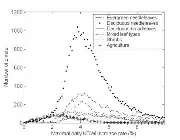
To assess this increase, statistics of NDWI increase following the minimum NDWI are analysed. For all the pixels of the study area, the daily rate of increase is calculated for the three 10-day periods following the minimum NDWI. In 80% of non-agricultural pixels, the maximum rate occurs during the first or the second 10-day period after the minimum NDWI. This means that the increase is rapid as soon as it starts. The distribution of the maximum rate for different forest

(16)

and cover types is shown in Fig. 5. When expressed as a percentage of the overall spring NDWI increase (hereafter referred to as NDWI amplitude), the average rate is 4% per day, except for some agricultural areas. Finally, either the first or the second 10-day period of increase accounts on average for 40% of the amplitude. Such a value appears to be an upper limit for ε.

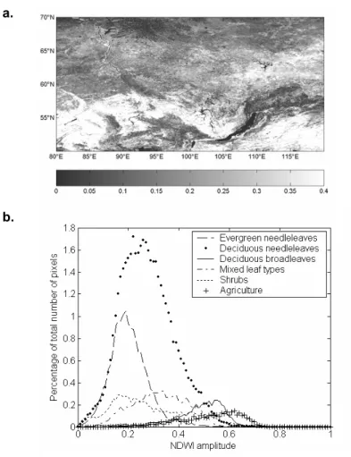
Based on these considerations, ε was chosen to be 20% of the spring NDWI amplitude. For pixels displaying an amplitude of 0.2 or more (71% of all pixels, see amplitude map in Fig. 6a and its distribution by land cover in Fig. 6b), this means that the detection is not affected by noise induced variations up to 0.04, which is above the estimated standard deviation of noise (estimated as 0.03 NDWI units, see section 3.1). Only 4% of non-agricultural pixels have a maximum increase rate lower than 2% of spring amplitude. For these pixels, there is a siginificant risk to overestimate the date of onset of greening up by one 10-day period or more.

3.2.2 Methodologies for NDVI time series

Several methods have been used to detect the onset of greening up from vegetation index data (Lloyd 1990, Reed et al. 1994, Moulin et al. 1997, White et al. 1997, Schwartz et al. 2002, Zhang et al. 2003, Suzuki et al. 2003 among other). Among them, two methods were selected and applied to our data. The first method relies on the detection of the beginning of NDVI increase. Two variants of this method are tested (methods 1a and 1b). In the second method, the onset of greening up is defined as the date NDVI exceeds a threshold. The threshold is either pixel dependant (method 2a), or spatially uniform (method 2b).

(17)

Method 1a was developed by Zhang et al. (2003, 2004) to detect spatial variations of phenological dates from the Enhanced Vegetation Index (Huete et al., 2002) calculated from the MODIS nadir BRDF-adjusted reflectances (NBAR) for latitudes higher than 35°N. We apply it on the NDVI time series. It consists in fitting logistic functions y(t) to the NDVI time series. y(t) is defined by: d bt a e c t y ₊ + + = ) ( 1 ) ( (5)

where a and b are fitted coefficients linked to temporal variations of NDVI, c+d is the maximum NDVI value and d the minimum NDVI value. Two distinct functions are fitted for the greening up and the leaf coloring. Since the phenological cycle may be multimodal, local extrema are detected using a polynomial fit (9th order) in order to select the main mode. The onset of the NDVI increase is then taken as the date of maximum positive curvature of the ascending function.

In Zhang et al. (2004), EVI data for which snow is detected (using MODIS quality assurance flags and MODIS Land Surface Temperature) are replaced by snow free data. In this paper, we use a variant of this method to reduce the effect of snow accumulated on the canopy. We assume that the maximum NDVI between January and March (when deciduous species are leaf-less) corresponds to the minimum accumulation of snow on the canopy. NDVIs lower than this maximum are replaced by this maximum. Method 1a consists in estimating the date at which this modified NDVI starts increasing as defined above. Method 1b is the same applied to the non-modified NDVI.

(18)

In the threshold methods (Lloyd 1990, White et al. 1997, Schwartz et al., 2002, Suzuki et al. 2003), the onset of greening up is assumed to occur when NDVI exceeds a certain value. In White et al. (1997), the date of onset of greening up is defined as the day at which NDVI has increased by half its total amplitude. We modify this method in order to keep the strong noise removal induced by the fit of the logistic function as used in method 1b. Therefore method 2a consists in estimating the date at which the fitted function has increased by half its amplitude

In method 2b, the same threshold value is used for all the pixels. Suzuki et al. (2003) choose a value of 0.2 (AVHRR dataset) considering that a snow covered surface would have a lower NDVI. Since AVHRR NDVI and SPOT-VGT NDVI are not directly comparable due to differences in sensor spectral response, orbits and data processing, we retain the threshold on VGT NDVI, which gives the smaller bias with the in situ data (see section 4.1). This retained NDVI threshold is 0.4.

3.3 Extraction of leaf coloring onset date

Method for NDWI

We define the beginning of NDWI decay, which corresponds to leaf coloring or senescence, as the date for which NDWI has decayed by 20% of its autumnal amplitude (other quantities were tried with poorer results).

(19)

Following Zhang et al. (2003), a logistic function is fitted to the descending part of the NDVI time series. Senescence is defined as the start of NDVI decay, which is the date of minimum curvature (largest negative curvature value).

Method 2 for NDVI

Alternatively, senescence is estimated by the date for which the fitted NDVI has decayed by 20% of its autumnal amplitude. This method follows the threshold approach of White et al. (1997), although in their method no function is fitted to the data.

3.4 Methodology of validation

The greening up and senescence dates derived from remote sensing data are compared with in

situ data. To avoid mis-registration of in situ site and SPOT-VGT pixel, it is preferable to

compare the in situ dates to the dates averaged on pixels of the same vegetation type located in an area (window) surrounding the in situ site. This is justified by the fact that phenology is driven by climate, and thus does not display strong short–scale gradient. Different window sizes were tried, to obtain a good trade-off between a representative number of pixels corresponding to the in situ vegetation class, which favours larger windows, and the proximity to the in situ site, which favours small windows.

Finally the dates of onset of greening up dates using NDVI and NDWI for the deciduous forest pixels (GLC2000 classes 2, 5 and 6) in the window around each in situ measurement point, are compared to the average date of birch and larch leaf appearance (which are very close to each other, as shown in section 2.1) from 1999 to 2002.

(20)

Dates of onset of leaf coloring found on pixels of classes 2 and 6 (deciduous broadleaf and mixed forests) in the window are plotted against in situ dates of birch senescence. Dates found on pixels of class 5 (larch) are plotted against the in situ dates of larch senescence, as significant difference exist between the date of senescence of broadleaves and larch as shown in section 2.1.2.

The root mean square error (RMSE), bias, dispersion and correlation coefficient are calculated from all pixels and all years. Correlation coefficient is also calculated from the mean value of all pixels in one window. Formulations of RMSE, bias and dispersion as given in Willmott (1982) are given in eq. 6 to 8 :

N y x RMSE i N i i 2 ) ( − =

∑

(6), N y x Bias N i i i

∑

− = ) ( (7), and

∑

− − − = N i i i y Bias x N Dispersion ₍ ₎2 1 1 (8),

where xi is the date obtained by remote sensing, yi is the in situ date for a given pixel in a given year. N is the total number of pixels multiplied by the number of years.

(21)

4 Results

4.1 Greening-up

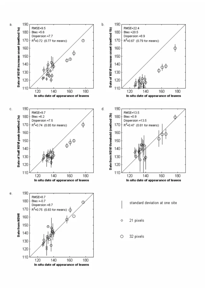
The comparison between retrieved greening up dates and in situ dates are presented in Fig. 7. Circles represent the mean value of the dates retrieved for the window around a given in situ site. They are plotted against the average in situ date of appearance of birch and larch leaves. Vertical lines represents the standard deviation. The size of the circles is proportional to the number of the corresponding pixels found in each window. The window size is 0.14° for sites 1, 2, 4 and 5, and 0.34° for site 3. This allows to have a number of deciduous forest pixels ranging from 21 to 32 for all sites, ensuring a balanced importance of all sites in the calculations.

Results from methods 1a and 1b are presented in Fig. 7a and 7b. The two methods display similar dispersion and correlation coefficients. However, the biases are different, being 19 days for method 1b, and 6 days for method 1a. This indicates that it is relevant to replace low NDVIs by the highest winter NDVI. For both methods, the bias is higher for the northernmost site, which shows leaf appearance dates later than day of year 150. In Zhang et al. (2004), snow detection is further completed using an additional filter based on MODIS Land Surface Temperature, which may further reduce the bias and the dispersion.

The results obtained with method 2a are similar to those obtained with method 1a. The bias is larger for the northernmost pixels, whereas in the southern taiga, the remote sensing estimates are relatively closer to the in situ measurements. As the method is based on the detection of the date of half-amplitude on the fitted logistic, the result seems to indicate that in these pixels, the first half of the NDVI increase is due to snowmelt whereas the second half is due to vegetation

(22)

greening up. However the amplitude proportions depend on land cover or latitude: in the North the half amplitude occurs earlier than the in situ leaf appearance, which occurs between days 155 and 180. This means that more than half of the NDVI increase is due to snowmelt for the Northern sites.

The dates obtained with the threshold method, NDVI method 2b, are highly dispersed, which means that the dates of onset of greening up can not be determined precisely. Interannual variations seem difficult to detect, because of the dispersion. However the bias is small, as we determined the threshold in order to minimize it, and is similar in the Northern and in the Southern sites. This suggests that North-South spatial gradients in the dates of greening up can be determined, as shown in Suzuki et al.(2003).

The best results are obtained with the NDWI method, for South and North sites. There is almost no bias with in situ measurements. The dispersion is much lower than with NDVI-method 2b. RMSE, bias and dispersion are also calculated year by year, providing values similar to their values calculated with all years. This shows that the spatial variability can be retrieved for any given year. Calculations are also made on each individual site (all years considered) to evaluate the ability of the method to retrieve interranual variations at a given site. At Krasnoyarsk, Taseevo and Aksarka (sites 3, 4 and 5), but not at Ilir (site 1), the correlation between the retrieved dates and the in situ dates is good, indicating that the interannual variations could be retrieved. Unfortunately the small amount of in situ data does not allow to firmly conclude on the robustness of the method to determine the interannual variations.

(23)

To assess the effect of the window size on the results, window sizes ranging from 0.06° to 0.36° were tested. Whatever the window size, the dates obtained with the NDWI method display the best overall statistics, with a RMSE ranging from 6.5 days to 9.5 days.

As a result, the determination of the date of onset of greening up using NDWI appears robust, due to the fact that the effects of snow and vegetation on NDWI are in opposite direction, combined with NDWI’s relative lack of sensitivity to aerosols.

4.2 Leaf coloring

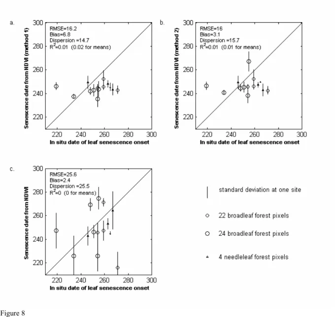
Fig. 8 shows the comparison of the date of onset of leaf coloring obtained using NDWI and NDVI methods 1 and 2 with in situ dates of beginning of senescence. Dates obtained for broadleaf pixels are compared to the in situ date of beginning of senescence of birch (circles), and dates obtained on larch pixels are compared to the in situ dates of beginning of senescence of larch (triangles). Window sizes are similar to those in 4.1.

The three methods using NDVI or NDWI give poor results, with low R2 and high RMSE (especially for NDWI-based method). Moreover, the spatial variations are not properly observed, as the retrieved dates in the North are very close to the dates in the South, whereas in situ data show significant differences. We examined in the following possible causes of such discrepancies.

− Because of the low amplitude of NDWI variations in autumn, the detection of the beginning of index decay may not be robust. The 20% of the variation amplitude may be too small to be detectable, but other threshold values were tested with even poorer results.

(24)

− Leaf senescence of different species and different trees start at different times. Thus, extracting a date of onset of leaf coloring for a pixel and comparing it to in situ senescence measurement for one species is not straightforward. Moreover, leaf senescence corresponds to various changes in chemical and structural properties, resulting in changes in spectral responses which may start long before leaf abscission. This is the opposite of spring phenology, where leaf appearance is much more well defined in time.

− The decrease in the water content observed by NDWI may not be linked to the decrease of the chlorophyll content detected by the in situ observations (Ceccato et al. 2001).

− The decrease in NDVI at the end of season “may be related to abiotic factors, such as extended period of cloudiness” (Reed et al., 1994).

In summary, contrary to the dates of onset of greening up, the dates of onset of leaf coloring retrieved from NDVI or NDWI are not accurate. In the following, only the dates of onset of greening up dates are mapped.

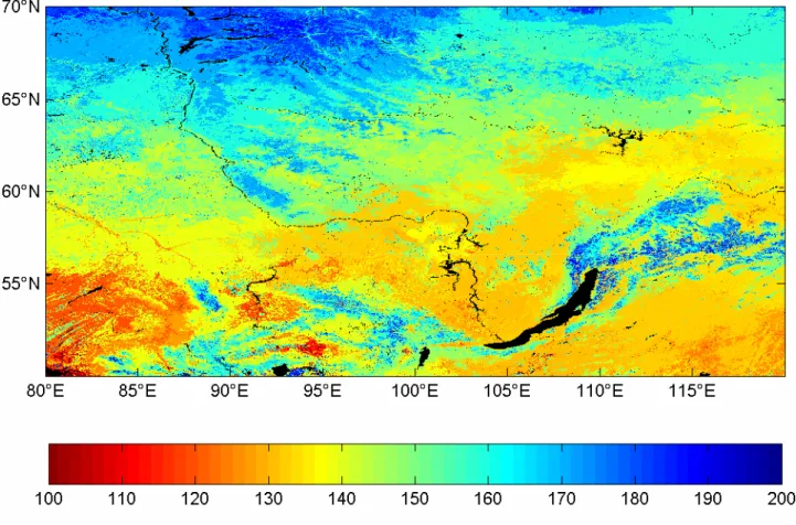
4.3 Map of greening up dates in Siberia

Fig. 9 shows the dates of onset of greening up obtained using NDWI in year 2002 for the study area represented by the rectangle in Fig. 1. The general pattern is a South to North gradient, with earlier onset of greening up in the South. The exception to the South-North gradient is found in regions corresponding to mountainous areas located in the North, in the North East of the Lake Baikal, and in the South of the area, which display later onset of greening up compared to areas at the same latitude.

(25)

4.4 Discussions

The dates of onset of greening up of forest pixels with a large proportion of deciduous trees or understorey vegetation are expected to have uncertainties similar to uncertainties represented by RMSE at validation sites. It is likely that a large part of these uncertainties come from the temporal resolution of the VGT S10 data.

In addition to the overall validation based on comparison with independent in situ data, different sources of error in the retrieval algorithms can be assessed:

1) Phenological dates are also calculated for agricultural pixels, although the 20% threshold used in the NDWI algorithm is not optimised for cropland, as NDWI variations show a different behaviour compared to forests (Fig. 5). The corresponding uncertainties are unknown, since no

in situ data for crops were available for validation.

2) The detection is dependent on the εvalue, which is a proportion of the NDWI increase amplitude in spring. When this amplitude is small, NDWI variations we want to detect are close to the variations due to noise. Fig. 6a shows that the amplitude is low in the three mountainous regions and in the tundra as expected, because of the small amount of vegetation, and also possibly because of the long period of overlap between snowmelt and vegetation greening. The estimated dates at these regions are thus likely to be more affected by noise and likely to be less accurate. Low amplitude is also found in pixels where the proportion of deciduous vegetation is small compared to the proportion of evergreen vegetation. Onset of greening up detection is therefore more uncertain in these regions. A land cover map with deciduous/evergreen proportion may be used to exclude pixels where the deciduous proportion is small. However for

(26)

all pixels where the amplitude is low, a flag corresponding to a higher level of uncertainty can be assigned directly based on the signal amplitude without any a priori information.

3) If snowmelt and greening up overlap during a long period, NDWI variations with snowmelt and greening up compensate, making NDWI start increasing later than the actual onset of greening up. However, no such case was found in our in situ records. Moreover, because of the compensation between the NDWI decrease and increase, the overall spring amplitude is low. Such pixels can consequently be assigned a higher level of uncertainty as described above.

4) Last, NDWI time series may be sensitive to water intercepted by leaves and to abrupt increase in soil moisture (Madeira et al. 2001, Xiao et al. 2002). Given the fact that our algorithm uses NDWI thresholds and does not retain isolated NDWI peaks, possible impacts of these effects on phenology are likely to be limited. The method may also be affected by short term land cover changes, such as floods or fires. Such effects can be removed by using flood and fire information, acquired independently.

Conclusion

In this paper, we have presented an alternative method to the use of NDVI to determine a key phenological date:the date of onset of greening up in the boreal regions. This method relies on the properties of NDWI, calculated from SPOT-VGT S10 data, which is similar to the NDVI but with the red band replaced by the short wave infrared band. NDWI decreases during snowmelt and increases during greening up, thus allowing distinction between snowmelt and vegetation greening up in spring, which is not possible with NDVI. The date of onset of greening up is taken as the date NDWI starts increasing in spring. The comparison with in situ phenological

(27)

records shows that NDWI is more efficient to estimate the date of onset of greening up than other methods based on NDVI in the Siberian context.

Estimating the date of onset of leaf coloring in autumn proved to be less satisfactory, for both NDVI and NDWI, since poor agreement was found with the in situ dates of beginning of leaf senescence. This result could be due either to the heterogeneity in the dates of beginning of tree senescence within a pixel, or to the complexity of leaf senescence process and associated changes in spectral responses, or to abiotic factors such as atmospheric effects. It may thus not be possible to accurately measure the length of the active period of boreal vegetation through the use of these indices.

The date of onset of greening up was mapped for year 2002 for an area located between 80° and 120° in longitude, and between 50° and 70° in latitude. The accuracy of spring phenology retrieval differs among pixels, as the quality of the determination of the date of onset of greening up depends on properties of each time series, like the spring amplitude and the rate of increase, which change the sensitivity of the detection to the residual noise.

One limitation is the use of 10-day composite data, which prevents the detection of fine variations. In the future, the method could be refined using VGT daily data in order to reduce the error linked to the temporal resolution of the S10 data. The method could also be applied to MODIS data (bands 2 and 6) at the 500 metre resolution.

For long time series however, a method needs to be developed to interpret the NOAA/AVHRR archive, with a focus on the removal of the effect of snow. Our results may help analysing AVHRR Pathfinder data to retrieve leaf appearance dates over the whole Siberia from 1982

(28)

onwards. The results could be used to calibrate or validate phenological models incorporated in the dynamic vegetation models (Botta et al., 2000), and to estimate the impact of phenological changes on terrestrial carbon budget (White, 2003).

Acknowledgements

Vegetation phenology data were provided by Dr. Violetta Fedotova, of the Phenology research group at the Institute of Botany, Komarov Russian Academy of Sciences, St. Petersburg.

This work was conducted in the framework of the Siberia II project ( Multi-sensor concepts for Greenhouse Gas Accounting of Northern Eurasia), EC Framework 4 Contract: EVG1-CT-2001-00048.

(29)

5 References

Boles, S.H., Xiao, X., Liu, J., Zhang, Q., Munktuya, S., Chen, S., & Ojima, D. (2004), Land cover characterization of Temperate East Asia, using multi-temporal VEGETATION sensor data, Remote Sensing of Environment, 90, 477-489.

Botta, A., Viovy, N., Ciais, P., Friedlingstein, P., and Monfray, P. (2000), A global prognostic scheme of leaf onset using satellite data, Global Change Biology, 6(7):709-725.

Bulygin, N. E. (1976). Dendrology. Phenological observations on deciduous trees. Leningrad: Leningrad Forest Technology Academy. 70 pp (in Russian).

Ceccato, P., Flasse, S., Tarantola, S., Jacquemoud, S., & Grégoire, J-M. (2001), Detecting vegetation leaf water content using reflectance in the optical domain, Remote Sensing of

Environment, 77, 22-23.

Duchemin, B., Goubier, J., & Courrier, G. (1999), Monitoring phenogical key stages and cycle duration of temperate deciduous forest ecosystems with NOAA/AVHRR data, Remote

Sensing of Environment, 67, 68-82.

Dye, D.G., & Tucker, C.J. (2003), Seasonality and trends of snow-cover, vegetation index, and temperature in Northern Eurasia, Geophysical Research Letters, 30(7), 1405, 58(1)-58(4). Elagin, I. N. (1975). Methodology for collecting and processing data of phenological

observations on trees and shrubs. In: I. N. Elagin, T. N. Bytorina, Editors Phenological

methods for studying the forest biocenoses (pp. 3-20). Institute of Forest and Wood of

Siberian Branch of Academy of Sciences of USSR, Krasnoyarsk. (in Russian)

Fedotova, V.G. (2000), Russian phenology: history and present day (poster), International

Conference : Progress in Phenology, Monitoring, Data Analysis, and Global Change Impacts, October 4-6, 2000, Freising, Germany.

Fensholt, R., Sandholt, I. (2003), Derivation of a shortwave infrared water stress index from MODIS near- and shortwave infrared data in a semiarid environment, Remote Sensing of

Fraser, R.H., Li, Z., Estimating fire-related parameters in boreal forest using SPOT VEGETATION, Remote Sensing of Environment, 82, 95-110.

Fritz, S., Bartholomé, E., Belward, A., Hartley, A., Stibig H., Eva, H., Mayaux, P., Bartalev, S., Latifovic, R., Kolmert, S., Sarathi Roy, P., Agrawal, S., Bingfang, W., Wenting, X.,

(30)

Ledwith, M., Pekel, J., Giri, C., Mücher, S., De Badts, E., Tateishi, R., Champeaux, J., & Defourny, P. (2003), The Global Land Cover for the Year 2000, Harmonisation,

mosaicing and production of the Global Land Cover 2000 database (Beta Version),

European Commission, Joint Research Centre, EUR 20849 EN.

Gao, B.C. (1996) NDWI – a normalized difference water index for remote sensing of vegetation liquid water from space, Remote Sensing of Environment, 58, 257-266.

Hall, D.K., Foster, J.L., Verbyla, D.L., Klein, A.G. & Benson, C.S. (1998): Assessment of snow-cover mapping accuracy in a variety of vegetation-snow-cover densities in central Alaska.

Remote Sensing of Environment 66, 129-137.

Holben, B.N. (1986), Characteristics of maximum-value composite images from temporal AVHRR data, International Journal of Remote Sensing, 7, 1417-1434.

Huete, A., Didan, K., Miura, T., & Rodriguez, E. (2002), Overview of the radimetric and biophysical performance of the MODIS vegetation indices, Remote Sensing of

Justice, C.O., Townshend, J.R.G., Holben, B.N., & Tucker, C. J. (1985), Analysis of the phenology of global vegetation using meteorological satellite data, International Journal

of Remote Sensing, 6, 1271-1318.

Keeling, CD, Chin, J.F.S., & Whorf, TP (1996) Increased activity of northern vegetation inferred from atmospheric CO2 measurements, Nature, 382, 146-149.

Linkosalo, T. (1999), Regularities and patterns in the spring phenology of some boreal trees,

Silva Fennica, 33(4), 237-245.

Lloyd, D. (1990), A phenological classification of terrestrial vegetation cover using shortwave vegetation index imagery. International Journal of Remote Sensing, 11, 2269-2279. Lüdeke, M.K.B., Ramge, P.H., & Kolhmaier, G.H. (1996), The use of satellite NDVI data for the

validation of global vegetation phenology models : application to the Frankfurt Biosphere Model, Ecological Modelling, 91, 255-270.

Madeira, A.C., Gillepsie, T.J., Duke, C.L. (2001), Effect of wetness on turfgrass canopy

reflectance, Agricultural and Forest Meteorology, 107, 117-130.

Menzel, A. (2000), Trends in phenological phases in Europe between 1951 and 1996,

(31)

Myneni, R.B., Keeling, C.D., Tucker, C.J., Asrar, G., & Nemani, R.R. (1997), Increased plant growth in the northern high latitudes from 1981 to 1991, Nature, 386, 698-702.

Moulin, S., Kergoat, L., Viovy, N., & Dedieu, G.(1997), Global-scale assessment of vegetation phenology using NOAA/AVHRR satellite measurements, Journal of Climate, 10, 1154-1170.

Randerson, J.T., Field, C.B., Yung, I.Y., & Tans, P.P (1999), Increases in early season ecosystem uptake explain recent changes in the seasonal cycle of atmospheric CO2 at high northern latitudes, Geophysical research letters, 26(17), 2765-2768.

Reed, B.C., Brown, J.F., VanderZee, D., Loveland, T.R., Merchant, J.W., & Ohlen, D.O.(1994), Measuring phenological variability from satellite imagery, Journal of Vegetation Science,

5, 703-714.

Salomonson, V.V., & Appel, I. (2004), Estimating fractional snow cover from MODIS using the normalized difference snow index, Remote Sensing of Environment, 89, 351-360.

Shabanov, N.V., Zhou, L., Knyazikhin, Y., Myneni, R.B., & Tucker, C.J.(2002), Analysis of interannual changes in northern Vegetation activity observed in AVHRR Data from 1981 to 1994, IEEE Transactions on Geoscience and remote sensing, 40(1), 115-130.

Schwartz, M.D. (1998), Green-wave phenology, Nature, 394, 839-840.

Schwartz, M.D., Reed, B.C., & White, M.A., (2002), Assessing satellite-derived start-of-season measures in the conterminous USA, International Journal of Climatology, 22, 1793-1805.

Suzuki, R., Nomaki, T., & Yasunari, T.(2003), West-east contrast of phenology and climate in northern Asia reavealed using a remotely sensed vegetation index, International Journal

Biometeorology, 47, 126-138.

Tucker, C.J., Townshend, J.R.G., & Goff, T.E. (1985), African land-cover classification using satellite data, Science, 227(4685), 369-375.

Tucker, C.J., Slayback, D.A., Pinzon, J.E., Los, S.O., Myneni, R.B., & Taylor, M.G (2001), Higher northern latitude normalized difference vegetation index and growing season trends from 1982 to 1999, International Journal of Biometeorology, 45, 184-190.

White, M.A., Thornton, P.E., & Running, S.W. (1997). A continental phenology model for monitoring vegetation responses to interannual climatic variability, Global

(32)

White, MA., Nemani, R.R. (2003), Canopy duration has little influence on annual carbon storage in the deciduous broad leaf forest, Global Change Biology, 9, 967-972.

Willmott, C. J. (1982), Some comments on the evaluation of model performance, Bulletin

American Meteorological Society, 63(11), 1309-1313.

Xiao, X., Boles, S., Frolking, S., Sala, W., Moore III, B., Li, C., (2002), Observation of flooding and rice transplanting of paddy rice fields at the site to landscape scales in China using VEGETATION sensor data, International Journal of Remote Sensing, 23(15), 3009-3022. Xiao, X., Boles, S., Liu, J., Zhuang, D., & Liu, M. (2002), Characterization of forest types in

Northeastern China, using multi-temporal SPOT-4 VEGETATION sensor data, Remote

Sensing of Environment, 82, 335-348.

Zhang, X., Friedl, M.A., Schaaf, C.B., Strahler, A.H., Hodges, J.C.F., Gao, F., Reed, B.C., & Huete, A. (2003), Monitoring vegetation phenology using MODIS, Remote Sensing of

Zhang, X., Friedl, M.A., Schaaf, C.B., & Strahler, A.H. (2004), Climate controls on vegetation patterns in northern mid- and high latitudes inferred from MODIS data, Global Change

Biology, 10, 1133-1145.

Zhou, L., Tucker, C.J., Kaufmann, R.K., Slayback, D., Shabanov, N., & Myneni, R.B. (2001), Variations in northern activity inferred from satellite data of vegetation index during 1981 to 1999, Journal of geophysical research, 106, 20069-20083.

(33)

Figure captions

Figure 1: Extract of the Global Land Cover 2000 map (Fritz et al., 2003). The figure displays 10 classes formed by regrouping the 22 original GLC classes (in brackets) . Rectangle represents the study area. Numbers on the map represent the site numbers of in situ plots as in table 2.

Figure 2: Time evolution of NDSI (a), NDVI (b) and NDWI (c) in 1999 of all broadleaf pixels located in the South-East of Krasnoyarsk, between 93°5’E and 93°12’E, and between 55°48’N and 55°54’N. Each of the individual curves corresponds to one pixel. The in situ dates of beginning of snowmelt, birch leaf appearance, beginning of birch senescence and first snow are represented by vertical lines.

Figure 3: Time evolution of NDSI (a), NDVI (b) and NDWI (c) in 2000 of all deciduous needleleaf pixels located close to Aksarka, between 67°45’E and 67°51’E, and between 66°24’N and 66°30’N. The in situ dates of beginning of snowmelt and birch leaf appearance are represented by vertical lines.

Figure 4: Detection principle: black line is the theoretical NDWI evolution , dots are the 10-day-synthesis acquisitions, A is the actual onset of greening up. tmin is the date of minimum NDWI

among acquisitions. Threshold level is indicated. Circled dot is the last acquisition below the threshold and is the acquisition retained as the onset of greening up. Two main cases are represented: a) NDWI decreases with snowmelt and increases with vegetation development. b) NDWI plateaus before increasing.

Figure 5: Distribution of the maximum NDWI increase rate calculated for all pixels of the study area, by land cover, in 2002.

Figure 6: a) Map of NDWI increase amplitude during spring in 2002. b) Distribution of NDWI increase amplitude during spring, by land cover, for the study area, in 2002.

Figure 7, a, b,c, d, e: Comparison of in situ measurements of leaf appearance dates with estimates derived from the five remote sensing methods. a) start of NDVI increase after replacement of low NDVIs (NDVI method 1a), b) start of NDVI increase keeping low NDVI data (NDVI method 1b), c) NDVI half-peak (NDVI method 2a), d) date at which NDVI exceeds the 0.4 threshold (NDVI method 2b), e) start of NDWI increase.

For each site and each year, a circle represent the mean value of deciduous forest pixels. Symbols size is proportional to the number of pixels in each window. Vertical bars are the standard deviations.

Figure 8 a,b,c: Same as Fig. 7, but for the comparison of onset of leaf coloring dates derived from remote sensing data with the in situ senescence dates. For each site and each year, circles represent the mean value of pixels classified as broadleaf or mixed type forest. Triangles represent the values of deciduous needleleaf forest.

a) start of NDVI decrease (NDVI method 1), b) start of NDVI decrease (NDVI method 2), c) start of NDWI decrease.

(34)

Figure 9: Greening-up onset dates (day of year) estimated using the NDWI method for the Siberian study area in 2002.

(35)

Table 1:

Surface proportions of each land cover type in the study area. Original GLC class numbers are indicated (in brackets).

Land cover type Surface proportion

Deciduous needleleaf forest (5) 34.3% Evergreen needleleaf forest (4) 16.5% Mixed leaf Forest (6) 10.7% Deciduous shrubs (12) 7.6% Herbaceous and sparse shrubs (13, 14) 7.3% Agriculture (16 , 17, 18) 6.4% Deciduous broadleaf forest (2) 5.5% Bare soils or barrens (19, 22) 2.1%

Water bodies (20) 2.6%

Evergreen shrubs (11) 0.4% Tables

(36)

Table 2:

Available in situ phenology records : location names, geographical coordinates, and temporal coverages.

Location Coordinates Temporal coverages of the records

1 Ilir 53°30’N, 100°42’E 1927-1930, 1939-1940, 1979-2002 2 Volchno-Burlingskoe 54°N, 81°E 1989-2002 3 Krasnoyarsk 56°N, 93°E 1902-1982, 1998-2000, 2002 4 Taseevo 57°11’N, 94°50’E 1960-2002 5 Aksarka 66°30’N, 67°49’E 1924-1936, 1951-2002 6 Tachtip 52°44’N, 90°E 1935-1959, 1960-1970 7 Kuragino 53°54’N, 92°42’E 1936-1989 8 Podtesovo 58°31’N, 92°13’E 1925-1985

9 Vehrne-Imbatskoe 63°05’N, 88°E 1929-1959 (snow), 1960-1977 10 Turuhansk 65°48’N, 88° 1930-1959 (few data), 1960-1981

(37)

Table 3:

In situ phenology record analysis: columns 2, 5 and 7 are the average days of year of birch leaf appearance,

beginning of snow cover reduction, and birch leaf coloring. Column 3, 4 and 6 are time lags between events. 1 : calculated from data couples from all sites jointly. ² : calculated by averaging site statistics.

Site 1st_leaves birch day (std, range) 1st_leaves birch –1st_leaves larch (std) 1st_leaves birch - 1st_leaves aspen (std) Beginning of snowmelt (std) 1st_leaves birch - beg. of snowmelt(std) Beginning of leaf colouring day (std, range) 1 141 (7.5,31) 0.6 (3.5) -4.6 (3.1) 94 (17) 44 (13) 242 (8.4,28) 2 129 (8.2,28) -1.6 (4.1) -3.2 (6.0) 112 (11) 18 (14) 254 (7.7,24) 3 138 (7,32) 0.2 (3.1) -7.4 (5.4) 91 (19) 45 (21) 246 (11,44) 4 141 (5.8,25) 1.3 (4.3) 235 (10,43) 5 164 (9,40) 0.6 (4.8) 130 (14) 35 (12) 241 (7,29) 6 139 (9,38) 85 (9) 55 (17) 251 (10.1, 38) 7 136 (6.3,28) -3 (7.2) 81 (13) 54 (11) 243 (8.4,34) 8 144 (6,31) -3.1 (4.0) -5.8 (4.9) 116 (9) 26 (11) 240 (16.6,36) 9 159 (5,18) 133 (10) 19 (7) 235 (9.3, 32) 10 165 (7,33) 0.8 (3.3) 233 (8.4,33) All sites 145(7, 30)2₀_(4.2)1_-3(4.7)1_105(12.7)2₃₄₍₁₇₎1_242(9.7,₃₄₎2

(38)