Estimation non-paramétrique de la fonction de
répartition et de la densité
par
Mohammed HADDOU
Département de mathématiques et de statistique Faculté des arts et des sciences
Thèse présentée à la faculté des études supérieures en vue de l’obtention du grade de
Philosophiœ Doctor (Ph.D.) en statistique
mars 2007
—D -D
V-ci)
• :
*I
/
/
AVIS
L’auteur a autorisé l’Université de Montréal à reproduite et diffuser, en totalité
ou en partie, par quelque moyen que ce soit et sur quelque support que ce soit, et exclusivement à des fins non lucratives d’enseignement et de recherche, des copies de ce mémoire ou de cette thèse.
L’auteur et les coauteurs le cas échéant conservent la propriété du droit d’auteur et des droits moraux qui protègent ce document. Ni la thèse ou le mémoire, ni des extraits substantiels de ce document, ne doivent être imprimés ou autrement reproduits sans l’autorisation de l’auteur.
Afin de se conformer à la Loi canadienne sur la protection des renseignements personnels, quelques formulaires secondaires, coordonnées ou signatures intégrées au texte ont pu être enlevés de ce document. Bien que cela ait pu affecter la pagination, il n’y a aucun contenu manquant. NOTICE
The author of this thesis or dissertation has granted a nonexciusive license allowing Université de Montréal to reproduce and publish the document, in part or in whole, and in any format, solely for noncommercial educational and research purposes.
The author and co-authors if applicable retain copyright ownership and moral rights in this document. Neither the whole thesis or dissertation, nor substantial extracts from it, may be printed or otherwise reproduced without the author’s permission.
In compliance with the Canadian Privacy Act some supporting forms, contact information or signatures may have been removed from the document. While this may affect the document page count, it does not represent any Ioss of content from the document.
Université de MontréaÏ
faculté des études supérieures
Cette thèse intitulée
Estimation non-paramétrique de la fonction de
répartition et de la densité
présentée par
Mohammed HADDOU
a été évaluée par un jury composé des personnes suivantes
Martin Bilodeau (président-rapporteur) François Perron (directeur de recherche) Bruno Rémillard (membre du jury) Lue Devroye (examinateur externe) Pierre Poulin (représentantdu doyen) Thèse acceptée le:
Cette thèse porte sur l’estimation non-paramétrique de la fonction de répar tition (f.r.) et de la densité. Dans le premier essai. nous proposons une nouvelle méthode d’estimation adaptative de la f.r. Nous sommes capable (le contrôler la distance, dans le sens de la norme du supremum, de l’estimateur à la fonc tion de répartition échantillonnale. Ceci nous permet d’obtenir tous les résultats asymptotiques de cette dernière sous les mêmes conditions minimes de régula rité. L’estimateur proposé est plus lisse, dépend de trois méta-paramètres dont une fonction (instrumentale). Nous pensons que cette dernière est propre à notre méthode. Elle permet d’inclure de l’information a priori sur la fonction cible et ce faisant contribue à l’amélioration de l’estimation.
Le second essai traite de l’estimation de la fonct.ion densité. L’estimateur pro posé s’obtient en dérivant l’estimateur pour la f.r. proposé dans le premier essai. Cet estimateur consiste en une combinaison convexe (finie) de densités dont les supports sont déterminés de manière aléatoire par les espacements des statis tiques d’ordre. Dans une certaine mesure, notre estimateur est une généralisation de l’estimateur (histogramme) de la partition aléatoire et de l’estimateur connu sous le nom de “histo-spline”.
Mots Clés
Estimation non-paramétrique, fonction de répartition, densité, lissage adaptatif, splines, convergence uniforme.
SUMMARY
This thesis is about non-parametric estimation of the cumulative distribution function (cdf) auJ the clensity function. In the flrst work, we propose a new aclaptive methocÏ for estimating a cdf. In the supnorm, we are able to control the distance of the estimator to the empirical distribution function (edf). This allows us to achieve the same asympt.otic resuits like those obtained using the ecÏf anci this is cloue under the same minimum regularity conditions. The proposeci estimator is, however, smoother and clepencis on three parameters of which an instrumental function H. This function allows us to include prior information about the target density function and therefore helps improve the estimation.
The second work deals with non-parametric density estimation. The proposed estimator is obtained by differentiating the estimator for the cdf proposed in the first work. This estimator consists of a finite convex combination of densities with supports that are randomly determined by the spacings of the order statistics. In
a certain way, the proposed estimator is a generalization of the histogram with random partition and the histo-spline.
Key Words
Non-parametric estimation, cumulative distribution function, density function, adaptive smoothing, splines, unïform convergence.
REMERCIEMENTS
Je voudrais tout d’abord exprimer ma profonde gratitudeà iVionsieur François
Perron, mon directeur de thèse. Je le remercie pour la qualité de sa direction, sa rigueur scientifique et sa disponibilité.
Je suis très sensible à l’honneur que me font Messieurs Luc Devroye et Bruno Rémillard e acceptant d’être rapporteurs de cette thèse.
Je suis très reconnaissant à Monsieur Martin Bilocleau d’avoir accepté de présider le jury et à Monsieur Pierre Poulin, représentant du doyen.
Je voudrais remercier mon directeur de recherche françois Perron, le clépar
tement de mathématiques et de statistique, la faculté des tudes Supérieures de l’Université de Montréal (FES), le fond CRSNG, 1’I$M et le CRM pour leur support financier.
iVia reconnaissance va également aux membres du personnel du département de mathématiques et de statistique pour leur amabilité et serviabilité.
Je remercie l’ensemble des collègues qui m’ont apporté aide, soutien, sym pathie et amitié ainsi que tous ceux pour qui le mot science rime encore avec conscience. En particulier, je tiens à remercier mon ami Sévérien Nkurunziza pour son amitié et les bons moments passés ensemble.
Un grand merci au professeur Martin Goldstein pour ses cours, les bonnes discussions qu’on a eues et pour son aide.
Je suis très reconnaissant envers mes parents, ma grande famille et tous mes amis pour leur soutien et leur patience.
Mes remerciements vont évidemment à Eva (ma femme) et à Meriem (ma petite fille) pour leur patience envers Papi!, pour me remonter le moral et me supporter. Tout simplement “grazie di esistere!“
Sommaire iii Summary iv Dédicace y Remerciements vi Introduction Ï 0.0.1. Plan 3
0.1. Estimation de la fonction de répartition 4
0.1.1. La fonction de répartition échantillonnale 4
0.1.1.1. Propriétés 4
0.1.2. L’estimateur à noyau 8
0.2. Estimation de la densité 9
0.2.1. L’histogramme 9
0.2.2. Estimateur dit simple ou naïf (“naive estimator”) 10
0.2.2.1. Propriétés et remarques 10
0.2.3. L’estimateur à noyau 11
0.2.3.1. Exemples de fonction noyau 11
0.2.3.2. Propriétés immédiates de l’estimateur à noyau 13
0.2.3.3. Choix du méta-paramètre h 14
0.2.3.4. Méthode du noyau adaptatif ou variable 15
Bibliographie 17
viii
1.1. Introductioll . 22
1.2. Approximation of functions auJ properties 26
1.2.1. Approximation anci loss 26
1.2.2. The mixture 27
1.2.3. The basis 2$
1.2.4. The choice of the nocles anci the parameters H and k 30
1.3. Estimation anci statistical resuits 35
1.3.1. Distance of 1 to F 36
1.3.2. Uniform convergence of F to F (Lœ convergence) 37
1.3.3. L convergence of
Ê
to F 3$1.3.4. A Cramér-Von Mises like statistic 39
1.3.5. Asymptotic hehavior of F 40
1.3.6. Some uniform resuits concerning the bias, variance, MSE, ancÏ
other quantities 42
1.4. Guiclelines on the choice of the parameters k, H, ni anci Simulations 44
1.4.1. Numerical examples 45
Bibliographie 50
Chapitre 2. Adaptive estimation of a density function using finite
mixtures 53
2.1. Introduction 55
2.1.1. Approximation of the density function 56
2.1.2. The mixture 56
2.1.3. The basis 57
2.1.4. The choice of the nodes anci the parameters H and k 57
2.2. The approximation step 5$
2.4. Sirnulatioll stucly. 62
INTRODUCTION
«Dans le petit nombre de choses qu’il sait et qu’il sait bien, la plus impo’rtante est qu’il y en a beaucoup qu’il ignore.»
J-J. Rousseau, L’Emile, III.
‘Jie uses statistics as a drunken man uses lamp posts
-for support rather than -for illumination.” («Il utilise tes statistiques comme l’ivrogne tes lampadaires,
pour s’appuyer plutôt que pour s’éctairer.»)
Dans cette thèse, on propose une nouvelle méthode d’estimation de la fonc tion de répartition f et de ses dérivées basée sur un échantillon X1, . .. ,X,,
issu de F. Cette nouvelle méthode se veut une alternative intéressante aux mé thodes cla.ssiqties comme celle du noyau. On adopte pour cela une approche
non-paramétrique. La procédure utilisée s’appuie uniquement sur des hypothèses qua litatives sur la fonction à estimer telles que la continuité, le fait d’être Lipschitz, la différentiabilité, etc. Lorsque le contexte ne suggère aucune structure a priori SIIf
le modèle, l’approche non-paramétrique apparaît comme la méthode la plus ap propriée. Elle nous permet, dans ce cas, d’aller au-delà du cadre paramétrique qui est souvent difficile à justifier en pratique. Cette approche prend d’ailleurs de plus en pius de place en statistique étant donné sa flexibilité et la facilité (relative) à utiliser le calcul intensif sur ordinateur. Cependant, la souplesse de ces méthodes ne s’avère pas sans coût. En effet, les méthodes d’estimation non-paramétriques dépendent, en général, d’un vecteur de paramètres (dits “méta-paramètres”) qui contrôle le degré de lissage de l’estimateur non-paramétrique. Le choix de ces
méta-paramètres s’avère être crucial quant ati résultat (final) de Pestimation sur tout dans le cas d’échantillons de taille relativement petite. On peut penser, par exemple, au paramètre de lissage appelé fenêtre clans l’estimation par la mé thode du noyau. L’analyste cherchera alors, étant donné un certain critère, le (méta-)paramètre optimal. Souvent, ce dernier, va dépendre de quantités incon nues comme la fonction qu’on désire estimer (méthode du noyau.) D’autres fois, il
s’obtient par des formules qui tirent leurs justifications de résultats asymptotiques ou par validation croisée et donc sujet à l’erreur statistique. Dans la plupart des méthodes non-paramétriques de lissage, on va supposer que la fonction à estimer est lisse et souvent deux fois différentiable. Notre méthode se veut une alterna tive nettement moins restrictive. Elle permet, par exemple, de bien estimer des fonctions de répartition lisses par morceaux avec un minimum d’hypothèses. En effet, on obtient, par exemple, la convergence Lœ de l’estimateur en ne requérant de F que le fait d’être une fonction de répartition.
3
0.0.1. Plan
Deux chapitres constituent cette thèse. Le chapitre 1 est consacré à l’es timation de la fonction de répartition (f.r.) et est divisé en trois parties. Dans
la p’re’rruère partie, on propose une méthode d’approximation d’une f.r. Certains
résultats de cette partie sont indépendants et représentent n intérêt en soi. Dans la deuxième partie, on utilise les résultats obtenus pour l’approximation et on les appliciue à l’estimation d’une f.r. Plusieurs résultats à distance finie et asympto tiques sont obtenns. Remarquons qu’on obtient aussi les mêmes résultats (asymp toticiues) que ceux obtenus en utilisant la fonction de répartition échantillonnale et ce avec les mêmes hypothèses minimales. Enfin, la troisième partze est consacrée aux évaluations numériques où plusieurs simulations sont faites pour visualiser les performances de l’estimateur.
Le chapitre 2 est dédié à l’estimation de la fonction densité. On titilise pour cela l’estimateur de la f.r. proposé au chapitre 1. Comme pour le chapitre 1, ce chapitre se divise en tois parties; la partie approximation, la partie estimation et une partie simulation. Dans la partie simulation, on compare les performances de l’estimateur à celles obtenues en utilisant la méthode du noyau et ce pour des données fictives et des données réelles.
0.1.
EsTIMATION DE LA FONCTION DE RÉPARTITIONDans cette section, on présente cieux estimateurs de la f.r. qui ont été, sans cloute, les plus étudiés et utilisés en pratique.
0.1.1. La fonction de répartition échantillonnale
Soit X une variable aléatoire (va.) réelle de f.r. F, où F(x) = Pr(X <x) =
E [I(X < x)]. Supposons qu’on dispose d’un échantillon X1, . .. ,X. de F. La fonc
tion de répartition échantillonnale (empirique) notée f.r.e. est alors définie, pour tout r E R, par
F(x) = #{i:X}1ÈI(y<)iÊI(X<)
O S1
= S X(k)<X<X(k+1) k=1....,ri—1,
1 si x>X().
La figure 0.1 montre un exemple de f.r.e. pour un échantillon de taille 10. La f.r.e. F. est une fonction en escalier qui met des sauts de hatiteur 1/n en chaque observation X. Elle indique (caractérise) la position des observations et permet donc de recouvrir l’ensemble des observations (en ignorant l’ordre d’apparition, cependant) d’où son rôle important en statistique.
0.1.1.1. Propriétés
Notons d’abord que la v.a. nF(x) admet comme distribution la loi binomiale B(n, F(x)). De sorte que, F(x) est un estimateur sans biais de F(x) de variance égale à F(r)(1—F(x))/n = MSE(F). Laf.r.e. possède une longue liste de bonnes
propriétés statistiques comme le fait d’être efficace au sens minimax (first order efficient in the minimax sense) et que F(x) est l’unique estimateur sans biais à variance minimale pour F(x) (voir Dvoretzky, Kiefer et Wolfowitz (1956) et
Exemple de f.r.e F (n=lO).
o.
o.
Lehmann et Cassella (1998), chapitre 2). De plus, elle est l’estimateur clii maxi mum de vraisemblance non-paramétrique de F et joue un rôle central clans les méthodes de simulation non-paramétriques et de ré-échantillonnage (voir Efron et Tibshirani (1993) p. 310). Pour une revue de certaines des propriétés de la f.r.e. voir par exemple, Csâki (1984), Stute (1982), Serfting (1980) et Devroye (2001). On trouvera, dans ce qui suit, une liste de quelques propriétés de F pertinentes à notre travail. Notons ici que l’estimateur que l’on propose admet ces mêmes propriétés sans aucune condition supplémentaire sur F que celles citées ici.
(1) Loi des grands nombres.
F(x) pour tout x
e
R, (p.s.=presque sûrement).(2) Convergence en loi (ponctuelle). (F(x) — F(x))
y >
N (0, F(x)(1 — F(x)) pour tout x.
(3) Convergence p.s. uniforme (lemme de Glivenko-Cantelli (1933)).
— FnHœ iip F(x) — F(x) 0.
xEll
X(lo)
(4) Loi du logarithme itéré (LLI) (vitesse de convergence).
ll
— FU/
— c(F), avec probabilité 1111,n
V
2 loglog(n)où c(F) sup [F(x)(1 — F(x))]’/2. Il s’en suit qtie si F est continue, on xE1
obtient c(F) = 1/2.
(5) La propriété dite de Chung-Smirnov (la même que (4)).
11E
(2n/loglogn)1/2F— Fœ < 1, avec probabilité un. (6) Inégalité en probabilité de type exponentiel.
Cette inégalité est due à Dvoretzky, Kiefer et Wolfowitz (1956). Pr{WF — > t} < Ce_2nt2, pour tout t>0.
La meilleure constante C est obtenue par Massart (1990) et vaut 2. Voir aussi Devroye (2001).
(7) La distance de Kolmogorov-Smirnov et convergence.
La quantité F — FnWœ est appelée distance de Kolmogorov-$mirnov et est notée D.
Théorème (Kolmogorov, 1933). Si F est continue, alors on obtient
lim Pr(/D <d) = (_1)i e_2j2d2, d> 0.
j=-oo
(8) La statistique de Cramér-Von Mises.
La statistique de Cramér-Von Mises est définie par (voir, e.g., Serfiing (1980))
= nf [F(x) — F(x)]2 dF(x).
On a le résultat suivant,
7
Avec probabilité un,
— C 1
imi =
n 2loglogn n2
Convergence en loi de C.
On a le résultat suivant (voir, par exemple, Serfiing (1980)) llrnPr(G<c)=Pr(Y<c), c>0,
où Y est une v.a. qui peut être représentée sous la forme œx2
où les v.a. sont mclépenclantes de loi khi-cieux de degré un. (9) Distances de Kolmogorov-Smirnov unilatérales.
Théorème (Smirriov, 1941.)
Introduisons les deux quantités suivantes
= sup[F() —f()] et D. = sup[F()
—F(x)].
Si F est continue, on obtient
0.1.2. L’estimateur à noyau
Le fait que F7, soit une fonction en escalier même lorsque la distribution sous
jacente est continue, interpelle la nécessité (clans certains domaines d’application) à considérer des estimateurs (plus) lisses pour F. Beaucoup d’estimateurs lisses
ont été proposés claris la littérature. La plupart de ces estimateurs sont basés sur le lissage de F. L’estimateur à noyau, que l’on notera F1, est peut-être celui qui a été le plus étudié. Il est donné sous la forme suivante
X Fh(x) f(t) = K (x, Xi), où X = K (x_Xi) h(x,y)
f
K(t — y)dt, Kh(x) = i—1 —œLa fonction K (fonction de poids) est dite “noyau”. Elle est souvent choisie comme
une densité de probabilité symétrique. Le paramètre positif h (paramètre de lis sage) est appelé “fenêtre”. Le paramètre de lissage h a une grande influence sur la performance de l’estimateur. Un h trop petit produit une courbe qui fluctue beaucoup donnant trop de détails. Un choix de h trop grand aura pour résultat une courbe trop lisse qui montre peu de détails. Le choix de h est plus important que celui de K. Notons que Fh admet la réécriture suivante
œ œ
F(x)
f
f(x — u) F(du)=
f
K(x —u) F(u) du = (K,, * F)(x).
Cet estimateur est initialement, étudié par Nadaraya (1964) qui établit, sous cer taines conditions de régularité, sa convergence presque sûre uniforme. Watson et Leadbetter (1964) montrent la normalité asymptotique de F,,, Winter (1979) montre que F,, admet la propriété de $mirnov-Chung. Azzalini (1981) donne une expression asymptotique de l’erreur quadratique moyenne de F,,. Voir aussi Reiss
9
(1981), faÏk (1983), ]\‘lammitzsch (1984), Swanepoel (1988), Joues (1990), Shira hata et Chu (1992.) D’un autre côté, Sarcla (1993), Altman et Léger (1995) et Chu (1995) traitent du problème du choix du paramètre de lissage h. Pour d’autres résultats, voir aussi Shao et Xiang (1997), Bowman, Hall et Prvan (1998), et Alvarez, Manteiga et Sudrez (2000).
0.2.
ESTIMATION DE LA DENSITÉDans ce qui stut, on présente quelques estimateurs de la densité qui ont été, sans clotite, les plus étudiés et utilisés en pratique.
0.2.1. L’histogramme
Pour construire l’histogramme, on fixe une origine b et une largeur de classe h (h > 0.) Le support de la densité est alors subdivisé en classes de types
Ck[tk,tk+i)[tO+kh,tO+(k+1)h), keZ.
L’estimateur est alors défini par
1 #{i t X est dans la même classe que
JH(C) = —
______________________________
n largeur de la classe contenant x
È
Ick(Xi), si x ERemarques
- L’histogramme est une fonction étagée, donc discontinue.
- L’utilisation de l’histogramme n’est pas appropriée dans des applications
requérant l’emploi de la dérivée de l’estimateur.
- L’histogramme dépend de deux paramètres t le point d’origine b et la
largeur des classes h. Le paramètre h contrôle la qualité du lissage.
0.2.2. Estimateur dit simple ou ilaïf (“naive estimator”)
Partant du fait suivant
• F(x+h)—F(x--h) Pr(—h<X<c+k)
f
(x)=hm =lim —h—o 2h ao 2h
un estimateur naturel pour
f
seraitR)
l#{i:h<X<x+h}lÊI{l<_Xil}— 11(Œ_XiFn(+h)_Fn(Xh)
n4-h ‘\\ h
)
2hoù la fonction poids w est donnée par
w(x) = I[_l,l)(X).
Cet estimateur est construit en plaçant un plateau de largeur 2h et de hauteur (2nh)’ en chaque observation et en sommant. Le paramètre de lissage h = h, dépend de la taille n de l’échantillon et est tel que 11m hn 0.
n—œ
0.2.2.1. Propriétés et remarques
- Distribution
2nhfa(x) Bin(n,Ah(x)), où Ah(x) = F(x+h)—F(x—h).
- Biais:
\\ F(x+h)—F(x—h)
Ejhx))=
2h
L’estimateur est donc asymptotiquement sans biais.
- Variance
[F(x + h) — F(x — h)] [1 — F(x + h) + F(x — h)] Variance =
4nh2
11
- Erreur quaclraticue moyenne
MSE (f,,(x)) O si k > O et nk >
oc.
- est mie fonction en escalier, discontinue aux points X ± k.
-
Avec , on n’a plus le problème du point d’origine comme pour l’histogramme.
0.2.3. L’estimateur à noyau
Une généralisation de l’estimateur “naïf” est possible en remplaçant la fonction de poids w (uniforme sur
[—
1, 1)) par une fonction plus générale pouvant être une densité de probabilité. On obtient alors la réécriture suivante!H1Zi()
Kh(x-X).La fonction de poids K est dite “noyau”. Elle est souvent choisie comme une
densité de probabilité symétrique. Le paramètre positif h (paramètre de lissage) est appelé “fenêtre”. Le paramètre de lissage h a une grande influence sur la performance de l’estimateur. Un choix de h trop petit résulte en une courbe oscillante donnant trop de détails. Un h trop grand résulte en une courbe trop lisse qui montre peu de détails. Le choix de h est plus important que celui de K. L’estimateur à noyau est donc obtenu en mettant des “bosses” sur chaque observation et ensuite de sommer ces bosses.
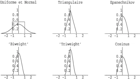
0.2.3.1. Exemptes de fonction noyau
Un des noyaux les plus utilisés est le noyau gaussien donné par K(t) = e_t2/2,
e
R.Dans les noyaux à supports compacts on peut citer le noyau “cosinus” donné par K(t) = cos (t) I(t < 1).
K(t) = c (1 —
ltD5
I(ltl
< 1), c.r, Eu voici quelques-mis (K1) Uniforme ou rectangulaire (K2) Triangulaire (K3) Epanechnikov (K4) “Biweight”ou “Quartic” (K5) “Tri’weight”Ces fonctions noyaux sont représentées clans la figure 0.2.
o
o J
o,t
49/.2
FIG. 0.2. Graphiques de quelques fonctions noyaux.
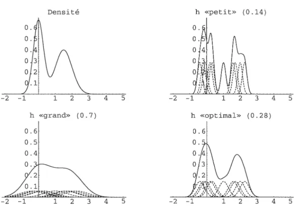
Example 0.2.1. On considère te mélange de deux normales suivant
Beaucoup de noyaux (à supports compacts) qui reviennent souvent dans la litté rature appartiennent à la famille suivante
r 2Bêta(s + 1, 1 s = 0, r s 1, r = 2, s = 1, r s = 2, r = 2, s 3,
Uniforme et Normal Triangulaire 1 0.8
j:
r>0,s>0. /r) cro = 1/2. e11 = 1. C21 = 3/4. C29 = 15/16. C23 35/32. Epanechnikov-f12
Cosinus 1 0.2Ï\2
—2—1 12 Triweight’ —2—1 12 ‘Biweiglit’ —2 12 —2—1N
12f:
0.5N(0, 0.09) + 0.5N(1.5,0.025)13 0. 0. o 0 0 Var (Jh(x)) = {(K * f)(x) - (Kh * f)2(x)}. f:O.5N(0,0.09) + 0.5N(1.5,O.025), n=10. Densité h «petit» (0.14) O. O 0 o h «grand» (0 .7) 0. 0. O. 0. .28)
FIG. 0.3. Différents résultats pour différentes valeurs de h.
et on dispose de n = 10 observations.
À
la figure 0.2., on trouve le graphiquede la vraie densité
f
ainsi que trois estimations correspondant à trois choix du paramètre h.0.2.3.2. Propriétés immédiates de Ï’estimateur à noyau
- L’estimateur
fi,
hérite, en général, des propriétés de la fonction K. Il sera, par exemple, continu, différentiable et une densité si K l’est. Aussi, il pourra prendre des valeurs négatives dans le cas où K en fait autant.- Biais
E (Jh(x)) = E (Kh(x - X)) = tKh * f)(x).
En pratique, c’est plutôt avec des expressions asymptotiques du biais et de la variance qu’on travaille. Pour cela, on a.joute des hypothèses sur
f
et K comme exiger def
cFêtre deux fois clifférentiable et les conditions suivantes sur KK>0,
f
K(u)du= 1,f
uK(n)du= 0,f
‘u2K(n)du <oo. Sous ces hypothèses de régularité on obtientBiais {fh(x)} = A(f, K) h2 + o(h2) (0.2.1)
Var{jh(x)} = B(f, K) + o
(),
(0.2.2) où A(f,K) ‘f”(x)fu2K(u)du et B(f K) Il en résulte que Biais {(x)} -+ 0, lorsque h 0.- Var {j(x)} 0, lorsqtie h O et nh oo.
- D’où MSE{fh@)}—*0, lorsque h—+0 et nh—*oo.
Aussi, la partie principale du développement du biais est croissante en h alors que celle de la variance est décroissante. Dans le choix du paramètre h, on devra faire un compromis entre le carré du biais et la variance.
0.2.3.3. Choix du rnéta-paramètre h
Les critères les plus utilisés pour le choix de h sont la MSE et la MISE, où MISE{!h}
=
f
MSE({!h(x)}dx.
Il s’agira alors de trouver le paramètre h qui minimisera l’une ou l’autre de ces quantités selon le choix. On distinguera ici les deux cas suivants
15
(a) Le cas où h est constant et on parlera alors de paramètre
global.
Pour l’obtenir, on minimisera la IVII$E. En fait, en pratique c’est plutôt une approximation de la MISE qu’on essayera de minimiser pour obtenir la quantité suivantehMIsE
= Ci(f,K), avec Citf,K)5
=
fu2Iu)duff»2tu)du
La valeur de h obtenue dépend donc de quantités inconnues.
t
b) Le cas où h = h(x) est variable. On parlera dans ce cas d’un paramètrelocat. On le déduit en minimisant une approximation de la i\/ISE. On
obtient l’expression suivante
hMsE =C2tf,K), avec 02c,K)5=
f
tx) f
K2(u)du 2n /
f”2(x) (f
u2K(u)du)En pratique, on remplacera
f
dans les expressions précédentes par la densité de la loi normale par exemple. D’autres méthodes sont aussi utilisées pour déter miner le paramètre optimal h. La plus utilisée en pratique est la méthode dite de validation croisée. Avec l’histogramme, l’estimateur à noyau est le plus répandu et le plus étudié.0.2.3.4. Méthode du noyau adaptatifou variable
Une modification de l’estimateur à noyau classique est faite en faisant varier le paramètre h. Deux telles versions ont reçu une attention particulière
• Fenêtre locale t”local bandwidth”); le cas h = htx).
Plusieurs techniques (“observation dépendantes”) ont été proposées pour choisir la fenêtre (locale). On peut citer ici les travaux de Fan et aï.
t
1996), Hazelton t1996, 1999) et Farmen et Marron (1999.) Cependant, à distance finie, les études de simulations dans ces études n’ont pas montré de résultats prometteurs même lorsque comparés à des estimateurs à fenêtre fixe comme celui de Sheather et Jones t1991) (voir Hazelton, 2003).• Fenêtre adaptative (“sample-poillt adaptive bandwidth”); h = c(X).
Lafonction c est choisie de sorte que AMISE(!) est petite. Abramson (1982)
propose de prendre h f(X)—’/2. Une seconde façon de faire est celle de restreindre c à une certaine classe de fonctions, ensuite optimiser relative ment à un certain critère (Sain et Scott, 1996.) Pour plus de détails, voir Hazelton (2003).
BIBLIOGRAPHIE
[11 Altman, N., Léger, C., (1995). ‘Bandwidth seiectwn for keTnet distribution function estimation”. J. Statist. Plann. Inference 46, 195-214.
[21 Azzalini, A., 1981. “A note on the estimat?on ofa distribution function and quantites by a kernet method.”Biometrika 68 (1), 326-328.
[31
Bowman, A., Hall, P., Prvan, T., 1998. ‘73andwidth setection for the smoothing of distribution functons.” Biornetrika 85 (4), 799-808.[41 Chu, 1.5., (1995). “Bootstrap smoothing parameter seÏection for distribution function estimation.” Math. Japon. 41 (1), 189-197.
[5] Cs.ki E. (1984). “Empiricat Distribution function.”, Handbook of Statistics (P. R. Krishnaiah and P. K. Sen, eds), vol. 4, 405-430.
[6] Devroye, L. and Lugosi, G. (2001). “Combinatoriat Methods in Density Estimation”, Springer-Verlag, New York, Inc.
[7] Dvoretzky, A. Kiefer, J. and Wolfowitz, A. J. (1956) “Asymptotic minimax character of the sampte distribution function and of the classicat muttinomiat estimator,” Ann. Math. Statist., 27, No. 3, 642669.
[8] Efron, B., Tibshirani, R.J., (1993). “An Introduction to the Bootstrap.” Chapman & Hall, London.
[9] falk, M., (1983). “Relative eficiency and deficiency of kernet type estimators of smooth distribution functions”. Statist. Neerlandica 37, 73-83.
[10] Fan, J., Hall, P., Martin, M. & Patil, p. (1996). “On local smoothing of nonpara metric curve estimators.” J. Amer. Statist. assoc. 91, 258-266.
[11] Farmen, M. et iViarron, J. (1999) “An assesment of finite sample performance of adaptive methods in density estimation.” Comput. Statist. Data Anal. 30, 143-168. [12] Finkelstein, H. (1971). “The Law of the Iterated Logarithm for empiricat distribu
[13] Hazelton, M. (1996). “Bandwidth selection for local density estirnators.” Scand. J. statist. 23. 221-232.
[14] Hazelton M. (1999). “An optimal local banclwidth selector for kernel density esti mation.” J. Statist. Plann. Inference 77, 37-50.
[151
Hazelton M. (2003). “Variable kernel density estimation.” Aust. N. Z. J. stat. 45(3), 271-284.[161 Jones, MC., 1990. “The performance of kernet density functions in kernet distribu tion function estimation.” Statist. Probab. Lett. 9, 129-132.
[17] Lehmann, E.L., Casella, G. (1998.) “ Theory of Point Estimation.” 2ncl ed., Sprin
ger, New York.
[18] IVlarnmitzsch, V., (1984). “On the asymptoticatÏy optimat solution within a certain ctass of kernet type estimators.” Statist. Decisions 2, 247-255.
[19] Massart, P. (1990). “The Tight Constant in the Dvoretsky-Kiefer-Wotfowitz Inequa tity”. Annals of probability, 1$: 1269-1283.
[20] Nadaraya, E.A., (1964). “Some new estimates for distribution functions”. Theory Probab. AppI. 15 , 497-500.
[21] Reiss, R.D., (1981). “Nonparametric estimation of smooth distribution functions”. Scand. J. Statist. 8, 116-119.
[22] Sain, S. et Scott, D. (1996).”On tocatty adaptive density estimation”, J.A.S.A., 91, 1525-1534.
[23] Sarda, p., (1993). “Smoothing parameter setection for smooth distribution func tions”. J. Statist. Plann. Inference 35, 65-75.
[24] Serfiing, J. Robert (1980). Approximation Theorems of Mathematicat Statistics”, John Wiley & Sons, Inc.
[25] $hao, Y., Xiang, X., (1997). “Some extensions of the asymptotics of a kernet esti mator of a distributiôn function.” Statist. Probab. Lett. 34, 301-308.
[26] Sheather, S., et Jones, M. (1991). “A retiabte data-based bandwidth setection method for kernet density estimation”, J.R.S.S., Series B 53, 683-690.
19
[271 Shirahata, S., Chu, 1$., (1992). “[ntegrated squared error of kernet-type estimator
of distributionfnnction’ Ann. Inst. $tatist. iVIath. 44 (3), 579-591.
[281 Stute, W. (1982). “The oscitatiori behavior of empirzcatprocesses.”Ann. Probability, 10, 86-107.
[291 Swanepoel, J.W.H., (1988). ‘Mean integrated squared error properties and optimat kerneis when estimating a distribution function”. Comm. Statist. Theory Methods 17 (11), 3785-3799.
[301 de Uii.a-Alvarez, J., Gonzâlez-IVlanteiga, W., Cadarso-Sudrez, C., (2000) “Kernet distribution function estimation under the Koziot-Green modet.” Journal of Statistical Planning and Inference 87, pp. 199-219.
[311 Watson, G. S., Leadbetter, M. R. (1964) “On the estimation of the probabitity density.” I. Ann. lVlath. Statist. 34 480—491.
[321 Winter, B. B. (1979) “Convergence rate of perturbed empiricat distribution func tions.” J. Appi. Probab. 16, no. 1, 163—173.
E$TIMATING THE CDF BY A
PERTURBATION 0F THE EDF
“Distributions are the numbers of the future.” Berthold $chweizer.
21
Abstract.
In this paper, we propose a new noilparametric approach for estimatrng a cumiila tive distribution function F using fuite mixtures. The properties of the proposed estimator are studied. We are able to obtain the same asymptotic statistical pro perties as those obtaineci using the empirical distribution function, under the
same minimum reguÏarity conditions. Uniform resuits for fixeci sample sizes are also obtained. Simulations ancÏ examples illustrate the approach.
Key Words : Non-parametric cclf estimation, Aclaptive smoothing, Spiines, Uni form consistency, Convergence in law.
1.1.
INTRODUCTIONWe are interested in estimating a cumulative distribution function (cdf) F with support on au intervalI of R, boundeci or not, baseci on a sample X1,. . . ,
from F. Several works have been devoteci to the estimation of a cdf. Most of these works require regularity conditions such as the existence of the density function, the clensity being Lipschitz or F being twice clifferentiable, for example. Our aim is to obtain a s7nooth estimation when necessary with strong asymptotic resuits
such as those obtainecl using the empirical distribution function under the same regularity conditions. Furthermore, we wish to obtain interesting results even for small sample sizes. We hope, on the basis of the theoretical ancl simulation results we obtain, that the reader will be convinced we achievecl these goals.
The most frequently used estimator for a cclf F is the empirical (sample) distribution function (ecÏf) F, where F(x) = I(X < x)/n (I being the
inclicator function). Here nF(x) has a binomial distribution B(n, F(r)) ancl F indicates the location of the observations. Also, the ecif has a long list of good statistical properties such as it is first order efficient in the minimax sense and F(x) is the unique minimum variance auJ unbiasecl estimator of F() (see Dvo retzky & al. (1956) ancl Lehmann & Cassella (1998), chapter 2). Furthermore, the edf is the llonparametric maximum likelihood estimator of F aiid plays a central role in nonparametric simulation ancl bootstrap (see Efron anci Tibshirani (1993), p. 310.) For a review of some properties of the edf see, e.g., Csâki E. (1984), Stute (1982) and Serfiing (1980). The fact that F is a step function even when the underlying cdf F is continuous, has called for the need (in certain areas of application like estimating the density) for smooth(er) estimators of F. Many smooth estimators have been proposed in the literature. lVIost of these estimators are based on smoothing the edf. One that has been extensively studied is the ker nel estimator, say Fh. Nadaraya (1964) established, under appropriate regularity conditions, the almost sure uniform convergence of Fh,. Watson and Leadbetter (1964) proved the asymptotic normality of Fh, Winter (1979) showed that F,. has
23
the Smirnov-Chung property. Azzalini (1981) deriveci an asymptotic expression for the mean squared error of F,,. Falk (1983), IVlammitzsch (1984), $wanepoel (1988) and Jones (1990) analyzecl mean integrated squared error properties of
F,,, proving that the smoothecl estimate is asymptotically more efficient than the empirical one. Shirahata and Chu (1992) showed that the superiority of kernel es timators is not necessarily true in the sense of the integrated squared error. Sarcla (1993), Altman ancl Leger (1995) and Chu (1995) are devoteci to the problem of bauclwidth selection for F,,. See as well $hao S Xiang (1997), Bowman ancl al. (1998) anci Alvarez anci al. (2000). Alternative methocis have been proposed as well.
Several estimators using spiines have been investigatecl. Wahba (1976) propo sed the methocl calleci histospiine (a spline-smoothecl histogram) which uses a dubic spiine to smooth the eclf. Restie (1999) propose another estimator based on smoothing the edf using cubic spiines. He and Shi (1998) use quadratic spiines to estimate the cdf. We may mention as weÏl Ramsay (1998, 1988) who uses mono tone (regression) spiines to estimate a monotone function.
Nonparametric Bayesian estimators have been proposeci by, e.g., Perron & Mengersen (2001) who use mixtures of triangular distributions (quadratic spiines). Hansen Lauritzen (2002) use Dirichiet processes to model the prior to estimate a concave cdf.
Chaubey and Sen (1996, 2002 (multivariate)) propose the estimation of a smooth cdf F, based on a Poisson operator (using Hille’s theorem) to smooth the edf. Babu and al. (2002) propose an estimator based on Bernstein topera tor) polynomials to smooth the edf. For other approaches ancl references see, e.g., Efromovitch (2001).
In order to estimate a cdf F, we start from the fact that the best estimation baseci on the observations cannot do better than the best approximation based on the fact that F is known. The present work has two goals. The first one is to develop a method for approximating a cdf F. The aim is to approximate the
space of ail cdf on the interval I by a finite dimensional space, of dimension m, say. The second one is to apply the approximation to the ectf F and therefore to estimate F. We woulcl like to mention here that our estimator is not necessarily smooth. In fact, our approach concerns the estimation of a cclf without further conditions on the ftmction F.
When F is known (section 2), a basic approximation G of F is a step function, with (cliscontinuity) jumps of the same amplitude. It is then enough to choose m jumps in the interval I in order to obtain an approximation G such that — GHœ < 1/2(m + 1) (uniform ripper bound). The problem then reduces to determining the location of the jumps (i.e., the nodes), this is an m-dimensional problem. Stili, one might prefer other options than working on step fiinctions. Therefore, we seek for smoother alternatives to the step function G. In section 2, we develop an approach, where by using a s’moothing parameter k, we are able to construct an approximation Gk, in the form of a finite mixture of cdfs (we call basis functions), such that, using m nodes, we obtain F — GkWœ < k/2(m + 1). furthermore, in our construction, we allow the possibility of using an instrumental function H which, when chosen close to F, helps in obtaining a better approxi mation (in fact, when H is taken as F, then G F, see lemma 2.3). By analogy to the Bayesian approach, the function H is seen here as a “prior” distribution (a pseudo prior.) The basis functions, that enter in the definition of G, possess a hierarchical structure, with supports that depend on a vector of nodes. Each cdf (descendent), element of the basis, is a mixture of two cdfs (generators) at a lower level, and the mixture of the two is performed using a third (fixed) cdf, say H. A choice of the nodes that ensures a uniform bound to F—GWœ is given in Lemma 2.2. A construction of the basis is given in section 2.3. The approximation G is smooth in general but it allows for discontinuity jumps when necessary/suitable. We think that the approximation resuits we obtain are new and could be used in approximation theory. In particular, we give a probabilistic interpreta tion to our construction which allows, among other things, to show in a simple
25
way how the construction of monotone spiilles gives the property of monotonicity. In particular, we construct the monotone spiine basis in a probabilistic mariner (which presents an interest in itself). Furthermore, we think that, the (parameter) function H and the role it plays in the approximation process, is unique to our method.
When F is unknown (section 3), we apply the approximation to the edf F. The ecif is then useci to choose tire nocies (among the orcier statistics) that clefine the supports of the basis functioris anci thus ciefine the estimator
Ê
of F (Lemma 3.1). With the right choice of the nocies, we obtainFnʜ
<k/2(m+1), which allows us to prove almost sure uniform convergence ofÊ
to F (Lemma 3.2). We then give, under certain conditions on in and n, the rates of the Lœ convergence and the L convergence for p> 1. We show as well that the estimatorÊ
has the Chung-Smirnov property. In section 3.5, we estabÏish the asymptotic behavior of the estimator in terms of the convergence in law of /F—Ê0.
In sections 3.4 and 3.5, equivalent statistics to the Kolmogorov-Smirnov and the Cramér-Von IViises statistics are introduceci (where F is replaceci by F) . We then obtain similar asymptotic resuits to those obtained using F. In section 3.6, we give some uniform ripper bounds to the variance, bias, MSE, and other quantities (lemma 3.9). Note that, no other conditions on F than the fact of being a cdf is supposed here compared to other methods where, usually, F is set to be differentiable and sometimes twice differentiable. Furthermore, our approach works on bounded and unbounded supports with no need for transformations and adjustments that may cause a lost of certain (asymptotic) properties of the estimator.
In section 4, we present numerical simulations to illustrate the performance of the proposed estimator. We think that a series of examples will help iii un
derstanding the choices to make coilcerning different parameters involved in the construction of the estimator. Generai guidelines are given relatively to the choice of these parameters. Comparison to recent works are doue throughout the paper.
f inally, we woulcl like to mention that “direct” applications are considereci in fu ture works. Among these, the estimation of a density function (in progress), the estimation of the survival function anci relateci functions, and some bootstrap applications (smoothed bootstrap) are considered.
1.2. APPROXIMATION 0F FUNCTIONS AND PROPERTIES
In this section we discuss the problem of approximating a cumulative dis tribution function (cdf) F defineci on an interval I C R, i.e., a non-decreasing, continuous from the right function with values on the interval [0, 1] such that F@)(1 — F(x)) = O for ail x I.
Let us denote byF(I) the space of ail cdfs on I, and let us define for F1, F2 E F(I) the (usual supremum) metric, d31(F1, F2) = supF1(x) — F2(x), which we de
xEa
note by Fi — F2,0. The space (F(I), U81) is a complete metric space.
In a statistical setup, we may have X1, X2,.. . ,X7, a sample from a common
distribution Po, where the parameter depends on different quantities including a parameter F, F E F. Under a frequentist approach, we may consider the maximum likelihood estimator of O, but this is well known to lead to overfitting problems with the space F being too large. In a Bayesian context, we may instead estabuish a prior on
e,
the space of O, but this may be complicated since the space is infinite dimensional. The technical difficulties of working on F itself thus impel us to consider alternative finite dimensional approximate spaces.1.2.1. Approximation and loss
Assume that Fm = {H: E 2 c Rm} is a space of dimension in approxi
mating F.
Two questions arise What is the loss associated with the use of Fm instead of F, and can we find an approximate space Fm for which this loss is small?
27
A measure of loss associateci with the approximation of .F by .Fm can be given by Slip inf d5(F,H).
FEF HEFrn
Hence, )(.F,.Fm) is aiways bounded from above by one.
The second question may now be phrased as follows. Given e > O, can we find an approximate space .}. such that .Fm) < E? Anci, if so, is there a simple
upper bound on m? In practice we woulcl prefer to have both m and e small!. In the next section, we introcluce an approximate space that will achieve the goals set in this section. This approximate space consists of finite mixtures of cclfs.
1.2.2. The mixture
Let a = inf{x: x
e
I} anci b sup{x:e
I}. The approximate space .Fm, wechoose to work with is based on m points a Yi < < y < b called nodes (knots) ancl a parameter k called the smoothing parameter. For convenience, we
set yj=a forj=—k+2,...,Oandy=bforj=rn+1,...,m+k—1
(multiple nocles of order at least (k—1) at the end points a and b). Any Gk E
is a finite mixture anci satisfies the following representation
m+k— m+1 j+k—2
Gk Gk,
(k — 1)(m + 1)
Z Z
Gk,t,
i=1 i=1 t=i
with weights
min(j,k—1,m+k—j)
Wk3
(k—1)(m+1) for j=1,2,...,m+k—1.
The weights Wkj are therefore positive and add up to 1.
Each function Gk, is a cdf on the interval ‘k,j = [Yj—k+1,
yj]
forj
= 1, 2,. ..,
m +k—1. The elements Gk, are callecl basis functions. A construction of Gk, is given in the next section. We further suppose that ni > k — 1 > O. The function Gk thus defined is therefore an element of .F(I) (hence a cdf by construction).
1.2.3. The basis
The basis elernents are such that Gk. Gk,+1 for
j
1, 2, . . . ,m + k — 2. For convenience, we set Gk,o 1 andGk,m+k
O.There is a hierarchicai structure in the construction of the basis baseci on a fixeci ccifH I. Let us ciefine on ‘k,j,
j
= 1, 2,. . . ,in + k — 1, the following functionsHk,3 Hk:1
if H -k+1) <H (y),
I(c > y) if H(y_k+1) = H(y).
Then the hierarchical structure is the following
Step 1 (initial step) : Gi,(e) = I(x yj) for ail c I and
j
1,.. . ,in (Dirac ccif).Step t + 1 G1+1, Ht1, G1,_1 + (1 — H1+1,) G1,. Cleariy Gk, Gk,+1 for aiÏk andj,
j
= 1,2,...,m+k—2.The fact that Gk, is a cdf on ‘k,j = [yj—k+1,y] cornes frorn the next iernma.
Lemma 1.2.1. We have the following resuits,
(a) Let F1, F2 be two cdfs on I, an interval oJ R, szich that F1 > F2, and let F3 be a cdf on R.
The function F(2) deftned by
F(2) =F3F1+(1-F3)F2 is then a cdf on I.
(b) The function F2A3 = F3 + (1 — F3)F2 = F2 + (1 — F2)F3 is a cdf on I (the extreme case F1 1.)
In particular, if F1 = F2 = 1, then F(2) = 1.
(e) The function F13 = F3F1 is a cdf on I (the extreme case F2 O.)
In particular, if F1 = F2 = O, then F(2) = O.
29
(a) Let X1 be a random variable (r.v.) with cdf F1.
Let U be a r.v. inciepenclent of X1 and uniformly ciistributeci on [0, 1]. Set X2=F’ [(1—U)sup{F1(): <X1}+UF1(X1)].
The cclf of X2 is then F2 anci we have P[X2 > X1] = 1.
Let X3 be a r.v. indepenclent of (X1, X2) and with ccif F3.
If we clenote by X2 the second order statistic based on X1, X2, and X3, then
P[X(2) <x] P[X(2) <xX3 <]P[X3 <] + P[X2 <xX3 > x]P[X3 > j Fi(x)F3() + F2()(1 — F3())
= F(2)(x) for ail r g I,
recail that X1 X2 with probability one.
Note that F2 <F(2) <F1 and X1 <X(2) <X2 with probability one. (b) The function F2A3 is the cdf of the r.v. min(X2, X3).
(e) The function F13 is the cclf of the r.v. max(Xi, X3). D Remarks
(1) Suppose we have multiple nocles of multiplicity t at y, e.g., vi Yj+1
= Yj+t—1 , then we obtain G1, = G1,+1 = = G,+t_i and
therefore, Gt,+t_i(e) = Gt_i,+t_2(x) =••• = Gi,j(x) if y = Yj+t—1.
(2) If a node y is of multiplicity t with t > k, then the function G will have
ajump at y.
If H is continuons, then the amplitude of the jump is giveil by (t — k + 1)+/(m + 1), where a+ = max(0, a).
(3) If H is chosen as the cdf of a uniform distribution on I (bounded), then the basis functions Gk, become piecewise polynomials of degree k — 1 and the function G, becomes a monotone spline. So, for k = 4, e.g., the
approximation is a cubic (monotone) spline. (4) The function H may depend on the nodes.
0.4 0.2 Y-iYo0 Y; Y2Y3 Y4 0.8 0.6 0.4 0.2 — G.,4 G2,4
Y5Y6’1 Y iYo0 Y; Y2 Y3 Y4 Y;=Y61
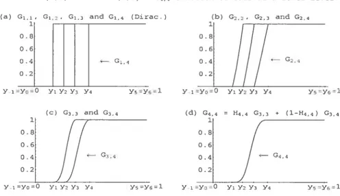
FIG. 1.1. The building of the basis function G4,4.
(5) If H is ftat between two iodes, then Gk is fiat between these two noctes. (6) If H has a cliscontinuity jump at a point x0, then Gk has a jlimp at x0. (7) In figure 1.1, we consider the case where F is the cclf of a Beta(2, 4), H is
taken as the cdf of a Beta(3, 3) anci we show the buildling of an element of the basis for k = 4, say G4,4 (cdf on [y,, y]) throw the clifferent stages
involveci. The function in (d) (G4,4) is the mixture of the two functions in
t
c)t
G3,3 and G3,4). Each function in tc) is a mixttire of two functions in (b), etc.1.2.4. The choice of the nodes and the parameters H and k
When k 1, Gj, is a step function. In order to obtain a good approximation for F, it is natural to set
y’=F’( m+1 where F’ is the generalized inverse of F,
1
(C) G3,3 and G3,4 (d) G4,4 = H4,4 G3,3 * (1—H4,4) G;,4
If
G34 04 [4YiYO0 Yi Y2 Y; Y4 Y1’Y6=l YiYo’0 Yi Y2 Y3 Y4 Y5Y61
31
For k > 1, we shah keep the same nodes. In fact, we have the following lemma
on the quality of the approximation.
Lemma 1.2.2. (Choice of the nodes)
If we take
y
F—’ (—T) for j = 1,.. . , m, then we obtairiF—Gk
Proof.
Let x I\{a, y,, . . . ,y, b}, then there exists j
e
{O, 1,.•• ,m} for which yj << We have, on the one hand ___
i+1
m+1 in+1
and on the other hand
i i+k—1
l—2(l)ZWkJ<Gk(X)<Wk3<l+2(l).
Hence for e
e
I\{a,yi, . . .,y,b}
k k
2(m+1) <F()—Gk(x)< 2(in+1)’ that is,
k
for ail xeI\{a,y,,...,y,b}. Finally, since F and G are continuous from the right, we obtain
FGkœ< D
It follows that for e> O given, we have )(F,Tm) <e whenever in> —1,
where .Fm is the approximate space of dimension in. We need to emphasize here
that the choice of the noches is reahly critical. The fllnction H is like a guess for F. When the nocÏes are adequately selected, a poor choice for H cannot be dramatic.
However, we hope that a perfect guess will imply that Gk = F for ail k > 1. In fact, this is t.rue in the case where F is continuous (see next lemma).
Lemma 1.2.3. (H F ,‘ Gj. F)
If F is a coritircuous cdf ou an interval I C R, y = F1(j/(m + 1)) for
j
=1,2,...,mandH=FthenGk=Fforaltk,k<m+1. Proof.
The proof is clone by induction on k, ru being fixeci. The resuit holcis for k = 2.
Suppose it is also true for k = 2,. . . , Ï, where t < ru + 1.
for ail x E R we have,
m+t Gi+1() = i= m+t = {Ht+;,(x) Gt,_1() + (1 — Hti,7(x)) Gi,(x)} j=1 = wt+y,jHt+j,y() Gto(x) m+t-1 +
{
wt+i,+iHi+i,+i(x) + wt+i,(l — Ht+1,(x))}
G(x) i=1 + Wt+1,m+t (1 — Ht+i,m+t()) Gt,m+i().Note that Gt,o(x) = 1 and Gt,m+t(.) = O, for ail x. Therefore,
Gt+i(x) = F(x)I(_œ,yy](X) + t(m+ 1) Ii,œ)(X) m+t-1 +
{
t wt,j Gi,(x) + F(x) — t( 1) I(+1](X) + t(m + 1) I(Yi+iœ)@)}.By induction, we have ‘T’1t’ w1, Gt,(x) = F(x) for ail x. Furthermore, we have
(1) I(_œ,yi](X) + I,1j(x) = 1.
m+t-1. m
(2) I(yi,œ)(X) — j=1 I — (j
33 (3) m+1—1 m
Z
I(yj+i,œ)(X) =ZI(ya+y,œ)(X)
i=1 i=1 In In m i1 =Z Z
‘y,y1j(x)Z Z
I(y,yy](X) j=1 i=j+1 i=2 j=1 In InZ
(i — 1) ‘(y,v+i1@) =Z
(j
— 1) I(yyj1](X) i=2 j=1Thus, Gt+1(x) = F(x) for ail x. D
Next, we give two examples. The first one concerns a smooth ccif, i.e., a
Beta(2, 4), anci the second one concerns a cdf with a discontiniity jump.
Example 1.2.1. Let F be the cdf of a Beta(2, 4) distribution. For illustration, we take k = 3, ru = 7 nodes only and for H we take a symmetric distribution on [0, 1], a Beta(3, 3) distribution. The function H is seen as a prior distribution. When no knowledge about F is available and I is bo’unded, we could choose H as the cdf of a uniform distribution for exampte. In figure 1.2., we have plotted the cdfs F and H (“the prior’) ami the corresponding densities
f
and h. Figure 2. e shows the plots of the approximation G together with F and the 9 functions ‘wkGk,. The weights a,t the end points are equal to 1/2(m + 1). In figure 2.d we have plotted the (absolute) error function F(x) — G(x) and we can see that— G,0 is retativety far from the uniform upper bound k/2(m + 1) = 1/4. Example 1.2.2. In this example, we consider a cdf F on [0, 1] with a disconti nuity jump at x = 1/2. The function F is given by,
t 1 z]’ x< F(x) = 1+ (2x— 1)2 otherwise. 2
There are multiple nodes at x = 1/2 so that G jumps at x = 1/2. For this
exampie we choose to take k = 3, ru = 10, 30, 50, and 100. The function H is
.2 0.4 0.6 0.8 1 of F, G and wGk,; 1 j 9.
/
G---/
/ Yo=O Y, YY,l[
Y 0I
Y2I
I
YI
116I
Y7 1Iii
Yj 0 0 0.1275 0.1937 0.2537 0.3138 0.3785 0.4541 0.5563 1 1 f(yj) 0 0 0.125 0.25 0.375 0.5 0.625 0.75 0.875 1 1 Gk(yj) 0 0 0.1023 0.2375 0.3652 0.4910 0.6158 0.7390 0.8530 1 1 Wk,j 1/16 1/8 1/8 1/8 1/8 1/8 1/8 1/8 1/16 FIG. 1.2. ExampleofaBeta(2,4).Gk, of the basis are piecewise potynomiats of degree 2 h— 1, SO that G becomes a quadratic (monotone) sptine. It is cl car that a prior k’nowtedge about this feature of F (the jump) wouÏd have made us choose another H that refiects this feature and therefore obtain a better approximation. This abitity of the approximation G, and thus of the estimator
Ê
(sec section 3), to be smooth in the regions where we expect F to be so, and to fotlow the jumps of F whenever there are, makes our method more generat than the competitors and helps us obtain better estimations for F. $ee figure 1.3. for graphies.(C) Plots 1 0.8 0.6 0.4 O 2 Flofs of P(x)-G(x) and k 2 (o.1) k 1 2 m fl 4 (4) 0.175 0.15 0.126 0.1 0.075 0.05 0.025 F-Gj 0.2 0.4 0.6 0.8 1
Plots of F and G for k=3, HoUnif(0,l) and m=l0,30,50,l00.
k=3 m=l0 k=3 m=30
0.2 0.4 0.6 0.8 1 0.2 0.4 0.6 0.8 1
k=3 m=50 k=3 m=100
0.2 0.4 06 0.8 1 0.2 0.4 0.6 0.8 1
FIG. 1.3. Example of a cdf on [0, 1] with a cliscontinuity jump at 1/2.
1.3.
EsTIMATIoN AND STATISTICAL RESULTSIn this section we apply the resuits of section 1.2 to the estimation of an unknown distribution function F F(I) basecl on a sample X1,.. . ,X0 from F.
Let F0(c) I(X < a)/n clenote the empirical distribution function and let us clenote G by
Ê
(where we drop the subscript k for simplicity). In the next subsections, we are going to look at the asymptotic behavior of the estimatorÊ
of F. In section 3.1, we give a uniform upper bounci to —Ê0.
In section 3.2 we establish the (almost sure) uniform convergence ofÊ
to F (lemma 3.2), then by aclding some conditions on m and n, we are able to give, in lemma 3.3, the rate of the uniform convergence. In section 3.3., we give a uniform upper bound to the L normÊ
—FU (p 1) (and by doing that we prove the L convergence ofÊ
to F and we give the rate of this convergence). In section 3.4, we define a Cramér-Von Mises like statistic and give a resuit relative to this one (lemma 3.6). In section 3.5., we define a statistic similar to the Kolmogorov-Smirnov one. We establish the convergence in law ofÊ
— F (lemma 3.9) and we show that the estimatorÊ
has the Chung-Smirnov property. We end the section by giving soine uniform results (uniform upper bounds) concerning the bias, variance, M$E,anci other quantities (lemma 3.11). We woulcl like to ilote here that by aclcÏing
some conditions on ni and n, we are able to obtain the asymptotic resuits ancÏ
properties that the Kolmogorov-Smirnov and the Cramér-Von Mises statistics have.
1.3.1. Distance of
Ê
to f,,When F is unknown, we use the ecif f,, to choose the nodes (among the order statistics). The selecteci nocles are given by yj = F’
(-)
forj
= 1,... ,m. In other words, we approximate the eclf. We have the next lemmaLemma 1.3.1. (Distance of
f’
to F,,)The above choice of the nodes implies that = and in this case we obtain
-
F2(m± 1)’
where
fal
= rnin{n Z: a < n} (the ceiling), and x denotes the orde’r statistics.In the case where rri n, me have y r loT 1
<j
<n and me obtain- F
2(n± Ï)•
We may compare tus upper bound to the one obtained in the paper by Babu and al. (2002) (theorem 2.2). In (4), the authors propose a (degree m polynomial) estimator Fn,m based on Bernstein polynomials and show that if F is differentiable with density
f
that is Lipschitz of order 1, tien at best we have— Fnœ
(Qon))3/4)
almost surely (when ra = n).
Compare this rate of convergence with the one in lemma 1.3.1. where we suppose F to be a cdf without further conditions.
37
1.3.2. Uniform convergence of 1 to F (Lœ convergence)
Using the previous lemma, we show that one cari obtain (almost sure) uniform convergence of
Ê
to F.Lemma 1.3.2. We have
lim
Ê
—
F = O a.s. (almost snrety).7n,n—*œ
P roof.
By taking y X(tn_._1) we obtain
-
FHœ < + UF-
F2(nr± 1) +
-Accordling to the Glivenko-Cantelli theorem,
—
File converges almost surely to O as n tends to oc. Therefore F—F converges almost surely to O a.s ra and n tend to oc .By acicling conditions on ra and n, we are able to control the rate of the uniform converge.
Lemma 1.3.3. (Rate of the uniform convergence)
If sup[n/(m2 loglog(n))] <oc, then
Ê
—F tends to O al’most s’arely at the rate loglog(n) Proof. We havef
Ê-F/
n <—
k/
nV
2 loglog(n)—
2(m + 1)V
2 loglog(n) + Fn_Filœj nV
2 loglog(n)And we have the resuit by noting that, by the law of the iterated logarithm, we have
—
File!
n <, with probabilityV
2 loglog(n) 21.3.3. L convergence of
Ê
to FLet us first recali the followillg inequalities
foreverys>land
x,y>O,
2’ (a + yS)< (x + y)S <S + y5, for every O < s < 1 anci
,
y
> 0,anci
P{FFnt}<2e_2flt2, forallt>0. For the la.st inequality, see iViassart (1990) anci Devroye (2001). We have the next lemma,
Lemma 1.3.4. Let p> 1 and Ïet us denote by the L-norrn, i.e.,
œ 1/p
f
G(x)dK@)) , for ail G,K We have < pF(p/2) + k -(2n)P/2 2(m+1)j
1 f[pF(p/2)]’/P k -i7 Proof. SinceÊ(x)
—F(x) < F — Fnœ + 2(m+ 1)’ for every x I, we obtainÊ(x)
- F(x) < -+ 2(m-+ 1)}
< 2’ {F — + [k ]P}39 it follows that, E-FF 2’ {E F-F+
[21T}
We obtaiii EUF —J
P(F — > t’/fl dt 2f
e2flt2 dt pJ
I2—1 e2 du - pf(p/2) — (2n)P/2 Hence, E-FW,F {-i [P(/) +[21ÏÏI”
i f[pr(p/2)]’/P k — 2’/ m+1 E 1.3.4. A Cramér-Von Mises like statisticThe Cramér-Von iViises statistic is given by (see, e.g., Serfiing (1980))
= n
f
[F) — F(x)]2 dF(). We have the following well known resuit,Lemma 1.3.5. (Finkelstein (1971)) With probabiÏity 1,
C1 1
lim
Let us clefine a similar statistic based on
Ê
in the following way= nJ [(x) - F(x)]2 dF(x),
so that we obtain the next lemma
Lemma 1.3.6. With probability 1,
k2 n 1
uni —lim + —.
2 loglog n 4 ni2 loglog
1.3.5. Asymptotic behavior of
f’
Let us recail the following welÏknown resuits (see Serfiing (1980), for example).
Theorem 1.3.1. (Kolmogorov, 1933)
If F is continuons and if we set DT, =
— fnœ, we obtain lim Pr(D <d) (_l)i e_232d2, U> 0.
3=—00
Theorem 1.3.2. (Smirnov, 1941)
Let us introduce the two quantities
sllp[F(x) — F(x)] and D sup[F() — If F is continuons, then we have the foltowing resuit,
1irnP(D>d)=1irnP(D>d)=e_2d2, d>0.
Lemma 1.3.7. (Asymptotic behavior of
Ê)
If F is continuons and ni is chosen such that > 0, then
n ,m—œ
lim Pr(b <U) = (—i) e_232d2, U> 0.
m,n—œ
j=-œ
41 Proof. We have - - - Fnœ < - F0w00 2(m± 1) Hence, 2(m±Ï) + \D0
<b,,
+ We obtain, Pr (Dn <d 2(m±1)) <Pr(br? <Pr (D <d+ 2(rn±1))’ ailci silice (Kolrnogorov’s theorem)lim Pr(D0 <d) = (—1) e_2j2d2, d> O,
n—oc
j=-œ
the resuit then follows. D
Lemma 1.3.8. Let us put,
= sup[](x) - f(x)] and
b
= sup[F(x) - F()]. If F zs continuons and rn is chosen such that - O, thenn m—oc
lirnP(b>d)=1imP(b>d)=e_2d2, d>O
Remarks
(1) The Chung-Smirnov property
Note that (cf. lemma 3.3.) ifm is chosen such that
TE
n/(m2 loglog(n)) =O, then
f
lias the Chung-Smirnov property, i.e.,TE
(2n/iog1ogn)’12 — Fil00 < 1, with probability(2) Pointwise convergence in law
If m is chosen siich that
TE
n/rn2 = O, then(fr(x)
- F(x))y
N (O, F(x)(1 - F(x)) for ail x.
(3) A Dvoretzky-Kiefer-Wolfowitz like inequality
Let us recali the two following inequalities
- F
2(m±1) + - F,
anci
P{UFFnWœ > t} for ail t >0.
Let {m}, Cm (0, 1), be a sequence of real nllmbers (close to 1), then we
obtain
P {UF — > t} <2e2t2,
whenever (m + 1)(1 — am) > k/(2t).
1.3.6. Some uniform resuits concerning the bias, variance, MSE, and other quantities
In the next lernima, we give uniform tipper bounds to the bias, variance, IVI$E,
and other quantities.
Lemma 1.3.9. We have the foltowing reszdts (a) Bias(F) = E (F — F)
2(+i) = 6m. Therefore F is asyrnptotically
unbiased. (b) MSE(1) <(6+1)2 <2(6+). (e) Var(Ê) (6m+)2 <2(6+). (d E
(w
- Hœ) 6m + (e) Var (MF - Êœ) <2 (6 + 1). Proof. (a) Bias, 6m.43
(b) MSE,
MSE(1) = E(1—F)2=E(î—F+F—F)2
F)2 + E(F - F)2}
(m+
2/ 2(m+).(e) Variance, Var
(])
< MSE (1). (cl) \Ve have, E (UF -E(Uf
- faœ) + E(M
-)
< + Srn. (e) We have Var (WF -= E (UF -)
- E2(UF -ÊWoe)
<E (HF -< E (F_Fnœ+Fn_F) < 2E (F_F+F_) < 2 (E F -+ <2 +1.4. GuIDELINEs ON THE CHOICE 0F THE PARAMETERS k, H, n-i
AND SIMuLATIoNs
We start t.his section by explailling the choïce of the clifferent parameters illvolvecÏ in the construction of the estimator, i.e., k, H, anci m. When rn and k
are chosen, we work with the nodes as in lemma 3.1. Here is a summary guiclelme to the choice of the parameters.
1. The choice of k (“the smoothing parameter “)
The parameter k is seen here as a smoothing parameter. The larger k,
the smoother the estimator. When H is taken as the cclf of a uniform distribution (on a boundeci support), the basis functions, Gk, become a
basis for the monotone spiines of order k — 1 (with variable nocles). So, to have a cubic spline, for example, we need to take k 4.
However, a large value of k renders the jumps of
f
more difficuÏt to obtain. In fact, to have a jump at y, a multiple node of orcler r (say y = Yj+1 == Yj+r—i), we neecl to have r> k.
In our simulations, we take k = 4, unless we have some knowleclge about
certain features of F.
2. Choice for H (the instrumental cdf)
By analogy to the Bayesian approach, H is seen as a prior distribution. In fact, if H is equal to F (not possible in practice), then we obtain excellent results as mentioneci in section 2 (lemma 2.3). A choice of H that is close to F will help mostly in the regions where F is fiat or almost fiat (in particular in the tails), that is, in those regions where the clensity
f
of F (when it exists) is very small. A prior knowledge about certain features of the distribution, like unimodality, asymmetry, concavity, discontinuity jumps, etc., dictates the choice of H, and therefore helps obtain a better estimation. When the support I of F is bounded but no other knowledge about F is available, H might be taken as the cdf of a uniform distribution.45
Note that when the support I of F is not bouncÏed, another choice than the uniform distribution is llecessary. This choice will have an influence on F in the tails. If H lias a cliscontinuity jump at a given point, the
estimator will present a jump at that same point. So a prior information of this kind help get a better estimation of F especially when the sample size is small.
3. The choice of ra (link between H and F)
The parameter ‘m = ra(n) clepencis on n in general. When H is smooth,
small values for ra induce a very smooth F. Whereas large values of ra make
Ê
stick to F, the ecif, but stiil remains smooth (unless we haveenough multiples iodes to make
Ê
jump).By analogy to Kernel methods, we may compare 1/ra to k, the banci wiclth (winclow). Recail (lemma 3.7) that by choosingrasuch that n/ra2 —*
O, we are able to obtain the asymptotic distribution of — FHœ. $0,
we might use this condition to help us choose ra.
The choice of ra is also associated with H. If one strongly believes that H is close to F, then choosing ra small is good. Furthermore, if ra is small relatively to n then the spacings will be very stable. Ifra is small,
f
lookslike H and if ra is large,
f
looks like F. Note that the choice of ra is more important than the choice of k.1.4.1. Numerical examples
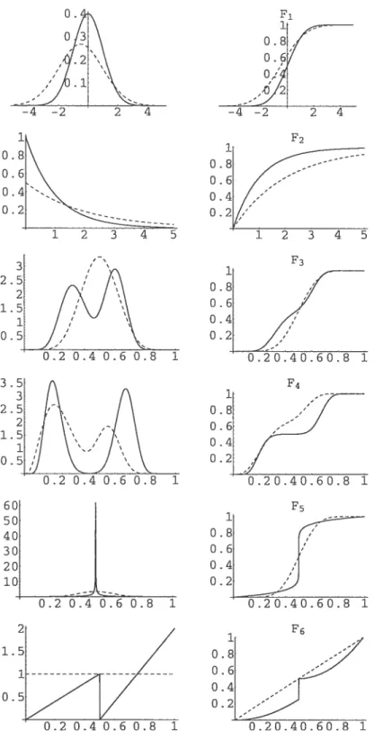
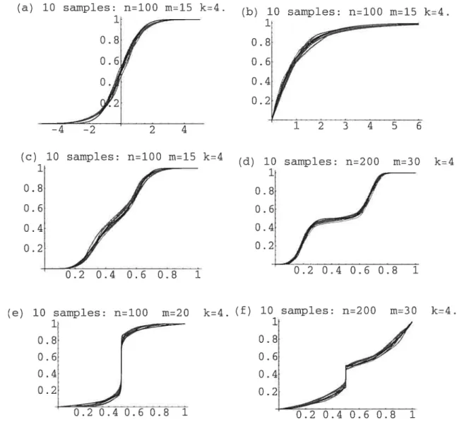
To illustrate the performance of the estimator, we have chosen six examples, four of which concern cdfs with bounded supports and two with unbouuded oies. Ii figure 1.4. we have plotted the cdfs aid corresponding densities of the selected distributions together with the chosen cdf H (dashed). For each of these cdfs, we have computed 10 estimates and plotted them together with the respective true distribution (cf figure 1.5) In what follows, we comment the results obtained for the corresponding examples (cf figure 1.5)
(a) The standard normal; N(O, 1)
In the case of the standard normal dlistribution, we choose to take H as a N(—0.5, (1.5)2). In figure 1.5 (a) we show the graphics of 10 estimates
from 10 samples with n = 100, m 15, ancl k = 4.
(b) The exponential distribution; Exp(1)
For the exponential distribution, we choose to take H as the cclf of an Expo(0.5) (“large variance.) In figure 1.5 (b). we show the graphics of 10 estimates from 10 samples with n = 100, ra = 15 anci k 4.
(c) Mixture of beta distributions
We choose to take the following mixture
Beta(10, 20) + Beta(30, 20).
The function H is taken symmetric to refiect “absence” of prior knowleclge, we choose to use a Beta(9,9).
We have taken 10 samples with n = 100, ra = 15, anci k = 4. We cari see
in figure 1.5 (c). that the estimator does quite well. For our simulations, we take k = 4 in general, unless we know about a particular feature in F,
like being very smooth. In this case, we may take k greater than 4.
(d) Another mixture of beta distributions (with a flat region) We choose to take another mixture with a fiat area, that’s
3eta(10, 40) + Beta(40, 20).
We choose for H the following mixture 2/3 Beta(4, 13) + 1/3 Beta(25, 20) (suppose we had a prior knowledge that F was bimodal and we had an idea where the modes were).
We have taken 10 samples with n = 200, ra = 30, and k = 4. We cari
47
knowledge ahollt the fiat region would have helped in obtainïng a better estimation.
(e) A cdf with an infinite derivative We take the following cdf on [0, 1],
1—(1—2c) 1
1f 3<—
F(r)=r 2 2
1+(2c—Ï) .
2 otheiwise
The ecif H is chosen as a Beta(10, 10) (symmetric). We have taken 10 samples with n = 100, m = 20, anci k = 4. It is clear that no polynomial
basecl estimator woulcl have followed the infinite slope. (f) A distribution with a jump
Like in example 1.2.2, we consicler a cdf F on [0, 1] with a cliscontinuity jump at x = 1/2. The hinction f is given by,
if x<—
=
i + — 1)2
2
2 otherwise.
The cdfH is chosen as a U(0, 1) to reftect the fact that no prior knowleclge is available. We have taken 10 samples with n 200, ru = 30, anci k = 4.
Figure 1.5 (f). shows that the estimator does well. An accumulation of nodes provokes the jump in
Ê.
Clearly, another choice of H reftecting the discoiitinuity jump would have lead to a better estimation.0.8 0.6 0.4 0.2 1 0.8 0.6 0.4 0.2 1 0.8 0.6 0.4 0.2 1 0.8 0.6 0.4 0.2 1 0.8 0.6 0.4 0.2 —2 2 4
FIG. 1.4. Plots of the distributiolls with the respective chosen H.
used for numerical evaluations
1 1 2 3 4 5 12 3 45
![FIG. 1.3. Example of a cdf on [0, 1] with a cliscontinuity jump at 1/2.](https://thumb-eu.123doks.com/thumbv2/123doknet/7753956.253804/46.918.232.763.110.397/fig-example-cdf-cliscontinuity-jump.webp)