HAL Id: hal-01225548
https://hal.archives-ouvertes.fr/hal-01225548
Submitted on 4 Dec 2015
HAL is a multi-disciplinary open access
archive for the deposit and dissemination of
sci-entific research documents, whether they are
pub-lished or not. The documents may come from
teaching and research institutions in France or
abroad, or from public or private research centers.
L’archive ouverte pluridisciplinaire HAL, est
destinée au dépôt et à la diffusion de documents
scientifiques de niveau recherche, publiés ou non,
émanant des établissements d’enseignement et de
recherche français ou étrangers, des laboratoires
publics ou privés.
ad hoc networks
Liang Zhou, Yan Zhang, Joel Rodrigues, Benoit Geller, Jingwu Cui, Baoyu
Zheng
To cite this version:
Liang Zhou, Yan Zhang, Joel Rodrigues, Benoit Geller, Jingwu Cui, et al..
Quality-delay
tradeoff for video streaming over mobile ad hoc networks.
ICC, 2012, Ottawa, Canada.
�10.1109/ICC.2012.6363798�. �hal-01225548�
Quality-Delay Tradeoff for Video Streaming over
Mobile Ad Hoc Networks
Liang Zhou
†, Yan Zhang
‡, Joel Rodrigues
♥, Benoit Geller
♦, Jingwu Cui
†, Baoyu Zheng
††
Key Lab of Broadband Wireless Communication and Sensor Network Technology (Nanjing University of Posts
and Telecommunications), Ministry of Education, China
‡
Simula Research Laboratory, Norway
♥
Instituto de Telecomunicac¸˝oes, University of Beira Interior, Portugal
♦Lab. of UEI, ENSTA-ParisTech, France
Abstract— In this work, we study the quality-delay tradeoff
for video streaming over mobile ad hoc network by utilizing a class of scheduling schemes. We show that node spatial mobility indeed impacts on the performance of wireless video transmission under the assumption that all the nodes can identically and uniformly visit the entire network. To describe a practical mobile scenario, we consider a random walk mobility model in which each node can randomly and independently choose its mobility direction at each time-slot. The contributions of this work are twofold: 1) It investigates the optimal node velocity for the mobile video network which helps to identify the impact of mobility on the video performance; 2) It derives the achievable quality-delay tradeoff range for any node mobility velocity, and thus it is helpful to design appropriate quality and delay requirements. These results provide insights on network design and fundamental guidelines on establishing an efficient mobile wireless video transmission system.
Index Terms— Wireless ad hoc network; video transmission;
quality; delay; tradeoff.
I. INTRODUCTION
I
N recent years, there has been a tremendous increase in demand for video communications over mobile ad hoc networks, and the corresponding techniques can fall into three categories [1]–[5]: 1) designing efficient media-aware routing, scheduling and resource allocation algorithms in the frame-work of cross-layer design; 2) developing novel source/channel coding algorithms aiming at adapting video frames to optimal bit-rate streams, such as multiple description coding, scalable video coding; 3) providing pervasive multimedia service envi-ronment by combining an adaptive service provisioning with a context-aware multimedia middleware.In contrast to the abundance of the above mentioned techniques, few literature focuses on how the mobility, e.g., the direction and velocity of the node mobility, impacts the performance of video streaming over wireless networks. Fig. 1 presents the results of a simulation study that compares the video quality (in terms of PSNR) with different node veloci-ties. Specifically, the simulation settings and video scheduling schemes are the same with that of [3]1. All the nodes follows
a random walk mobility model, i.e., they can randomly and independently choose the mobility direction at each time-slot
1Since this paper does not consider a multi-channel scenario, for fair
comparison, we set the channel number as 1 in [3].
0 5 10 15 20 25 30 34 36 38 40 42 P S N R ( d B ) Time (s) V=0 m/s V=1 m/s V=2 m/s V=3 m/s
Fig. 1. Video quality comparison for wireless ad hoc networks with different node velocities.
(the precise definition of this model is presented in Section II). From the given results, we can observe that: compared to PSNR value of the node immobility case (𝑉 = 0𝑚/𝑠),
𝑉 = 1𝑚/𝑠 gets almost the same performance, 𝑉 = 2𝑚/𝑠
is better in some extent, and 𝑉 = 3𝑚/𝑠 is consistently and dramatically better. This is an interesting phenomenon which motivates us to investigate the properties of wireless video transmission in the context of mobile environment, preferably in a quantitative manner.
The objective of this work is to make a pace towards clarifying how the node mobility impacts video streaming over wireless ad hoc networks. We bridge the theoretical analysis of fundamental disciplines of mobile video communications with the development of distributed wireless video scheduling. Under what conditions is it possible to achieve the optimal video quality given the transmission delay constraints for the mobile ad hoc networks? How efficiently can video streams be transmitted in the network? And to what extent does one can achieve the quality-delay tradeoff range? These questions are the main focus of this work.
The rest of this paper is organized as follows. In Section II, we present corresponding system models for video streaming over mobile ad hoc networks. In section III, we summarize our main results on the achievable quality-delay tradeoff range for
1 1 Source-1 Destination-1 2 1
Node One Hop Node Mobility
2 3 4 5 6 7
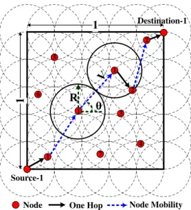
Fig. 2. Node random walk mobility model.
each velocity, and the rigorous proofs are given in Section IV. Finally, we conclude with a discussion of the contributions in Section V.
II. SYSTEMMODEL
A. Mobility Model
There are 𝒩 = {1, ..., 𝑛, ..., 𝑁} (𝑁 ∈ ℕ) nodes which are positioned in a unit torus square, i.e., the left and right edges are assumed to touch each other and the top and bottom edges are also connected to each other. Without loss of generality, each node is both a source and a destination, and all the nodes can identically and uniformly visit the entire network area. Each node’s transmission range is 𝑅 (𝑅 ∈ ℝ+), which is a constant parameter in this work. The video transmission delay is divided into some time-slots with unit length. In order to depict a practical mobile network scenario, we consider a general Random Walk Mobility Model (RWMM). Specifically, at the beginning of each time-slot, each node uniformly select a random mobility direction 𝜃 ∈ [0, 2𝜋). Then, the node moves along this direction with a constant velocity 𝑉 (𝑉 ∈ ℝ+) during the rest of time-slot. The mobility directions of the nodes can be selected again after each time-slot, totally independently from time-slot and node. Fig. 2 illustrates the behavior of RWMM.
B. Network Model
There are𝒵 = {1, ..., 𝑧, ..., 𝑍} video flows in the networks, for each flow 𝑧, it can be categorized into one of 𝐾 classes (i.e., 𝐶1, ..., 𝐶𝐾). In addition, a class𝐶𝑘 can be modeled as a triplet (𝐷𝑘, 𝑊𝑘, 𝜆𝑘): 𝐷𝑘 represents the delay deadline of
𝐶𝑘; 𝑊𝑘 is the average source rate of each flow in 𝐶𝑘; 𝜆𝑘
denotes the quality impact factor of𝐶𝑘. We refer the interested readers to [4] for more details on how these parameters can be extracted.
Let ℰ be the available link set in the wireless networks, and each link 𝑙 ∈ ℰ is a memoryless packet erasure channel.
IEEE 802.11a standard is deployed to access the channel. We denote the packet loss rate over link𝑙 for a flow in class 𝐶𝑘as
𝑝𝑙,𝑘, which can be approximated using the sigmoid function
[4]. Moreover, we denote 𝑇𝑙,𝑘 to represent the maximum transmission rate for class𝐶𝑘streaming over link𝑙. According to [3], the effective transmission rate for flow 𝑧 transmitting over link 𝑙 can be computed by 𝑇𝑙,𝑘(1 − 𝑝𝑙,𝑘)𝑡𝑙,𝑧, where 𝑡𝑙,𝑧 shows the time sharing fraction for video flow 𝑧 streaming over link𝑙. In particular, 𝑡𝑙,𝑧= 0 shows that flow 𝑧 does not stream over link𝑙.
C. Video Scheduling
We define the scheduling of a video flow𝑧 as 𝑥𝑧= {𝑡𝑙,𝑧}, and let 𝒳 = [𝑥1, 𝑥2, ...𝑥𝑍] be the joint scheduling for all 𝒵 video flows.𝐷𝑧(𝒳 ) represents the delay for transmitting the flow 𝑧 from source to destination based on 𝒳 . According to previous models,𝐷𝑧(𝒳 ) can be given by [4]:
𝐷𝑧(𝒳 ) =
∑
𝑙,𝑡𝑙,𝑧>0
𝐿𝑘
𝑡𝑙,𝑧(1 − 𝑝𝑙,𝑘)𝑇𝑙,𝑘, 𝑧 ∈ 𝐶𝑘, (1)
where 𝐿𝑘 is the average packet size of 𝐶𝑘. Therefore, the received video quality from node 𝑛, denoted by 𝑄𝑛, can be expressed as: 𝑄𝑛(𝒳 ) = 𝐾 ∑ 𝑘=1 𝑁𝑛𝑘 ∑ 𝑧=1 𝜆𝑘⋅ 𝑊𝑘⋅ 𝐼(𝐷𝑧(𝒳 ) ≤ 𝐷𝑘), (2)
where 𝑁𝑛𝑘 is the number of flows in class 𝐶𝑘 from 𝑛 and
𝐼(⋅) is the indicator function [4]. Therefore, the wireless video
scheduling can be formulated as arg max 𝒳 {∑𝑁 𝑛=1 𝑄𝑛(𝒳 ) } , (3) 𝑠.𝑡. ∑𝑍 𝑧=1 𝑡𝑙,𝑧≤ 1, ∀𝑙 ∈ ℰ, (3.1) 𝐷𝑧(𝒳 ) ≤ 𝐷𝑘, ∀ 𝑧 ∈ 𝐶𝑘, 𝑧 = 1, ..., 𝑍, 𝑘 = 1, ..., 𝐾. (3.2)
Specifically, (3.1) is the resource constraint for each link, and (3.2) is the delay constraint for each flow. In this paper, we employ the Distributed Minimum-Distortion Scheduling (DMDS) introduced in [3] as our operation rule2. It can be viewed as a member of the distortion-aware scheduling family. In short, DMDS studies the tradeoff between video quality and transmission delay the two competing objectives in a convex optimization formulation, and discusses the distributed solution by jointly utilizing multi-path routing and cross-layer design.
III. MAINRESULTS
Recall that we aim at studying the impact of velocity𝑉 on the average video quality 𝑄 and on the average transmission delay 𝐷 in the context of wireless ad hoc networks with RWMM. In particular, we define the∑ 𝑄 and 𝐷 as: 𝑄 ≜
𝑁 𝑛=1𝑄𝑛 𝑁 and𝐷 ≜ ∑𝑍 𝑧=1𝐷𝑧 𝑍 .
2We do not consider a wireless network with multiple channels, therefore,
Average Delay (D) A v er a g e Q u a li ty ( Q ) 1 N 1 N 1 Vt 4 1 Q D log N V N § · 4¨© ¸¹ 1 N Q D N 2 log N V N §§ ·· d 4¨¨¨© ¸¹¸¸ © ¹ log N V N § · 4¨ ¸ © ¹ 3N2 3 2 1/ N 3 N 1/ N 3 1/ N
Fig. 3. Quality-Delay scaling tradeoff (in log-log scale) for different velocities.
A graphical representation of our results is presented in Fig. 3. From the displayed result, we can observe that a wide range of quality-delay tradeoff is possible for𝑉 < Θ(1) in the framework of DMDS. For a given𝑉 , the feasible combinations of𝑄 and 𝐷 situate on a line departing from the common point
𝐷 = 𝑁, 𝑄 = 1 (which represents the maximum delay and
the best quality). The little circles, which situate on the line
𝑄 = 1/√𝐷, denote the smallest achievable delay for each 𝑉 (corresponding to the worst quality). We can also observe
that, when 0 ≤ 𝑉 ≤ Θ ((
log 2𝑁 2𝑁
)2)
, all points situate on the line 𝑄 = 𝐷𝑁. For 𝑉 ≥ Θ(1) no quality-delay tradeoff is achievable since the quality is maximized in conjunction with the minimization of delay.
IV. THEORETICALANALYSIS FORQUALITY ANDDELAY
Theorem 1: Let 𝑁 be the number of nodes in wireless ad
hoc networks, and 𝑉 be the each node’s mobility velocity. Using DMDS with the RWMM assumption, a wide range of quality-delay tradeoff is possible for any 0 ≤ 𝑉 < Θ (1) (shown in Fig. 3), in particular, the minimal values of𝑄 and
𝐷 satisfy 𝑄 = 1/√𝐷.
The proof of this theorem proceeds as follows. First we study the communication probability (Lemma 1) and hop numbers (Lemma 2) for any two nodes. Then, Lemma 3 and
Lemma 4 give lower bounds on the quality and delay
expec-tation value for each velocity, which implies (Corollary 1) that there is a relationship between each bound of quality and delay. We also show (Lemma 5) that there exists an achievable quality-delay tradeoff range for each velocity and this range is a linear function (Corollary 2).
We start by analyzing the probability of two nodes can communicate with each other. Let the probability of each node can communicate with any other nodes isℙ𝑐(𝑁, 𝑉, 𝑅), where
𝑅 is the each node’s transmission range, then we have the
following lemma.
Lemma 1: If𝜉 =
∑𝐾 𝑘=1𝑝𝑙,𝑘
𝐾√𝑉 +𝑅 log 𝑁, the value of ℙ𝑐(𝑁, 𝑉, 𝑅)
satisfies:
ℙ𝑐(𝑁, 𝑉, 𝑅) ≥ 𝑒−𝜉. (4)
Proof: Since this proof is similar to that of [6, Theo-rem 14], we omit it here.
Lemma 2: Assume that𝑁 and 𝑅 are known, for any 𝑉 ≥ 0,
let 𝜔1(𝑉 ) = ⌈ 𝜔2(𝑉 ) ℙ𝑐(𝑁, 𝑉, 𝑅) ⌉ , (5) 𝜔2(𝑉 ) = log 𝑁𝐾√𝑉 +𝑅 / 𝐾 ∑ 𝑘=1 𝜆𝑘𝑊𝑘 𝐷𝑘 , (6)
then under the DMDS with RWMM, the transmission delay from source to destination is finite, and the average number of the hops is not larger than∣𝜔1(𝑉 )∣.
Outline of the proof: We first introduce a theorem introduced
in [7]: Let {ℎ𝑚,𝑛} be a set of random variables satisfying 0 ≤ 𝑚 < 𝑛. Suppose that {ℎ𝑚,𝑛} has the following five
properties:
1) ℎ0,𝑛≤ ℎ0,𝑚+ ℎ𝑚,𝑛;
2) for each𝑛, 𝔼 (∣ℎ0,𝑛∣) < ∞ and 𝔼 (ℎ0,𝑛) ≥ 𝑐𝑛 for some constant𝑐 > −∞;
3) the distribution of {ℎ𝑚,𝑚+𝑘: 𝑘 ≥ 1} does not depend on𝑚;
4) for each 𝑘 ≥ 1, {ℎ𝑛𝑘,𝑛𝑘+𝑘: 𝑛 ≥ 0} is a stationary sequence;
5) The stationary sequence in 4) is ergodic. We can get: i) 𝜌 = limΔ
𝑛→∞ 𝔼[ℎ0,𝑛] 𝑛 = inf𝑛≥1𝔼[ℎ𝑛0,𝑛]; ii) 𝐻 =Δ lim 𝑛→∞ ℎ0,𝑛
𝑛 exists; iii)𝔼 [𝐻] = 𝜌; iv) 𝐻 = 𝜌.
Then, in order to apply the previous theorem to our problem, we make the following notations. Letℎ𝑚,𝑛 and𝐻𝑚,𝑛 be the multi-hop (maybe single-hop) delay and the number of hops from node𝑚 to node 𝑛, respectively. By the characteristics of DMDS and RWMM, it is obvious that conditions 1), 3) and 4) hold for{ℎ𝑚,𝑛}. We only need to show condition 2) and 5) also hold for {ℎ𝑚,𝑛}. The following procedure is same with in [7, Theorem 2].
Lemma 3: Assume that𝑁 and 𝑅 are known, let 𝑄 denote
the video quality and0 ≤ 𝑉 < Θ (1). Using DMDS with the RWMM, the expectation value of𝑄 is related to 𝑉 , and there exists a constant𝐵𝑄 (𝐵𝑄∈ ℝ+) enabling
𝔼[𝑄(𝑉 )]≥ 𝐵𝑄, ∀ 𝑉 ∈[0, Θ (1)). (7)
Similar to [6], we define a potential function Φ (𝑞) = ∑𝑁
𝑛=1(𝑄𝑛− 𝑄) and a variance function 𝑣𝑛(𝑞) =𝑁1 ∑
𝑛′∕=𝑛(𝑄𝑛− 𝑄𝑛
′). In order to prove Lemma 3, we
should use the following propositions.
Proposition 1: ∀ 𝑉′, 𝑉 ∈[0, Θ (1)), ∑𝑁 𝑛=1(𝔼[𝑄𝑛(𝑉′)] ∣𝑄 (𝑉 ) = 𝑞 )2= 𝑁𝑄2+ 𝑁 ∑ 𝑛=1𝑣𝑛(𝑞) 2. Proof: 𝑁 ∑ 𝑛=1(𝔼 [𝑄𝑛(𝑉 ′)] ∣𝑄 (𝑉 ) = 𝑞 )2= ∑𝑁 𝑛=1(𝑄 + 𝑣𝑛(𝑞)) 2 = 𝑁𝑄2+ 2𝑄 ∑𝑁 𝑛=1𝑣𝑛(𝑞) + 𝑁 ∑ 𝑛=1𝑣𝑛(𝑞) 2,
where the second term is zero due to the definition of variance function.
Proposition 2: ∀ 𝑉′, 𝑉 ∈[0, Θ (1)), there exists a constant
𝐵𝑄 (𝐵𝑄∈ ℝ+),
𝔼 [Φ (𝑄 (𝑉′)) ∣𝑄 (𝑉 ) = 𝑞 ] ≥ 𝐵
Proof: 𝐿𝐻𝑆 𝑜𝑓 (8) = ∑𝑁 𝑛=1 𝔼[𝑄𝑛(𝑉′)2∣𝑄 (𝑉 ) = 𝑞 ] − 𝑁𝑄2 = 𝑁 ∑ 𝑛=1 (𝔼 [𝑄𝑛(𝑉′) ∣𝑄 (𝑉 ) = 𝑞 ])2 + 𝑁 ∑ 𝑛=1 var (𝑄𝑛(𝑉′) ∣𝑄 (𝑉 ) = 𝑞 ).
Using the Observation 3.3 of [8], we can get the result.
Proof of Lemma 3: From Propositions 1, 2, we can get the
result of Lemma 3.
Lemma 4: Assume that𝑁 and 𝑅 are known, let 𝐷 denote
the transmission delay which is defined in Section II and 0 ≤
𝑉 < Θ (1). Using DMDS with RWMM, the expectation value
of 𝐷 is related to 𝑉 , and there exists a constant 𝐵𝐷 (𝐵𝐷 ∈ ℝ+) enabling
𝔼[𝐷(𝑉 )]≥ 𝐵𝐷, ∀ 𝑉 ∈[0, Θ (1)). (9) Proof: Since the proof process is similar to that of
Lemma 3, we do not repeat it here.
Corollary 1: Assume that 𝑁 and 𝑅 are known, for 0 ≤ 𝑉 < Θ (1), using DMDS with RWMM, all the lower bounds
of 𝑄 and 𝐷 lie on one curve.
Lemma 5: Assume that𝑁 and 𝑅 are known, let 𝑄 and 𝐷
denote the video quality and transmission delay. Using DMDS with RWMM, a wide range of 𝑄 − 𝐷 tradeoff is possible for any 0 ≤ 𝑉 < Θ (1),
Proof: See Appendix.
Then we have the following corollary to describe the𝑄−𝐷 tradeoff range.
Corollary 2: For a given 𝑉 ∈ [0, Θ (1)), the feasible combinations of 𝑄 and 𝐷 lie on a line departing from the common point 𝐷 = 𝑁, 𝑄 = 1.
Now we can give the proof of Theorem 1.
Proof of Theorem 1: For a fixed 𝜂 > 0, when 0 ≤ 𝑉 <
Θ(1), we have: ℙ (𝑄 > 𝑞) = ℙ (𝑄 > 𝑞; 𝑁 ≤ 𝑞 (1 − 𝜂)) (10) + ℙ (𝑄 > 𝑞; 𝑁 > 𝑞 (1 − 𝜂)) < ℙ ⎛ ⎝⌊𝑞(1−𝜂)⌋∑ 𝑛=1 𝑄𝑛> 𝑞 ⎞ ⎠ + ℙ (𝑁 > 𝑞 (1 − 𝜂)) . Also, we can have a lower bound:
ℙ (𝑄 > 𝑞) = ℙ (𝑄 > 𝑞; 𝑁 > 𝑞 (1 + 𝜂)) = ℙ (𝑁 > 𝑞 (1 + 𝜂)) − ℙ (𝑄 ≤ 𝑞; 𝑁 > 𝑞 (1 + 𝜂)) ≥ ℙ (𝑁 > 𝑞 (1 + 𝜂)) − ℙ ⎛ ⎝⌊𝑞(1+𝜂)⌋∑ 𝑛=1 𝑄𝑛≤ 𝑞 ⎞ ⎠ . Specifically, using the Chernoff bound, we can show that there exists constants𝜅, 𝜄 such that
ℙ ⎛ ⎝⌊𝑞(1−𝜂)⌋∑ 𝑛=1 𝑄𝑛> 𝑞 ⎞ ⎠ < 𝜅𝑒−𝑞𝜄.
Thus, as𝑞 → ∞, it follows that
ℙ ⎛ ⎝⌊𝑞(1−𝜂)⌋∑ 𝑛=1 𝑄𝑛> 𝑞 ⎞ ⎠ = 𝑜 (ℙ (𝑁 > 𝑞)) , (11) ℙ ⎛ ⎝⌊𝑞(1−𝜂)⌋∑ 𝑛=1 𝑄𝑛≤ 𝑞 ⎞ ⎠ = 𝑜 (ℙ (𝑁 > 𝑞)) . (12) Go back to (10), we get lim sup 𝑞→∞ ℙ (𝑄 > 𝑞) ℙ (𝑁 > 𝑞) ≤ lim sup𝑞→∞ ℙ ( ⌊𝑞(1−𝜂)⌋∑ 𝑛=1 𝑄𝑛 > 𝑞 ) ℙ (𝑁 > 𝑞) + lim sup 𝑞→∞ ℙ (𝑁 > 𝑞 (1 − 𝜂)) ℙ (𝑁 > 𝑞) . (13) According to (11), the first term of (13) is zero, so that for all
𝜂, we have lim sup 𝑞→∞ ℙ (𝑄 > 𝑞) ℙ (𝑁 > 𝑞) ≤ lim sup𝑞→∞ ℙ (𝑁 > 𝑞 (1 − 𝜂)) ℙ (𝑁 > 𝑞) . (14) Taking the limit𝜂 ↓ 0, we can get
lim sup
𝑞→∞
ℙ (𝑄 > 𝑞)
ℙ (𝑁 > 𝑞) ≤ lim𝜂↓0lim sup𝑞→∞
ℙ (𝑁 > 𝑞 (1 − 𝜂)) ℙ (𝑁 > 𝑞) = 1.
(15) Similarly, we can also get:
lim sup
𝑞→∞
ℙ (𝑄 > 𝑞)
ℙ (𝑁 > 𝑞) ≥ 1. (16) (15) and (16) imply the results.
V. CONCLUSIONS
In this paper, we study the impact of mobility on video streaming over wireless ad hoc networks from the perspec-tives of video quality and transmission delay. In particular, our contributions are twofold. First, we have investigated the optimal node velocity for for the mobile video network under the random walk mobility model. This strategy helps to identify the contribution of mobility in the improvement the performance of video communications. Second, we present the achievable quality-delay tradeoff range for any node velocity. This point is very helpful for the network operators to de-sign an appropriate quality or delay requirement for general wireless video transmission.
ACKNOWLEDGEMENTS
This work is supported by A Project Funded by the Priority Academic Program Development of Jiangsu Higher Education Institutions–Information and Communication Engineering.
APPENDIX: PROOF OFLEMMA5
We first get an upper bound for the tradeoff when0 ≤ 𝑉 < Θ (1). For every 𝜂 > 0, we have
ℙ(∣𝜔1∣ ≥ 𝑞𝐵𝑄/𝐵𝐷; 𝑄 ≥ 𝑞)= ℙ(∣𝜔1∣ ≥ 𝑞𝐵𝑄/𝐵𝐷; 𝑄 ≥ 𝑞; 𝑄𝑛≤ 𝑞 (1 − 𝜂))+ ℙ(∣𝜔1∣ ≥ 𝑞𝐵𝑄/𝐵𝐷; 𝑄 ≥ 𝑞; 𝑄𝑛> 𝑞 (1 − 𝜂)) (𝑎) ≤ ℙ (𝑄 ≥ 𝑞; 𝑄𝑛≤ 𝑞 (1 − 𝜂)) + ℙ(∣𝜔1∣ ≥ 𝑞𝐵𝑄/𝐵𝐷+ 𝑞 (1 − 𝜂)) (𝑏) < ℙ ( ⌊𝑞(1−𝜂)⌋∑ 𝑛=1 𝑄𝑛> 𝑞 ) + ℙ(∣𝜔1∣ ≥ 𝑞𝐵𝑄/𝐵𝐷+ 𝑞 (1 − 𝜂)). (A1)
In (𝑎), we use Lemma 3, and in (𝑏), we useLemma 4. Next, we can derive a lower bound:
ℙ(∣𝜔1∣ ≥ 𝑞𝐵𝑄/𝐵𝐷; 𝑄 ≥ 𝑞)≥ ℙ(∣𝜔1∣ ≥ 𝑞𝐵𝑄/𝐵𝐷; 𝑄 ≥ 𝑞; 𝑄𝑛 > 𝑞 (1 + 𝜂))= ℙ(∣𝜔1∣ ≥ 𝑞𝐵𝑄/𝐵𝐷; 𝑄𝑛> 𝑞 (1 + 𝜂))− ℙ(∣𝜔1∣ ≥ 𝑞𝐵𝑄/𝐵𝐷; 𝑄 < 𝑞; 𝑄𝑛 > 𝑞 (1 + 𝜂))≥ ℙ(∣𝜔1∣ ≥ 𝑞𝐵𝑄/𝐵𝐷 + 𝑞 (1 + 𝜂))− ℙ ( ⌊𝑞(1+𝜂)⌋∑ 𝑛=1 𝑄𝑛≤ 𝑞 ) . (A2)
We can observe that the termsℙ ( ⌊𝑞(1−𝜂)⌋∑ 𝑛=1 𝑄𝑛 > 𝑞 ) in (A1) andℙ ( ⌊𝑞(1+𝜂)⌋∑ 𝑛=1 𝑄𝑛 ≤ 𝑞 )
in (A2) decay exponentially fast as
𝑞 → ∞ for any 𝜂 > 0. This is because each link calculates
the rates to achieve a balance between the rate increment and network congestion, and each source determines the optimal path distribution to achieve minimum video distortion in the framework DMDS. More precisely, a Chernoff bound can be used to get ℙ ⎛ ⎝⌊𝑞(1−𝜂)⌋∑ 𝑛=1 𝑄𝑛 > 𝑞 ⎞ ⎠ = 𝑜(ℙ(∣𝜔1∣ ≥ 𝑞𝐵𝑄/𝐵𝐷 + 𝑞 )) , (A3) and ℙ ⎛ ⎝⌊𝑞(1−𝜂)⌋∑ 𝑛=1 𝑄𝑛 ≤ 𝑞 ⎞ ⎠ = 𝑜(ℙ(∣𝜔1∣ ≥ 𝑞𝐵𝑄/𝐵𝐷 + 𝑞 )) . (A4) Case I: 𝐵𝑄/𝐵𝐷< 1. Using (A1), we have
lim sup 𝑞→∞ ℙ(∣𝜔1∣≥𝑞𝐵𝑄/𝐵𝐷;𝑄≥𝑞) ℙ(∣𝜔1∣≥𝑞) ≤ lim sup 𝑞→∞ ℙ (⌊𝑞(1−𝜂)⌋ ∑ 𝑛=1 𝑄𝑛>𝑞 ) ℙ(∣𝜔1∣≥𝑞) + lim sup 𝑞→∞ ℙ(∣𝜔1∣≥𝑞𝐵𝑄/𝐵𝐷+𝑞(1−𝜂)) ℙ(∣𝜔1∣≥𝑞) .
Since 𝐵𝑄/𝐵𝐷< 1, ∀ 𝜂 > 0 we can get lim sup 𝑞→∞ ℙ(∣𝜔1∣ ≥ 𝑞𝐵𝑄/𝐵𝐷; 𝑄 ≥ 𝑞) ℙ (∣𝜔1∣ ≥ 𝑞) ≤ lim sup𝑞→∞ ℙ (∣𝜔1∣ ≥ 𝑞 (1 − 𝜂)) ℙ (∣𝜔1∣ ≥ 𝑞) . Thus, lim sup 𝑞→∞ ℙ(∣𝜔1∣≥𝑞𝐵𝑄/𝐵𝐷;𝑄≥𝑞) ℙ(∣𝜔1∣≥𝑞) ≤ lim 𝜂↓0lim sup𝑞→∞ ℙ(∣𝜔1∣≥𝑞(1−𝜂)) ℙ(∣𝜔1∣≥𝑞) (𝑐) = 1, (A5) where(𝑐) comes from Lemma 2. Similarly, we can use (A2) and (A4) to get
lim sup 𝑞→∞ ℙ(∣𝜔1∣≥𝑞𝐵𝑄/𝐵𝐷;𝑄≥𝑞) ℙ(∣𝜔1∣≥𝑞) ≥ lim 𝜂↓0lim sup𝑞→∞ ℙ(∣𝜔1∣≥𝑞(1+2𝜂)) ℙ(∣𝜔1∣≥𝑞) = 1. (A6)
In fact, (A5) and (A6) imply that ℙ(∣𝜔1∣ ≥ 𝑞𝐵𝑄/𝐵𝐷; 𝑄 ≥ 𝑞
)
∼ ℙ (∣𝜔1∣ ≥ 𝑞) . (A7) Case II: 𝐵𝑄/𝐵𝐷= 1. We can easily get (A7).
Case III: 𝐵𝑄/𝐵𝐷 > 1. For the upper bound, from (A1) we can have lim sup 𝑞→∞ ℙ(∣𝜔1∣≥𝑞𝐵𝑄/𝐵𝐷;𝑄≥𝑞) ℙ(∣𝜔1∣≥𝑞𝐵𝑄/𝐵𝐷) ≤ lim sup 𝑞→∞ ℙ(∣𝜔1∣≥𝑞𝐵𝑄/𝐵𝐷+𝑞(1−𝜂)) ℙ(∣𝜔1∣≥𝑞𝐵𝑄/𝐵𝐷) ≤ 1. (A8)
Similarly, for the lower bound, from (A2), we can get lim sup 𝑞→∞ ℙ(∣𝜔1∣≥𝑞𝐵𝑄/𝐵𝐷;𝑄≥𝑞) ℙ(∣𝜔1∣≥𝑞𝐵𝑄/𝐵𝐷) ≥ lim sup 𝑞→∞ ℙ(∣𝜔1∣≥𝑞𝐵𝑄/𝐵𝐷+𝑞(1+𝜂)) ℙ(∣𝜔1∣≥𝑞𝐵𝑄/𝐵𝐷) ≤ 1. (A9) Thus,∀𝜂 > 0, we have lim sup 𝑞→∞ ℙ(∣𝜔1∣≥𝑞𝐵𝑄/𝐵𝐷;𝑄≥𝑞) ℙ(∣𝜔1∣≥𝑞𝐵𝑄/𝐵𝐷) ≥ lim sup 𝑞→∞ ℙ(∣𝜔1∣≥𝑞𝐵𝑄/𝐵𝐷(1+𝜂)) ℙ(∣𝜔1∣≥𝑞𝐵𝑄/𝐵𝐷) = 1. (A10)
So, we can get that (A7) holds for𝐵𝑄/𝐵𝐷 > 1. Therefore,
Lemma 5 is now proved.
REFERENCES
[1] L. Shu, M. Hauswirth, H. Chao, M. Chen, Y. Zhang, “NetTopo: A Framework of Simulation and Visualization for Wireless Sensor Networks,” Ad Hoc Networks, vol 9, no. 5, pp. 799-820, 2011. [2] L. Shu, M. Hauswirth, Y. Zhang, J. Ma, G. Min, Y.‘Wang, “Cross
Layer Optimization on Data Gathering in Wireless Multimedia Sensor Networks within Expected Network Lifetime,” Journal of Universal
Computer Science, vol. 16, no. 10, pp. 1343-1367, 2010.
[3] L. Zhou, X. Wang, W. Tu, G. Mutean, and B. Geller, “Distributed Scheduling Scheme for Video Streaming over Channel Multi-Radio Multi-Hop Wireless Networks,” IEEE Journal on Selected Areas
in Communications, vol. 28, no. 3, pp. 409-419, 2010.
[4] H.-P. Shiang and M. van der Schaar, “Informationally Decentralized Video Streaming over Multi-hop Wireless Networkss,” IEEE
Transac-tions on Multimedia, vol. 9, no. 6, pp. 1299-1313, 2007.
[5] L. Zhou, N. Xiong, L. Shu, A. Vasilakos and S.-S. Yeo, “Context-Aware Middleware for Multimedia Service in Heterogeneous Networks,” IEEE
Intelligent Systems, vol. 25, no. 2, pp. 40-47, 2010.
[6] L. Ying, S. Yang and R. Srikant, “Optimal Delay-Throughput Tradeoffs in Mobile Ad Hoc Networks,” IEEE Transactions on Information
Theory, vol. 54, no. 9, pp. 4119-4143, 2008.
[7] W. Ren, Q. Zhao, and A. Swami “On the Connectivity and Multihop Delay of Ad Hoc Cognitive Radio Network,” to appear in IEEE Journal
on Selected Areas in Communications.
[8] P. Berenbrink, T. Friedetzky, L. A. Goldberg, P. Goldberg, Z. Hu, and R. Martin, “Distributed Selfish Load Balancing,” in Proc. of SODA


![Caractérisation de la dégradation du récepteur des hormones thyroïdiennes TRB[bêta]1 et effet de RanBPM sur ce processus](data:image/gif;base64,R0lGODlhAQABAIAAAP///wAAACH5BAEAAAAALAAAAAABAAEAAAICRAEAOw==)