HAL Id: hal-02445674
https://hal.archives-ouvertes.fr/hal-02445674
Submitted on 20 Jan 2020
HAL is a multi-disciplinary open access
archive for the deposit and dissemination of
sci-entific research documents, whether they are
pub-lished or not. The documents may come from
teaching and research institutions in France or
abroad, or from public or private research centers.
L’archive ouverte pluridisciplinaire HAL, est
destinée au dépôt et à la diffusion de documents
scientifiques de niveau recherche, publiés ou non,
émanant des établissements d’enseignement et de
recherche français ou étrangers, des laboratoires
publics ou privés.
On the multi‑scale description of electrical conducting
suspensions involving perfectly dispersed rods
Marta Perez, Emmanuelle Abisset-Chavanne, Anais Barasinski, Francisco
Chinesta, Amine Ammar, Roland Keunings
To cite this version:
Marta Perez, Emmanuelle Abisset-Chavanne, Anais Barasinski, Francisco Chinesta, Amine Ammar,
et al.. On the multi‑scale description of electrical conducting suspensions involving perfectly dispersed
rods. Advanced Modeling and Simulation in Engineering Sciences, SpringerOpen, 2015, 2 (23),
pp.1-24. �hal-02445674�
On the multi‑scale description
of electrical conducting suspensions involving
perfectly dispersed rods
Marta Perez
1, Emmanuelle Abisset‑Chavanne
1, Anais Barasinski
1, Francisco Chinesta
1*, Amine Ammar
2,3and Roland Keunings
4Background
Nanocomposites composed of carbon nanotubes (CNTs) in a polymer matrix exhibit a significant enhancement of electrical conductivity, mechanical and thermal properties [1, 2]. Due to the large length to diameter aspect ratios (from 100 to 10,000), they create conducting networks at low volume fractions [3].
In many forming processes (injection, extrusion, among many others), however, the CNT flow-induced orientation can alter dramatically the effective properties [4]. More-over, the flow can induce aggregation and disaggregation mechanisms that also affect the final properties of the processed part [5]. It is well known that extrusion [6] and injection processes [7] can in some cases cause a conducting-to-insulating transition.
An important goal is to develop robust processes that maximize both electrical con-ductivity and mechanical properties, which asks for a suitable compromise in terms of flow-induced microstructure. There are many works focusing on the effects of shear
Abstract
Nanocomposites allow for a significant enhancement of functional properties, in particular electrical conduction. In order to optimize materials and parts, predictive models are required to evaluate particle distribution and orientation. Both are key parameters in order to evaluate percolation and the resulting electrical networks. Many forming processes involve flowing suspensions for which the final particle orientation could be controlled by means of the flow and the electric field. In view of the multi‑ scale character of the problem, detailed descriptions are defined at the microscopic scale and then coarsened to be applied efficiently in process simulation at the mac‑ roscopic scale. The first part of this work revisits the different modeling approaches throughout the different description scales. Then, modeling of particle contacts is addressed as they determine the final functional properties, in particular electrical conduction. Different descriptors of rod contacts are proposed and analyzed. Numeri‑ cal results are discussed, in particular to evaluate the impact of closure approximations needed to derive a macroscopic description.
Keywords: Nanocomposites, Electrical properties, Multi‑scale modeling, Fokker‑Planck equation, Interaction tensor
© 2015 Perez et al. This article is distributed under the terms of the Creative Commons Attribution 4.0 International License (http:// creativecommons.org/licenses/by/4.0/), which permits unrestricted use, distribution, and reproduction in any medium, provided you give appropriate credit to the original author(s) and the source, provide a link to the Creative Commons license, and indicate if changes were made.
RESEARCH ARTICLE
DOI 10.1186/s40323‑015‑0044‑6
*Correspondence: Francisco.Chinesta@ ec‑nantes.fr
1 GeM UMR CNRS‑Centrale
Nantes, 1 rue de la Noe, 44300 Nantes, France Full list of author information is available at the end of the article
rate [8], network structure [9–11], extensional flow [12], CNT orientation [13] and the resulting properties [14].
An important recent observation is that the flow-induced concentration of CNTs is not uniform [15–19]. Indeed, CNTs have the tendency to aggregate (in what follows we do not make distintion between agglomeration and aggregation, we use the last term because it was the one considered in our former works). As a result, all properties and mechanisms must be reformulated in the context of suspensions and networks involving clusters composed of CNTs, instead of considering a population of perfectly distributed isolated CNTs [5].
In our recent studies [20–22], we have proposed kinetic theory models to predict the kinematics and rheology of either rigid or deformable aggregates of CNTs in a Newto-nian fluid matrix. In addition to providing a simple description of a rich microstructure, the proposed models are able to point out collective effects that are observed experi-mentally [23]. In these studies, we considered hydrodynamic effects only. Electrical mechanisms are discussed in the present paper.
In terms of modeling and simulation, two different approaches are usually adopted to take account of electrical effects. The simplest one considers a given network and pro-ceeds to evaluate its direct current (DC) electrical properties. To that purpose, three main steps are followed: (1) generation of the composite’s microstructure, (2) creation of an equivalent resistance network corresponding to this microstructure, and (3) calcula-tion of this network in a continuous or discrete manner [24].
The above approach allows for a detailed analysis of the electrical properties for a given microstructure, which usually remains “frozen”.
The second approach consists in predicting the network itself, and then carrying out the electrical analysis. In this case, it is usual to proceed at the mesoscopic scale using methods of Dissipative Particle Dynamics (DPD) for describing packed assemblies of oriented fibers suspended in a viscous medium [25]. Computer simulations are per-formed in order to explore how the aspect ratio and degree of fiber alignment affect the critical volume fraction percolation threshold required to achieve electrical conductivity. The fiber network impedance is assessed using Monte Carlo simulations after establish-ing the structural arrangement with DPD. Thus, these simulations allow one to predict the microstructure (CNT dispersion and aggregation), and, even though most such sim-ulations do not consider the flow coupling, there are no major difficulties to include it as well. Computational micromechanics approaches for modeling effective conductivity in CNT-nanocomposites in general were addressed in [26, 27].
The main limitations of these two common approaches are that (1) they concern a computational domain that is only representative of a small region of the whole process and part, and (2) they analyze a particular configuration, which implies many individual solutions in order to perform a valuable statistical treatment of the results.
In the present work, we propose an alternative approach to evaluating electrical prop-erties in flowing suspensions of perfectly dispersed CNTs in a Newtonian fluid (the dispersion is ensured by assuming an appropriate functionalization). Starting from a microscopic description, we derive both mesoscopic and macroscopic descriptions. The main advantage of mesoscopic models is their ability to address systems of macroscopic size, while keeping track of the detailed physics through a number of conformational
coordinates for describing the microstructure and its time evolution. At the mesoscopic scale, the microstructure is defined by means of the orientation distribution function that depends on physical space, time and CNT orientation. The moments of this distri-bution constitute a coarser description often used in macroscopic modeling, at the cost of compulsory closure approximations whose impact on the results is either ignored or unknown. Finally, the modeling of particle contacts is addressed as they determine the final functional properties, in particular electrical conduction. Different descriptors of rod contacts will be proposed and analyzed.
Orientation induced by the electric and flow fields
In this section, we first give the equation governing the orientation of a rod immersed in a Newtonian fluid of viscosity η in presence of an electric field ǫ(x, t) and a velocity field v(x,t). Then, the proposed model will be coarsened for describing a population of rods within the framework of kinetic theory. Finally, a macroscopic model will be derived. Microscopic description
We consider a suspending medium consisting of a Newtonian fluid in which are sus-pended N rigid slender rods (e.g. CNTs) of length 2L. As a first approximation, the fiber presence and orientation are considered not to affect the flow kinematics defined by the velocity field v(x, t), with x ∈ Ω ∈ R3.
The microstructure is described at the microscopic scale by the unit vector defining the orientation of each rod, i.e. pi, i = 1, . . . , N. In absence of electric field, one fiber can
be defined by p or −p, which implies a symmetry property for the orientation distribu-tion funcdistribu-tion. When considering the electric field induced charges, however, that sym-metry is broken and the orientation is defined univocally. We assume that p points from the negatively-charge bead to the positive one (Fig. 1).
If the suspension is dilute enough, rod-rod interactions can be neglected and a micro-mechanical model can then be derived by considering a single generic rod whose orien-tation is defined by the unit vector p.
We thus consider the system illustrated in Fig. 1, that consists of a rod immersed into a fluid flow, with two beads at the extremities that have respectively an electrical charge +q and −q assumed for the sake of simplicity permanent and independent of the applied electric field. Hydrodynamic forces are also assumed to act on both beads. Thus, the resultant force acting on bead pL reads
where ξ is the friction coefficient and E ≡ qǫ. It has been assumed that the velocity gra-dient is constant at the scale of the rod (first-gragra-dient theory).
Obviously, if F is applied on bead pL, then for the opposite bead −pL the resultant force reads
Neglecting inertia, the balance of linear and angular momenta yields [28]
and
This can be rewritten as:
where ˙pE is the contribution of electrostatic forces to the rotary velocity and ˙pJ
repre-sents the hydrodynamic contribution that coincides with the Jeffery solution for infinite aspect ratio ellipsoids [29].
Equation (3) determines the suspension rheology whereas Eq. (5) governs the micro-structure evolution.
Mesoscopic description
Because the rod population is very large, the description that we just proposed, despite of its conceptual simplicity, fails to address the situations usually encountered in prac-tice. For this reason, coarser descriptions are preferred. The first plausible coarser description applies a zoom-out, wherein the rod individuality is lost in favour of a prob-ability distribution function [30–33].
Fokker‑Planck equation
In the case of rods, one can describe the microstructure at a certain point x and time t from the orientation distribution function Ψ (x, t, p) which gives the fraction of rods that at position x and time t are oriented in direction p. Obviously, the function Ψ satisfies the normality condition:
where S is the surface of the unit ball that defines all possible rod orientations. The balance equation that ensures conservation of probability reads:
(1) F(pL) = E + ξ L(∇v · p − ˙p), (2) F(−pL) = −E − ξ L(∇v · p − ˙p). (3) F = (E · p)p + ξL pT · ∇v · p p, (4) ˙ p = 1 ξL(E − (E · p)p) + ∇v · p − pT· ∇v · p p . (5) ˙ p = 1 ξL(I − p ⊗ p) · E + ∇v · p − pT· ∇v · p p = ˙pE+ ˙pJ, (6) S Ψ (x,t, p) dp = 1, ∀x, ∀t, (7) ∂Ψ ∂t + ∂ ∂x( ˙x Ψ ) + ∂ ∂p( ˙p Ψ ) = 0.
For inertialess rods in first-gradient flows, we have ˙x = v(x, t) and the rod rotary velocity is given by Eq. (5):
Equation (7), combined with Eq. (8), is known as a Fokker-Planck equation. It is a suit-able compromise between the macroscopic scale that defines the overall process, and a finer microscopic description of the electric field induced orientation of each individual rod. The price to pay is the increase of the model dimensionality, since the orientation distribution is defined in a high-dimensional domain, i.e. (x, t, p) ∈ Ω × I × S.
In the case of dilute suspensions of CNTs, Brownian forces have a randomizing effect. These effects can be accurately described collectively with a diffusion term in the Fok-ker-Planck equation:
where the diffusion coefficient Dr quantifies the randomizing nature of rod-rod
interac-tions and Brownian forces, that in semi-concentrated flowing systems was assumed scal-ing with the shear rate [34].
Parametric solutions of the Fokker‑Planck equation
The Fokker-Planck equation (9) is defined in a multidimensional space involving the physical space x, the time t and the conformational coordinates associated to the rod orientation p, with ˙p given by Eq. (8).
We proposed a few years ago [35, 36] a discretization technique based on the use of separated representations in order to ensure that the complexity scales linearly with the model dimensionality. This new approach is now known as Proper Generalized Decom-position (PGD). This technique consists in expressing the unknown field as a finite sum of functional products, i.e. expressing a generic multidimensional function u(x1, . . . ,xd)
as
Here, both the one-dimensional functions Fj
i and the appropriate number of terms N are
unknown a priori. The interested reader can refer to the research papers [37–43] and the recent book [44].
One of the most appealing features of this technique is its ability of solving multi-dimensional models. Thus, with the PGD, the parameters of a physical model can be considered as extra-coordinates, such that by solving only once the resulting multidi-mensional model one has access to the general parametric solution that can be used to evaluate the impact of each parameter on the solution (that is, for performing sensitivity analyses) or to perform fast inverse identification [44–46].
In the case of the Fokker-Planck model (9)–(8), which only involves as coordinates the space x, the time t and the conformational coordinates p, its solution depends
(8) ˙ p = 1 ξL(I − p ⊗ p) · E + ∇v · p − pT· ∇v · p p . (9) ∂Ψ ∂t + ∂ ∂x(v Ψ ) + ∂ ∂p( ˙p Ψ ) = ∂ ∂p Dr ∂Ψ ∂p , (10) u(x1, · · · ,xd) ≈ N i=1 Fi1(x1) · . . . ·Fid(xd).
parametrically on the following parameters: (1) the diffusion coefficient Dr, (2) the
effec-tive electric field E/ξL and (3) the components of the velocity gradient ∇v
Within the PGD framework, and assuming a uniform effective electric field ˜E = E/ξL, the parametric orientation distribution Ψ (x, t, p, Dr, ˜E, ∇v) is written in a separated form
for circumventing the curse of dimensionality associated with standard mesh-based dis-cretization techniques. The simplest separated representation reads
where Gzz= −(Gxx+Gyy) in view of incompressibility.
In 3D physical space, this formulation involves 18 dimensions. With the PGD, the computational complexity is associated with the solution of some 2D or 3D problems related to the calculation of the functions Fx
i(x), F p
i(p) and FiE( ˜E), and a series of 1D
problems for calculating the remaining functions involved in Eq. (12). The generic PGD solution procedure, that is, the constructor of the unknown low-dimensional functions involved in Eq. (12), is described in detail in the book [44].
Macroscopic description
Fokker-Planck based descriptions are rarely considered in industrial applications pre-cisely because the computational complexity that high dimensionality induced by the use of conformation coordinates implies. For this reason, mesoscopic models are com-monly coarsened one step further to obtain macroscopic models defined in standard physical domains, involving only space and time coordinates.
At the macroscopic scale, the orientation distribution function is substituted by its moments for describing the microstructure, as proposed in [47]. We consider the first four orientation moments a(1), a(2), a(3) and a(4) defined as:
(11) ∇v = Gxx Gxy Gxz Gyx Gyy Gyz Gzx Gzy Gzz . (12) Ψ (x,t, p, Dr, ˜E, ∇v) ≈ N i=1 Fix(x) ·Fit(t) · Fip(p) ·FiD(Dr) ·FiE( ˜E) · Gixx(Gxx) · Gixy(Gxy)· Gixz(Gxz) · Gyxi (Gyx) · Giyy(Gyy) · Giyz(Gyz) · Gizx(Gzx) · Gizy(Gzy), (13) a(1)= S p Ψ dp, (14) a(2)= S p ⊗ pΨ dp, (15) a(3)= S p ⊗ p ⊗ p Ψ dp, (16) a(4)= S p ⊗ p ⊗ p ⊗ p Ψdp.
In view of the non-symmetry of Ψ, the odd moments of the distribution function Ψ do not vanish.
Evolution equations for the orientation moments
As detailed in [28], by taking the time derivative of Eqs. (13) and (14) and taking into account the expression of the rotary velocity ˙p expressed by Eq. (5), we obtain
and
both requiring closure relations, the first one (17) concerning a(2) and a(3) and the
sec-ond one (18) associated with a(3) and a(4).
When Brownian effects are retained, the resulting macroscopic model is given by [28]
which, in absence of electric field, E = 0 and of flow, v(x, t) = 0, ensures a steady-state isotropic distribution, i.e. a(1)(t → ∞; E = 0; v = 0) = 0. The second moment evolves
according to
where d = 2 in 2D and d = 3 in 3D. In absence of electric field and of flow, we obtain a steady-state isotropic distribution, i.e. a(2)(t → ∞) = I
d.
On closure relations
We proposed and analyzed in [28] the following hybrid closure relation for a(2), to be
considered when the microstructure evolution is described from the single a(1)
descrip-tor requiring the integration of Eq. (17):
with
d = 2, 3 in 2D and 3D respectively, and
(17) ˙a(1)= 1 ξL E − a(2)· E + ∇v · a(1)− a(3): ∇v, (18) ˙a(2)= 1 ξL E ⊗ a(1)+ a(1)⊗ E − 2a(3)· E + ∇v · a(2)+ a(2)· (∇v)T− 2a(4): ∇v, (19) ˙a(1)= 1 ξL E − a(2)· E + ∇v · a(1)− a(3): ∇v −Dra(1). (20) ˙a(2)= 1 ξL E ⊗ a(1)+ a(1)⊗ E − 2a(3)· E + ∇v · a(2)+ a(2)· (∇v)T− 2 · a(4): ∇v − 2dDr a(2)− I d , (21) a(2),cl= χ I + γ a (1)⊗ a(1) tr a(1)⊗ a(1) , (22) χ = 1 d 1 − a(1)· a(1) 2 ,
Integration of Eq. (17) also requires the third-order moment. In [28], the following prag-matic choice was considered
even though, as discussed below, it does not satisfy the required symmetry conditions. When considering both microstructure descriptors, a(1) and a(2), closure relations are
needed for approximating the third and fourth-order moments, a(3) and a(4) respectively.
There is a vast choice of possible closure relations of the fourth-order tensor a(4)
usu-ally encountered in standard suspension models [48–50].
When there is no difference between p and −p to describe rod orientation, the distri-bution function is symmetric and odd moments vanish. In the present case, the symme-try is broken and odd moments do not vanish, thus requiring appropriate closures.
From the definition of a(3), we can identify the following symmetry conditions (for the
sake on simplicity and without loss of generality we restrict the analysis to the 2D case):
We could consider the following terms in the closure of the third-order moment:
– The cubic term a(1)⊗ a(1)⊗ a(1) fulfills the symmetry relations (25), whereas
a(1)⊗ a(2) and a(2)⊗ a(1) do not satisfy in general conditions (25);
– Quadratic terms obtained from tensor products of a(2) and constant vectors or
quad-ratic terms coming from the tensor product of a(1) twice and constant vectors do not
verify in the general case the symmetry conditions;
– Linear terms obtained from tensor products of a(1) and constant matrix do not verify
in the general case the symmetry conditions;
– If we define vectors IT
1 = (1, 0) and IT2 = (0, 1), then tensors I1⊗ I1⊗ I1 and
I2⊗ I2⊗ I2 verify the above mentioned symmetry conditions.
Thus, we could consider the following closure:
In the numerical analysis and discussion reported later, we will consider the cubic clo-sure (26) with β = δ = 0, i.e.
Description of the rod network
We have seen how to model and predict the microstructure induced by the electric field. We addressed in [28] the following questions: (1) how to compute the electric field
(23) γ = a(1)· a(1) 2 = tr a(1)⊗ a(1) 2 . (24) a(3),cl= a(2),cl⊗ a(1), (25) a(3)112=a (3) 121=a (3) 211 a(3)122=a (3) 212=a (3) 221 . (26) a(3),cl= α a(1)⊗ a(1)⊗ a(1) + β(I1⊗ I1⊗ I1) + δ(I2⊗ I2⊗ I2). (27) a(3),cl= α a(1)⊗ a(1)⊗ a(1) .
E(x,t), (2) how to evaluate the induced conductivity properties, and finally (3) how to determine preferential electrical paths in the computational domain of interest Ω.
In what follows, the electric field is assumed known from the solution of the Laplace equation in the domain occupied by the suspension (see [28] for details). We focus here on the multi-scale description of rod contacts.
Mesoscopic description
In order to quantify the rod network, we introduce the number density of rod con-tacts C(x, t, p) for a rod with orientation p, depending on the two main microstructure descriptors: (1) the CNT concentration φ(x, t), and (2) the orientation distribution Ψ (x,t, p).
When calculating the number of contacts, there is no difference between p and −p. Thus, we use the symmetrized orientation distribution function ΨS(x,t, p) defined as
follows:
The fraction of rods oriented in direction p is φ ΨS(p). The center of gravity of all of
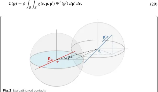
these is located at position P. All rods having their center of gravity at position Q inside the sphere of radius 2L centered at point P could interact with the former. Due to the small size of the considered rods (CNTs), we can assume that the orientation distribu-tion Ψ and concentradistribu-tion φ at posidistribu-tions P and Q coincide.
In fact, because of electronic tunneling effect, the contact between the fibers is not necessarily needed. There is a minimum distance, δ, from which the electrical conduc-tivity occurs. The interaction between rods aligned in directions p and p′ whose centers
of gravity are closer than 2L can be evaluated by a simple geometrical construction as shown in Fig. 2.
The local and directional contact density C(p), when its dependence on the space and time coordinates is omitted, reads
(28) ΨS(x,t, p) = Ψ (x,t, p) + Ψ (x, t, −p) 2 . (29) C(p) = φ B S χ (r, p, p′) ΨS(p′)dp′dr,
where B is the ball of radius 2L centered at point P and where χ(r, p, p′) is a function
equal either to 1 if the distance between the fibers is lower than δ, or to zero otherwise. It can be expected that the conductivity at position x and time t along the direction p scales with the number of contacts φ C(x, t, p)ΨS(x,t, p). Thus the conductivity becomes
local and directional. One can expect that percolation along direction p occurs locally (at position x and time t) when the number of contacts φ C(x, t, p)ΨS(x,t, p) is higher than
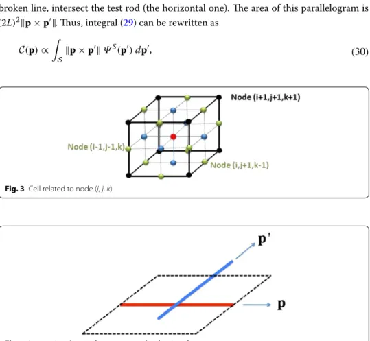
a threshold value T . Lower values imply an infinite local directional electrical resistiv-ity. Thus, percolation could be considered local and directional, allowing us to create a network as described in [28] in which we associate to each node a connexion with each one of its 26 neighbours (Fig. 3). Once we know the local directional resistivity at node (i, j, k) scaling with φ C(x, t, p)ΨS(x,t, p), we can compute the electrical resistances
between node (i, j, k) and each one of its neighbouring nodes, and, using Kirchhoff’s law, analyze the resulting electrical circuit as described in [28].
The microstructure description based on the use of the density of contacts C(p) is very close to that obtained following the rationale proposed by Toll [51, 52] (in continu-ity with the works of Doi and Edwards [53] and Ranganathan and Advani [54]). In our approach, the effect related to the finite diameter of the rods is neglected, but its inclu-sion is straightforward.
The integration involved in Eq. (29) can be understood from the geometrical construc-tion depicted in Fig. 4. It can be noticed that all rods oriented along direction p′ having
their centre of gravity inside the parallelogram of side length 2L, defined by the black broken line, intersect the test rod (the horizontal one). The area of this parallelogram is (2L)2�p × p′�. Thus, integral (29) can be rewritten as
(30)
C(p) ∝
S
�p × p′� ΨS(p′)dp′,
Fig. 3 Cell related to node (i, j, k)
in order to emphasize its resemblance with expressions proposed in the works just mentioned.
The density of contacts C(p) is appropriate because it constitutes a rich description of the microstructure. Its calculation, however, requires knowledge of the distribution function Ψ (p) that is only available when operating at the mesoscale by solving the Fok-ker-Planck equation.
Towards a fully‑macroscopic description
The question arising immediately concerns the existence of an appropriate fully-macro-scopic description.
The simplest proposal consists in defining a tensor L as follows:
which in view of Eq. (30) can be rewritten as
This expression is very close to the interaction tensor b introduced by Ferec et al. [55],
Indeed, we have the equality
As the distribution function ΨS(p) can be approximated from its associated moments
(only the even ones in view of symmetry), as proven in [47], the interaction tensor b can be written from the different orientation tensors aS,(n), n = 2, 4, . . ., where the
super-script S highlights the fact that all of them are associated to the symmetric orientation distribution function ΨS(p). It is easy to verify from the moments’ definition that
This procedure for expressing b as a function of a(2) and a(4) was considered in [56]
where an appropriate expression b = b(a(2), a(4)) was proposed and validated.
This route allows us to finally establish a link between our descriptor L (32) and the standard orientation tensors, which allows for a fully-macroscopic description.
Now, from the knowledge of L, we can obtain the directional properties along direc-tion p by calculating (pT · L · p) p, or equivalently (L : (p ⊗ p)) p.
Another appealing microstructural descriptor could be the second-order tensor J defined such as to verify
In general, such a tensor does not exist, and then the most natural possibility is to enforce this equality is a least-squares sense. Thus, we define the functional F(J),
(31) L = φ S p ⊗ p C(p)ΨS(p)dp, (32) L = β S S p ⊗ p �p × p′� ΨS(p) ΨS(p′)dp dp′. (33) b = S S p ⊗ p �p × p′� ΨS(p) ΨS(p′)dp dp′. (34) L = β · b. (35) aS,(n)= 0 n ∈ [1, 3, 5, . . .] aS,(n)= a(n) n ∈ [2, 4, 6, . . .]. (36) (J : (p ⊗ p)) = C(p).
that should be minimized.
Now, the extremum condition for the functional F(J) yields
or
This expression constitutes a sort of bridge (in a least-squares sense) between macro-scopic and mesomacro-scopic scales. Indeed, knowing L (which can be evaluated from the orientation tensors a(2) and a(4)) and using Eq. (39), we can evaluate the tensor J, from
which we calculate C(p) (in a least-squares sense) from (36).
It is important to recall that, in the least-squares approximation (37), the equality is weighted by the distribution function ΨS(p). This means that more than reproducing
C(p), we are approximating C(p)ΨS(p), which constitutes a better description from the physical point of view, as it combines the potential of a given direction expressed by C(p) with the number Ψ (p) of rods having this orientation.
Numerical results
Evaluating the closure relations
We now evaluate and validate the different closure relations introduced above.
In "Macroscopic description", we derived two frameworks for describing the micro-structure evolution. The first one considers the first moment a(1) such that
It requires two closure relations for expressing the higher-order moments a(2) and a(3) as
a function of a(1).
The second framework involves the first two moments, where Eq. (40) is comple-mented with an equation for the second-order moment:
This second framework requires appropriate closures for the third and fourth-order moments.
In what follows, we consider the richer framework that involves Eqs. (40) and (41) with the order hybrid closure and different choices of that of third order. The fourth-order hybrid closure is given by
(37) F (J) = S ((J : (p ⊗ p)) − C(p))2ΨS(p)dp, (38) J : S p ⊗ p ⊗ p ⊗ p ΨS(p)dp = S p ⊗ p C(p) ΨS(p)dp, (39) φJ : a(4)= L. (40) ˙a(1)= 1 ξL E − a(2)· E + ∇v · a(1)− a(3): ∇v −Dra(1). (41) ˙a(2)= 1 ξL E ⊗ a(1)+ a(1)⊗ E − 2a(3)· E + ∇v · a(2)+ a(2)· (∇v)T− 2 · a(4): ∇v − 2dDr a(2)− I d . (42) a(4),cl=f a(4),qua+ (1 −f )a(4),lin,
where in the 3D case and
where I is the identity tensor.
First, for different orientation distributions Ψ (p, t) coming from the solution of the Fokker-Planck equation for different choices of the velocity and electric fields, we com-pute the third-order moment a(3),FP from Eq. (15) (the superscript FP refers to the
Fok-ker-Planck nature of the solution). We then fit the coefficient α in Eq. (27) in order to minimize the gap (in a least-squares sense) between a(3),FP and a(3),cl,
The best fit was obtained with α adjusted from several numerical experiments as follows: It is easy to verify by taking the trace of both sides of Eq. (41) that d
dttr a(2)(t) = 0,
which implies tr(a(2)(t)) = 1 if the initial condition has a unit trace. However, as the
clo-sure relation (45, 46) does not reproduce exactly a(3), we must check the model
consist-ency by examining if the trace of a(2)(t) remains unitary when integrating Eq. (41) from
an initial condition with unit trace.
In simple shear flow, integration of Eq. (41) with the closure relation (45, 46) yields an unphysical variation of the trace of a(2). This fact can be observed in Fig. 5 which depicts
the evolution of a(2)(t) (on the left) and its trace (on the right) resulting from the
integra-tion of Eq. (41) for planar shear flow vT = (y, 0), ˜E = 1, D
r = 0.1 and an isotropic planar
orientation state.
In relation to Eq. (41), the condition that the third-order closure must satisfy in order to keep the trace constant is 2a(1)· E = 2tr a(3)· E
that can be easily verified
(43) a(4),qua= a(2)⊗ a(2), (44) aijkl(4),lin= −1 35 IijIkl+ IikIjl+ IilIjk + 1 7 a(2)ij Ikl+ aik(2)Ijl+ ail(2)Ijk+ a(2)kl Iij+ ajl(2)Iik+ a(2)jk Iil , (45) a(3),cl= α a(1)⊗ a(1)⊗ a(1) . (46) α = 1.2 − 0.2�a(1)�.
When considering the closure (45) into Eq. (41), we obtain
that must be equal to 2a(1)· E in order to guarantee a constant value of the trace of the
second-order moment. The only possibility is that α in Eq. (45) verifies
from which the third-order moment closure verifying both the symmetry conditions and the model consistency (with respect to the preservation of the unit trace of a(2)) must be
The closure relation (49), however, when considered in the integration of Eq. (41), yields large deviations with respect to the reference solution obtained from the Fokker-Planck solution, as can be seen in Fig. 6 for the same flow conditions as considered previously.
One possibility is to develop richer closures, as for example (26), which in the 2D case reads
With α = µ
tr(a(1)⊗a(1)), Eq. (51) reads
2tr a(3)· E = 2 S tr(p ⊗ p) p · E Ψ (p) dp = (47) 2 S p · E Ψ (p)dp = 2a(1)· E. (48) 2tr a(3),cl· E = 2αtr a(1)⊗ a(1) a1· E, (49) α = 1 tr a(1)⊗ a(1) , (50) a(3),cl= 1 tr a(1)⊗ a(1) a(1)⊗ a(1)⊗ a(1) . (51) a(3),cl= α a(1)⊗ a(1)⊗ a(1) + β(I1⊗ I1⊗ I1) + δ(I2⊗ I2⊗ I2).
from which the trace of Eq. (41) involving the electric contribution gives
where E1 and E2 are the components of E. Considering β = νa(1)1 and δ = υa (1)
2 , the
pre-vious expression can be rewritten as
which must be equal to 2a(1)· E in order to guarantee a constant value of the trace of
the second-order moment. This equality holds if µ + ν + υ = 1. All the possibilities that such richer closures open constitute work in progress whose results will be reported in further works. In what follows, we consider an alternative route.
This alternative route consists in reinterpreting the pragmatic closure (24) by assum-ing that it is in fact a closure of the tensor product a(3)· E, that is
With the second moment closure verifying the normality property tr a(2),cl = 1, as
ensured for example by Eq. (21), we have the equality
that ensures the model consistency (unit trace).
Thus, in what follows, the retained closures of the third-order terms in Eqs. (40) and (41) are respectively
and
In the forthcoming numerical examples, we use Eqs. (40) and (41) with the fourth-order hybrid closure (42) and the third-order closures (57) and (58). We first consider planar flows characterized by a velocity gradient of the general form
and different values of the diffusion coefficient.
(52)
a(3),cl= µ a
(1)⊗ a(1)⊗ a(1)
tr(a(1)⊗ a(1)) + β(I1⊗ I1⊗ I1) + δ(I2⊗ I2⊗ I2),
(53) 2tr a(3)· E ≈ 2tr a(3),cl· E = 2 µa(1)· E + βE1+ δE2 , (54) 2tr a(3)· E = 2(µ + ν + υ) a(1)· E, (55) a(3)· E cl= a(2),cl⊗ a(1) · E = a(2),cl(a(1)· E). (56) tr a(3)· E cl=tr a(2),cl (a(1)· E) = a(1)· E, (57) a(3): ∇v cl= a(1)(a(2),cl: ∇v), (58) a(3)· E cl= a(2),cl(a(1)· E). (59) ∇v = Gxx Gxy 0 0 Gyy 0 0 0 0 ,
In all cases, the Fokker-Planck equation (9) is solved for the orientation distribution Ψ (p,t) by means of the PGD. The initial orientation distribution is assumed isotropic. From Ψ (p, t), the first and second-order moments a(1),FP(t) and a(2),FP(t) are calculated,
respectively from Eqs. (13) and (14). This procedure does not involve any closure rela-tion. The solutions a(1),FP(t) and a(2),FP(t) can thus be considered as reference solutions.
The same moments are now computed via Eqs. (40) and (41) using closure approxi-mations. When integrating Eq. (40) to obtain a(1)(t), we take the second-order moment
from the solution of Eq. (41) and the third-order moment is approximated by using the closure (57). When integrating Eq. (41) to obtain a(2)(t), we use the closure (58) for the
third-order moment and the standard hybrid closure (42) for the fourth-order moment. We consider both simple shear and extensional flows for evaluating the accuracy of the resulting closed macroscopic description:
– Shear flow: Gxx= 0, Gxy= 1 and Gyy= 0 with Dr= 0.1 and Dr = 0.01. – Extensional flow: Gxx= 1, Gxy= 0 and Gyy= −1 with Dr = 0.1 and Dr = 0.01.
In Figs. 7 and 8, the approximate closure solutions a(1) and a(2) are compared with the
reference solutions a(1),FP and a(2),FP obtained from the direct solution of the
Fokker-Planck equation. Agreement is in general quite satisfactory, but the development of even more precise closures will require a considerable amount of work.
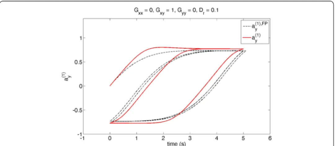
It is well known that closure relations can induce artifacts, as for example the disap-pearance of hysteric behaviour in reversal flows. To check the model response in such conditions, we apply a simple shear flow defined by vT = ( ˙γy, 0, 0) for t ∈ [0, T = 5s];
the flow is reversed for t ∈ [T, 2T] by changing the sign of ˙γ, and it is again reversed in subsequent time intervals. In other words, the shear flow is reversed at times t = nT, n = 1, 2, . . .
We see in Fig. 9 that the closure solution a(1) constitutes a reasonable approximation
of the reference solution, again computed from the orientation distribution solution of the associated Fokker-Planck equation. In order to appreciate this more clearly, Fig. 10
compares the component a(1)
y of both solutions. Finally, we compare in Fig. 11 the planar
component of a(2) and a(2),FP. All these results show that the proposed closure relations
remain quite reasonable and do not introduce unphysical behaviours. Parametric solution of the Fokker‑Planck equation
When controlling the applied flow and electric fields, one could require many solutions of the model in order to reach optimal conditions with respect to an output of inter-est. In these circumstances, the parametric solution of the model would be extremely
Fig. 8 (Top) First and second moments for Dr= 0.1 and (bottom) first and second moments for Dr= 0.01
valuable. As the PGD parametric solution of the Fokker-Planck equation is performed offline and only once, it is indeed well worth the effort [44], despite of the necessity of solving a high-dimensional problem, involving the physical coordinates (space and time), the conformational coordinates (orientation) and a number of extra-coordinates (model parameters) as described in "Parametric solutions of the Fokker-Planck equation".
In what follows, we consider a homogeneous simple shear flow vT = ( ˙γy, 0, 0), ˙γ = 1.
Its homogeneity avoids the dependence of the orientation distribution function Ψ on the space coordinates x. We assume planar orientation, with a single conformational coor-dinate to describe it, i.e. the angle θ with respect the x−coorcoor-dinate axis. An electric field of intensity E is applied along the y−coordinate axis, i.e. E = Eiy (with iy the unit vector
defining the y−coordinate axis direction). In this section, E refers to the effective electric field denoted by ˜E in "Parametric solutions of the Fokker-Planck equation".
Thus, the four-dimensional parametric solution Ψ (t, θ, Dr,E) of the Fokker-Planck
equation (7) is sought in the separated form
(60) Ψ (t, θ , Dr,E) ≈ i=N i=1 Fit(t) · Fiθ(θ ) ·FiD(Dr) ·FiE(E). Fig. 10 Solution a(1)
y versus a(1),FPy in simple shear flow with regular flow reversals
Fig. 11 Solution a(2)
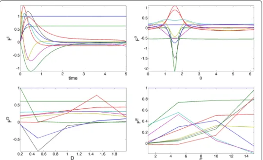
Figure 12 depicts the different functions involved in the separated representa-tion (60). Finally, Fig. 13 shows the reconstructed parametric steady state solution Ψ (t → ∞, θ , Dr,E).
For more details on the practical implementation of the PGD for solving parametric PDE’s, see [44–46].
Evaluating interaction descriptors
Finally, we check whether the different interaction descriptors discussed in "Description of the rod network" perform as expected.
First, given the two planar orientation distributions shown in Fig. 14, we compute the density of contacts C(θ) given by Eq. (29) and the one given by Toll [51, 52]. Both results
Fig. 12 PGD modes involved in the separated representation of the parametric solution Ψ (t, θ, Dr, E):
(top-left) Ft
i(t); (top-right) Fiθ(θ ); (bottom-left) FiD(Dr) and (bottom-right) FiE(E)
are compared in Fig. 15. We observe an excellent agreement despite of some hypotheses introduced in our approach (related to the assumption of a vanishing rod diameter).
As expected, Fig. 16 shows the perfect agreement between the scaled Ferec interaction tensor b, Eq. (33), and the one that we proposed above, L, Eq. (31).
Finally, we discussed in "Towards a fully-macroscopic description" the use of ten-sor J as an interaction descriptor in order to fit in a least-squares sense the density of contacts. The least-squares being weighted by the distribution function Ψ, the resulting directional information J : (p ⊗ p) is closer to CΨ than to C, as can be noticed in Fig. 17.
Fig. 14 Two orientation distributions for a large (left) and a smaller (right) diffusion coefficient
Fig. 15 Directional density of contacts: C(p) versus Toll’s model
Conclusions
In this work, we have revisited the microstructural kinematics of electrically conductive rods immersed in a flowing suspension to which an electric field is applied. The evolu-tion equaevolu-tion for the microscopic rod orientaevolu-tion was derived by considering standard balances of forces and moments. These kinematics were then introduced into a meso-scopic description based on the Fokker-Planck equation, whose parametric solution was formulated within the separated representation framework at the heart of the method of Proper Generalized Decomposition. The mesoscopic description was coarsened one step further in order to derive a fully macroscopic description based on the use of the first or the first two moments of the orientation distribution. Both approaches require the use of appropriate closure relations. In the present work, we proposed consistent closures for the third-order orientation tensor, which despite being non optimal produce
results that are in reasonable agreement with reference solutions obtained directly from the Fokker-Planck description.
On the other hand, prediction of the electrical properties of the suspension as a whole requires the quantification of the rod interaction. We quantified the directional con-ductivity by calculating the directional density of contacts that depends on the orien-tation distribution and the local rod concentration. This approach, already considered in our former work [28], requires however the mesoscopic calculation of the orienta-tion distribuorienta-tion. In this work, we proposed an alternative fully-macroscopic route. For that purpose, we defined an interaction tensor L which by construction is equivalent to the interaction tensor proposed by Ferec in [55]. As the latter can be approximated with reasonable accuracy from the orientation tensors of even order, a fully macroscopic approach is thus finally obtained.
Author details
1 GeM UMR CNRS‑Centrale Nantes, 1 rue de la Noe, 44300 Nantes, France. 2 Arts et Métiers ParisTech, 2 Boulevard du Ron‑
ceray, BP 93525, 49035 Angers cedex 01, France. 3 UMSSDT, ENSIT, Universit de Tunis, 5, avenue Taha‑Hussien, Montfleury,
1008 Tunis, Tunisia. 4 ICTEAM, Université catholique de Louvain, Bat. Euler, Av. Georges Lemaitre 4, 1348 Louvain‑la‑Neuve,
Belgium.
Competing interests
The authors declare that they have no competing interests.
References
1. Coleman JN, Khan U, Gunko YK. Mechanical reinforcement of polymers using carbon nanotubes. Adv Mater. 2006;18:689–706.
2. Xu YS, Ray G, Abdel‑Magid B. Thermal behavior of single‑walled carbon nanotube polymer‑matrix composites. Compos Part A‑Appl Sci Manuf. 2006;37:114–21.
3. Ounaies Z, Park C, Wise KE, Siochi EJ, Harrison JS. Electrical properties of single wall carbon nanotube reinforced polyimide composites. Compos Sci Technol. 2003;63:1637–46.
4. Ma A, Chinesta F, Mackley M. The rheology and modelling of chemically treated Carbon Nanotube suspensions. J Rheol. 2009;53(3):547–73.
5. Ma A, Chinesta F, Ammar A, Mackley M. Rheological modelling of Carbon Nanotube aggregate suspensions. J Rheol. 2008;52(6):1311–30.
6. Hwang TY, Kim HJ, Ahn Y, Lee JW. Influence of twin screw extrusion processing condition on the properties of polypropylene/multi‑walled carbon nanotube nanocomposites. Korea‑Aust Rheol J. 2010;22:141–8.
7. Villmow T, Pegel S, Poetschke P, Wagenknecht U. Influence of injection molding parameters on the electrical resistiv‑ ity of polycarbonate filled with multi‑walled carbon nanotubes. Compos Sci Technol 2008;68:777–89.
8. Obrzut J, Douglas JF, Kharchenko SB, Migler KB. Shear‑induced conductorinsulator transition in melt‑mixed polypropylene‑carbon nanotube dispersions. Phys Rev B. 2007;76:195420.
9 Bauhofer W, Schulz SC, Eken AE, Skipa T, Lellinger D, Alig I, Tozzi EJ, Klingenberg DJ. Shearcontrolled electrical conductivity of carbon nanotubes networks suspended in low and high molecular weight liquids. Polymer. 2010;51:5024–7.
10. Eken AE, Tozzi EJ, Klingenberg DJ, Bauhofer W. A simulation study on the effects of shear flow on the microstructure and electrical properties of carbon nanotube/polymer composites. Polymer. 2011;52:5178–85.
11. Kashiwagi T, Fagan J, Douglas JF, Yamamoto K, Heckert AN, Leigh SD, Obrzut J, Du F, Lin‑Gibson S, Mu M, Winey KI, Haggenmueller R. Relationship between dispersion metric and properties of PMMA/SWNT nanocomposites. Polymer. 2007;48:4855–66.
12. Haggenmueller R, Fischer JE, Winey KI. Single wall carbon nanotube/polyethylene nanocomposites: nucleating and templating polyethylene crystallites. Macromolecules. 2006;39:2964–71.
13. Abbasi S, Carreau PJ, Derdouri A. Flow induced orientation of multiwalled carbon nanotubes in polycarbonate nanocomposites: rheology, conductivity and mechanical properties. Polymer. 2010;51:922–35.
14. Alig I, Skipa T, Lellinger D, Bierdel M, Meyer H. Dynamic percolation of carbon nanotube agglomerates in a polymer matrix: comparison of different model approaches. Phys Status Solidi B Basic Solid State Phys. 2008;245:2264–7. 15. Alig I, Potschke P, Lellinger D, Skipa T, Pegel S, Kasaliwal GR, Willmow T. Establishment, morphology and properties of
carbon nanotube networks in polymer melts. Polymer. 2012;53:4–28.
16. Bauhofer W, Kovacs JZ. A review and analysis of electrical percolation in carbon nanotube polymer composites. Compos Sci Technol. 2009;69:1486–98.
17. Kharchenko SB, Douglas JF, Obrzut J, Grulke EA, Migler KB. Flow‑induced properties of nanotube‑filled polymer materials. Nat Mater. 2004;3:564–8.
18. Ma A, Mackley M, Chinesta F. The microstructure and rheology of carbon nanotube suspensions. Int J Mat Forming. 2008;2:75–81.
19. Schueler R, Petermann J, Schulte K, Wentzel HP. Agglomeration and electrical percolation behavior of carbon black dispersed in epoxy resin. J Appl Polym Sci. 1997;63:1741–6.
20. Abisset‑Chavanne E, Mezher R, Le Corre S, Ammar A, Chinesta F. Kinetic theory microstructure modeling in concen‑ trated suspensions. Entropy. 2013;15:2805–32.
21. Abisset‑Chavanne E, Chinesta F, Ferec J, Ausias G, Keunings R. On the multiscale description of dilute suspensions of non‑Brownian rigid clusters composed of rods. J Non‑Newtonian Fluid Mech. 2015;222:34–44.
22. Chinesta F. From single‑scale to two‑scales kinetic theory descriptions of rods suspensions. Archiv Comp Methods Eng. 2013;20(1):1–29.
23. Petrich MP, Koch DL, Cohen C. An experimental determination of the stress‑microstructure relationship in semi‑ concentrated fiber suspensions. J Non‑Newtonian Fluid Mech. 2000;95:101–33.
24. Dalmas F, Dendievel R, Chazeau L, Cavaille JY, Gauthier C. Carbon nanotube‑filled polymer composites. Numeri‑ cal simulation of electrical conductivity in three‑dimensional entangled fibrous networks. Acta Materialia. 2006;54:2923–31.
25. Rahatekar SS, Hamm M, Shaffer MSP, Elliott JA. Mesoscale modeling of electrical percolation in fiber‑filled systems. J Chem Phys. 2005;123:134702.
26. Seidel GD, Puydupin‑Jamin AS. Analysis of clustering, interphase region, and orientation effects on the electri‑ cal conductivity of carbon nanotube‑polymer nanocomposites via computational micromechanics. Mech Mat. 2011;43(12):755–74.
27. Seidel GD, Lagoudas DC. A micromechanics model for the electrical conductivity of nanotube‑polymer nanocom‑ posites. J Comp Mat. 2009;43(9):917–41.
28. Perez M, Abisset‑Chavanne E, Barasinski A, Ammar A, Chinesta F, Keunings R. Towards a kinetic theory description of electrical conduction in perfectly dispersed CNT nanocomposites. Chapter in Rheology of Non‑Spherical Particle Suspensions, ISTE‑Wiley (In press).
29. Jeffery GB. The motion of ellipsoidal particles immersed in a viscous fluid. Proc R Soc London. 1922;A102:161–79. 30. Bird RB, Crutiss CF, Armstrong RC, Hassager O. Dynamic of polymeric liquid, Volume 2: Kinetic Theory, John Wiley
and Sons, 1987.
31. Doi M, Edwards SF. The theory of polymer dynamics. Oxford: Clarendon Press; 1987.
32. Keunings R. Micro‑macro methods for the multiscale simulation of viscoelasticowusing molecular models of kinetic theory. Rheology Reviews. Binding DM, Walters K (eds), British Society of Rheology 2004.
33. Petrie C. The rheology of fibre suspensions. J Non‑Newtonian Fluid Mech. 1999;87:369–402.
34. Folgar F, Tucker Ch. Orientation behavior of fibers in concentrated suspensions. J Reinf Plast Comp. 1984;3:98–119. 35. Ammar A, Mokdad B, Chinesta F, Keunings R. A new family of solvers for some classes of multidimensional partial
differential equations encountered in kinetic theory modeling of complex fluids. J Non‑Newtonian Fluid Mech. 2006;139:153–76.
36. Ammar A, Mokdad B, Chinesta F, Keunings. A new family of solvers for some classes of multidimensional partial differential equations encountered in kinetic theory modeling of complex fluids. Part II.transient simulation using space‑time separated representations. J Non‑Newtonian Fluid Mech. 2007;144:98–121.
37. Ammar A, Normandin M, Daim F, Gonzalez D, Cueto E, Chinesta F. Non‑incremental strategies based on separated representations: applications in computational rheology. Commun Math Sci. 2010;8(3):671–95.
38. Ammar A, Normandin M, Chinesta F. Solving parametric complex fluids models in rheometric flows. J Non‑Newto‑ nian Fluid Mech. 2010;165:1588–601.
39. Chinesta F, Ammar A, Cueto E. Recent advances and new challenges in the use of the Proper Generalized Decom‑ position for solving multidimensional models. Archiv Comput Methods Eng. 2010;17(4):327–50.
40. Chinesta F, Ladeveze P, Cueto E. A short review in model order reduction based on Proper Generalized Decomposi‑ tion. Archiv Comput Methods Eng. 2011;18:395–404.
41. Mokdad B, Pruliere E, Ammar A, Chinesta F. On the simulation of kinetic theory models of complex fluids using the Fokker‑Planck approach. Appl Rheol. 2007;17/2(26494):1–14.
42. Mokdad B, Ammar A, Normandin M, Chinesta F, Clermont JR. A fully deterministic micro‑macro simulation of com‑ plex flows involving reversible network fluid models. Math Comp Simul. 2010;80:1936–61.
43. Pruliere E, Ammar A, El Kissi N, Chinesta F. Recirculating flows involving short fiber suspensions: numerical difficulties and efficient advanced micro‑macro solvers. Archiv Comp Methods Eng State Art Rev. 2009;16:1–30.
44. Chinesta F, Keunings R, Leygue A. The Proper Generalized Decomposition for advanced numerical simulations. A primer. Springerbriefs: Springer; 2014.
45. Chinesta F, Ammar A, Leygue A, Keunings R. An overview of the Proper Generalized Decomposition with applica‑ tions in computational rheology. J Non Newtonian Fluid Mech. 2011;166:578–92.
46. Chinesta F, Leygue A, Bordeu F, Aguado JV, Cueto E, Gonzalez D, Alfaro I, Ammar A, Huerta A. Parametric PGD based computational vademecum for efficient design, optimization and control. Archiv Comput Methods Eng. 2013;20(1):31–59.
47. Advani S, Tucker Ch. The use of tensors to describe and predict fiber orientation in short fiber composites. J Rheol. 1987;31:751–84.
48. Advani S, Tucker Ch. Closure approximations for three‑dimensional structure tensors. J Rheol. 1990;34:367–86. 49. Dupret F, Verleye V. Modelling the flow of fibre suspensions in narrow gaps. In: Siginer DA, De Kee D, Chabra RP, edi‑
tors. Advances in the flow and rheology of Non‑Newtonian fluids. Rheology Series: Elsevier; 1999. p. 1347–98. 50. Kroger M, Ammar A, Chinesta F. Consistent closure schemes for statistical models of anisotropic fluids. J Non‑Newto‑
nian Fluid Mech. 2008;149:40–55.
51. Toll S. Note: on the tube model for fiber suspensions. J Rheol. 1993;37/l:123–5. 52. Toll S. Packing mechanics of fiber reinforcements. Polymer Eng Sci. 1998;38(8):1337–50.
53. Doi M, Edwards SF. Dynamics of rod‑like macromolecules in concentrated solution. Part 1. J Chem Soc Faraday Trans. 1978;2(74):560–70.
54. Ranganathan S, Advani SG. Fiber‑fiber interactions in homogeneous flows of nondilute suspensions. J Rheol. 1991;35/ 8:1499–522.
55. Ferec J, Ausias G, Heuze M‑C, Carreau P. Modeling fiber interactions in semi concentrated fiber suspensions. J Rheol. 2009;53(1):49–72.
56. Ferec J, Abisset‑Chavanne E, Ausias G, Chinesta F. On the use of interaction tensors to describe and predict rod interactions in rod suspensions. Rheol Acta. 2014;53:445–56.