Crisis and Income Distribution:
A Micro-Macro Model for Indonesia
Anne-Sophie Robilliard*, Francois Bourguignon°, and Sherman Robinson*1
March 2001
Draft for Comments – Preliminary Results
Abstract
In this paper, a novel approach is implemented to quantify the effects on poverty and inequality of the financial crisis that hit Indonesia in 1997. It relies on the combination of a microsimulation model and a standard CGE model. These two models are used in a sequential fashion in order to simulate the impact of the crisis and to examine counterfactual policy scenarios. The CGE model is based on a Social Accounting Matrix with 38 sectors and 15 factors of production. It captures structural features of the economy, including binding macro constraints, and incorporates general equilibrium effects. The microsimulation model is based on a detailed representation of the real income generation mechanism at the household level. It captures household heterogeneity in terms of income sources, area of residence, demographic composition, endowment in human capital, and consumption preferences. It is based on a sub-sample of 9,800 households from the 1996 SUSENAS survey. This framework allows us to decompose the effects of the financial crisis as well as to compare the impact of introducing alternative social policy packages during the crisis such as food subsidies, household transfers or public work programs.
* International Food Policy Research Institute, Washington, D.C. ° The World Bank, Washington, D.C.
1
We are very grateful to Indonesia’s Badan Pusat Statistik (BPS) for making the data available. We thank Vivi Alatas for help with the data and programming. We would also like to thank Benu Bidani, Dave Coady, Gaurav Datt, Tamar Manuelyan Atinc, and Emmanuel Skoufias, for comments and useful discussions, as well as seminar participants at IFPRI and the World Bank. All errors are our own.
1. Introduction
Since 1998, the social impact of the financial crisis that hit Indonesia has been an important subject of concern for both policy makers and financial institutions. One year after the crisis, several
estimates of the effects of the crisis on the poor and vulnerable groups in Indonesian society were
published—the first in July 1998 by the World Bank (World Bank, 1998), the second by the
Indonesian Board of Statistics (CBS, 1998), and the third by the International Labour Organization (ILO, 1998). The World Bank report argued that if real GDP declined by 12% in 1998, it would
push the incidence of poverty up to 14.1% of the population in 1999 from a level of 10.1% in
mid-1997. Estimates from the ILO and CBS projected a four to five fold increase of the poverty
head-count, from 11.3% in 1996 up to 39.9% for mid-1999 (CBS, 1998) and 48.2% for end-1998 (ILO, 1998), and a six fold increase up to 66.3% for the end of 1999 (ILO, 1998).2 In a recent study based on data collected in the National Labor Force Surveys (Sakernas) from August 1997
through 1998, Manning (2000) suggests that the shock was not as bad as some had predicted, but
had led to important adjustments on the labor markets. Finally, recent estimates published by the World Bank (Suryahadi et al., 2000), based on a comparison of the poverty level between two
Susenas surveys, show that between 1996 and 1999 the poverty head-count rose by 66.8%, from
9.75% to 16.27%.
This last study is typical of most existing studies of the distributive effects of macroeconomic
shocks, relying on a comparison of the distribution before and after the shock. This approach suffers
well-known drawbacks. In the case of Indonesia, while the dramatic increases in poverty should be at least partly attributable to the financial crisis, the “before-after” approach does not allow
disentangling the effects of the crisis per se from other exogenous shocks such as the El Nino drought
that hit Indonesia in 1997. Another common approach is based on macro models with some degree
of disaggregation of the household sector (Dervis et al., 1982 ; Adelman and Robinson, 1989). While the use of an empirical modeling framework makes it possible to analyze counterfactual
2
scenarios and decompose the specific effects of various shocks, the models are generally too
aggregated to estimate changes in the overall size distribution of income.3
In this paper, we use a new approach to quantify the effects of the crisis on poverty and
inequality, combining a microsimulation model with a standard CGE model. These two models are
used in a sequential fashion in order to simulate the impact of the crisis and to examine counterfactual
policy scenarios. The CGE model is based on a Social Accounting Matrix with 38 sectors and 15 factors of production. It captures structural features of the economy, including binding macro
constraints, and incorporates general equilibrium effects. The microsimulation model is based on a
sub-sample of the Susenas survey for the year 1996 and simulates occupational choice behavior for
more than 33,000 individuals.4 The two models are treated separately. The macro CGE model communicates with the microsimulation model by generating a vector of prices, wages, and aggregate
employment variables. The structure and the functioning of labor markets thus play an important role.
This overall framework generates poverty and inequality measures from the microsimulation model
based on the full household survey, without requiring any prior assumptions regarding within-group income distributions.
The paper is organized as follows. In Section 2, the microsimulation model is described. In Section 3, the CGE model is described. Scenarios and simulation results are presented in Section 4.
2. The Microsimulation Model
The essence of the microsimulation approach is to model in detail the behavior of individual
firms or households observed at the micro level. The approach was developed in recent years using
the growing body of micro survey data and the capacity of computers to retain large amounts of information. The microsimulation model for Indonesia incorporates occupational choices for more
3
In this framework, the overall size distribution can be generated given strong assumptions about the within group distributions (Adelman and Robinson, 1978), but there are still serious aggregation issues.
4
The SUSENAS sample used is the same as the one used by Alatas and Bourguignon (1999) for a study of the evolution of the distribution of income during Indonesian fast growth 1980-1996. The design of the microsimulation framework draws partly from this previous work.
than 33,000 individuals aged 10 years or more, and generates household income for more than
9,800 households. Income sources include earnings from wage work as well as income from
self-employment. The model captures the heterogeneity of individuals in terms of human capital
endowment and occupational choice preferences, and captures the heterogeneity of households in terms of sources of income and demographic composition. We start by presenting a simple analytic
version of model.
The model is based on a detailed representation of the real income generation mechanism at
the household level. It thus relies on the estimation of earning functions for wage workers, segmented
into several groups by skill, gender, and area of residence; profit functions for self-employed
workers in the farm and non-farm sectors; and models of individual occupational choice between inactivity, wage work, or self-employment. In addition, total household income is deflated by a
household specific price index that depends on the prices of the various consumption goods and the
observed budget shares in each household. The link with the CGE part of the analysis is provided by
wage levels in the various markets for wage labor, value added prices for the self-employed, total employment for the various groups of wage workers and farm and non-farm self-employment, and
finally the vector of consumption prices. For each set of values of these variables delivered by the
CGE part of the overall model, the micro-simulation module computes changes in earnings,
self-employment income, individual occupational choices, and the price deflator of nominal household income. The microsimulation model is solved so that it generates equilibrium values of households
labor supplies such that aggregate changes are consistent with the results from the CGE model.
This section briefly describes the specification of the household income generation model and
then focuses on the way the consistency between micro-simulation and the predictions of the CGE
model is achieved. A more detailed discussion of the household model and its various components
may be found in Alatas and Bourguignon (2000).5
5
A more general discussion of the methodology may be found in Bourguignon, Ferreira and Lustig (1998) and Bourguignon, Fournier and Gurgand (2001). For a general discussion of the link between CGE modeling and micro-unit household data see Plumb (2001).
The household income function used in the case of Indonesia may be summarized by the
following set of equations:
( ) ( ) α β = + + mi g m i mi g m i m i L o g w x v (1) ( ) ( ) ( ) γ δ λ η = + + + m f m m f m f m m m Log y Z N (2) 0 1 1 ( 0) = = + > +
∑
m k m mi m m m m i m Y w IW y Ind N y P (3) 1 = =∑
K m mk k k P s p (4) ( ) ( ) ( ) ( ) [ (0, )] = w + w + w > s + s + s mi h mi mi h mi mi h mi mi h mi mi IW Ind a z b u Sup a z b u (5) ( ) ( ) ( ) ( ) 1 [ (0, )] = =∑
km s + s + s > w + w + w m h mi mi h mi mi h mi mi h mi mi i N Ind a z b u Sup a z b u (6)The first equation expresses the (log) wage of member i of a household m, with km members at working age, as a function of his/her personal characteristics, x. The latter essentially include age,
schooling level, and region. The residual term, vmi, describes the effects of unobserved earning
determinants. This earning function is defined separately on various “segments” of the labor market
defined by gender, skill (less than secondary or more than primary), and region (urban/rural). Thus
g(mi) is an index function and indicates the labor market segment to which member i in household m
belongs.
The second equation is the profit function associated with self-employment, or small
entrepreneurial activity. Income is now defined at the household level. It depends on the number Nm of household members actually involved in that activity and on some household characteristics. These
include region of residence, the age and schooling of the household head, and land size for farmers. The residual term, ηm, describes the effects of unobserved determinants of self-employment profits. A separate function is used depending on whether the household is involved in farm or non-farm
activity. This is exogenous and defined by whether the household has access to land or not, as
represented by the index function f(m).
The third equation is an accounting identity that defines total household real income, Ym, as
the sum of wage income of its members, profit from self-employment, and (exogenous) non-labor
income, y0. In this equation, the notation IWmi stands for a dummy variable that is equal to unity if
member i is a wage worker and zero otherwise. Thus wages are summed over only those members actually engaged in wage work. Likewise, profit from self-employment has to be taken into account
only if there is at least one member of the household engaged in self-employment activity (Nm>0). Total income is then deflated by a household specific consumer price index, Pm, which is derived from the observed budget shares of household m and the price, p, of the various consumption goods in the model (equation 4).
The last two equations represent the occupational choice made by household members. This choice is discrete. Each individual has to choose from three alternatives : being inactive, being a wage
worker, or being self-employed. The alternative with the highest utility is selected. The utility
associated with the first alternative is arbitrarily set to zero, whereas the utility of being a wage
worker or a self-employed are linear functions of a set of individual and household characteristics, zmi. The intercept of these functions has a component, aw or as, that is common to all individuals and an idiosyncratic term, umi, which stands for unobserved determinants of occupational choices. The coefficients of individual characteristics zmi, bw, or bs, are common to all individuals. However, they may differ across demographic groups indexed by h(mi). For instance, the occupational choice behavior of household heads may be different from that of spouses, or that of female children may be
different from that of male. The constants may also be demography specific.
Given this specification of the utility of the various alternatives on the labor market, an
individual will prefer wage work if the utility associated with that activity is higher than that associated
with the two other activities. This is the meaning of equation (4). Likewise, the number of
employed workers in a household is the number of individuals for whom the utility of self-employment is higher than that of the two alternatives, as represented in (5).
The model is now complete. Overall, it defines the total real income of a household as a
non-linear function of the observed characteristics of household members (xmi and zmi), some characteristics of the household (Zm), its budget shares (sm), and unobserved characteristics (vmi, ηm, uwmi, and usmi). This function depends on five sets of parameters. The parameters in the earning functions (αg and βg), for each labor market segment, g; the parameters of the profit functions (γf, δf, and λf) for the farm or non-farm sector f; the parameters in the utility of the various alternative occupational choices (awh , bwh, ash and bsh), for the various demographic groups h: and the vector of prices (p). We shall see later that it is through all these parameters that the results of the CGE part of the model may be transmitted to the micro-simulation module.
The microsimulation model gives a rather complete description of household income generation mechanisms by focusing on both earning and occupational choice determinants. However,
a number of assumptions about the functioning of the labor market are incorporated in this
specification. The fact that labor supply is considered as a discrete choice between inactivity and full
time work for wages or for self-employment profits within the household calls for two sets of remarks. First, the assumption that individuals either are inactive or work full time is justified
essentially by the fact that no information on working time is available in the micro data base used to
estimate the benchmark set of the model's coefficients. 6 Practically, this implies that estimated individual earning functions (1) and profit functions (2) may incorporate some labor supply dimension. Second, distinguishing between wage work and self-employment is implicitly equivalent to
assuming that the Indonesian labor market is imperfectly competitive. If this were not the case, then
returns to labor would be the same in both types of occupation and self-employment income would
be different from outside wage income only because it would incorporate the returns to non-labor assets being used. The specification that has been selected is partly justified by the fact that all assets
used in self-employment are not observed, so that one cannot distinguish between self-employment
6
The occupational choice model that has been estimated comprises an additional alternative, which corresponds to individuals who report both wage work and self-employment. Even in that case, however, actual working times are not known.
income due to labor and that due to other assets. But it is also justified by the fact that the labor
market may be segmented in the sense that labor returns are not equalized across wage work and
self-employment. There may be various reasons for this. On the one hand, there may be rationing in
the wage labor market. People unable to find a job as a wage worker move into self-employment, which is a kind of shelter. On the other hand, there may be externalities that make working within
and outside the household imperfect substitutes. All these interpretations are fully consistent with the
way in which the labor-market is represented in the CGE part of the model.7
As already mentioned, the benchmark simulation of the model requires previous estimation
work. This is necessary to have an initial set of coefficients (αg, βg, γf, δf, λf, awh, bwh, ash, bsh) as well as an estimate of the unobserved characteristics that enter the earning and profit functions, or the utility of the various occupational alternatives (vmi, ηm, uwmi , usmi). The data base consists of a sample of 9,800 households and 28,000 individuals drawn from the “income and saving” module of
Indonesia's 1996 SUSENAS household survey. The coefficients of earning and profit functions and
the corresponding residual terms are obtained by straight ordinary least square estimation on wage earners and households with some self-employment activity.8 For individuals at working age (i.e. 15 years and older) who are not observed as wage earners in the survey, unobserved characteristics,
vmi, are generated by drawing random numbers from the distribution that is observed for actual wage earners. The same is done with ηm for those households who are not observed as self-employed in the survey but might get involved in that activity in a subsequent simulation.
Parameters of occupational utility functions were obtained through the estimation of a multi-logit model, thus assuming that the residual terms (uwmi , usmi) were distributed according to the double exponential law. The estimation was done for all individuals of working age separately for
household heads, spouses, and other family members. The set of explanatory variables, zmi, included
7
Note that the rationing interpretation of the functioning of the labor market is somewhat inconsistent with the formulation of the occupational choice model (5)-(6) in terms of the 'utility' of various alternatives. With rationing , these clearly should be 'constrained utilities'.
8
Correction for selection biases did not lead to significant changes in the coefficients of these equations and was thus dropped.
not only the socio-demographic characteristics of the individual, but also the average characteristics
of the other members in the household and the size and composition of the household. In addition, it
included the occupational status of the head, and possibly his/her individual earning, for spouses and
other household members. For all individuals, values of the residual terms (uwmi , usmi) were drawn randomly in a way consistent with observed occupational choices. For instance, residual terms for a
wage earner should be such that :
( ) ˆ( ) ( ) ˆ( )
ˆw + w + w > (0,ˆs + s + s )
h mi mi h mi mi h mi mi h mi mi
a z b u Sup a z b u
where the ^ notation corresponds to multi-logit coefficient estimates.
Results of these various estimation procedures are given in Appendix A. For lack of space, we do not repeat the discussion that may be found in Alatas and Bourguignon (2000). Note that the
CPI equation (4) does not call for any estimation work since it is directly defined on observed
household budget shares.
We now describe how the link is made with the CGE part of the model and how the effects
of macro-economic shocks and policies are simulated on each household in the data base. The
principle of these simulations is extremely simple. It consists of associating macro-economic shocks and policies simulated in the CGE part of the model to changes in the set of coefficients of the
household income generation model (1)-(6). This association has to be done in a consistent way.
Consistency, or equilibrium, requires that: (1) changes in average earnings in the micro-simulation
module must be equal to changes in wage rates in the CGE model for each segment of the market for wage labor; (2) changes in self-employment income in the micro-simulation module must be equal to
changes in informal sector income per worker in the CGE model; (3) changes in the number of wage
workers and self-employed by labor-market segment in the micro-simulation module must match
those same changes in the CGE model, (4) and changes in the consumption price vector, p, must be consistent with the CGE model.
The calibration of the CGE model is done in such a way that the preceding three sets of consistency requirements are satisfied in the benchmark simulation. Let EG be the employment level
in the G segment of the wage labor market, wG the corresponding wage rate, SG the number of self-employed in the same segment and IF the total self-employment household income in informal sector F (farm and non-farm). Finally, let q be the vector of prices for consumption goods in the CGE
model. Consistency between the micro data base and the benchmark run of the CGE model is described by the following set of constraints.
( ) ( ) ( ) ( ) , ( ) ( ) ( ) ( ) ( ) , ( ) ( ) ˆ ˆ ˆ ˆ ˆ ˆ [ . (0, . ) ] ˆ ˆ ˆ ˆ ˆ ˆ [ . (0, . ) ] ˆ ˆ ˆ ˆ ( . ). [ w w w s s s h m i mi h mi mi h mi mi h m i mi G m i g mi G S S S w w w h m i mi h mi mi h mi mi h m i mi G m i g mi G w G mi G mi h m i Ind a z b u Sup a z b u E Ind a z b u Sup a z b u S Expα x β v Ind a z = = + + > + + = + + > + + = + + +
∑ ∑
∑ ∑
( ) ( ) ( ) , ( ) , ( ) ( ) ( ) ( ) ( ) ˆ ˆ ˆ ˆ ˆ . (0, . ) ] ˆ ˆ ˆ ˆ ˆ ( . . ). ( 0) ˆ ˆ ˆ [ ˆ . ˆ (0, ˆ . ˆ ) ] w w s s s mi h mi mi h mi mi h m i mi G m i g mi G F m F F m m m F m f m F S S S w w w m h m i mi h mi mi h mi mi h m i mi i b u Sup a z b u w Exp Z N Ind N Iwith N Ind a z b u Sup a z b u
γ δ λ η = = + > + + = + + + > = = + + > + +
∑ ∑
∑
∑
In these equations, the ^ notation refers to the results of the estimation procedure described
above. The predicted occupational choices, earnings, and self-employment income that appear in these equations are identical for all households to those actually observed in the data base.
Consider now a shock or a policy measure in the CGE part of the overall model which modifies the vector (EG, SG, wG, IF, q) into (E*G, S*G, w*G, I*F, q*). The consistency problem is to find a new set of parameters C = (αg, βg, γf, δf, λf, awh, bwh, ash, bsh, p) of the micro-simulation module such that the preceding set of constraints will continue to hold. This is trivial for consumption
prices, p, which must be equal to their CGE counterpart. For the other parameters, there are many such sets of coefficients so that some additional restriction is necessary. The choice made in this
paper consists of restricting the changes in C to changes in the intercepts of all earning, profit and
utility functions, that is changes in αg, γf, awh and ash. This choice implies that a degree of “neutrality” of the changes being made with respect to individual or household characteristics. For example, changing in the intercepts of the log earning equations generates a proportional change of all earnings
in a labor-market segment, irrespectively of individual characteristics. The same is true of the change
in the intercept of the log profit functions. The same argument applies to the utility of the various
occupational choices, if that utility is reasonably taken to correspond to the log of some money
metric of utility.
There are as many such constants as there are constraints in the preceding system. Thus, the
linkage between the CGE part of the model and the micro-simulation part is obtained through the resolution of the following system of equations :
* * * ( ) ( ) ( ) ( ) , ( ) * * * ( ) ( ) ( ) ( ) , ( ) * * ( ) ˆ ˆ ˆ ˆ [ (0, )] ˆ ˆ ˆ ˆ [ (0, )] ˆ ˆ ˆ (α β ) [ = = + + > + + = + + > + + = + + +
∑ ∑
∑ ∑
G G G w w w s s s h m i mi h mi mi h m i mi h mi mi m i g m i G S S S w w w h m i mi h mi mi h m i mi h mi mi m i g m i G w mi G mi h m i mi Ind a z b u Sup a z b u E Ind a z b u Sup a z b u S Exp x v Ind a z b * * ( ) ( ) ( ) , ( ) * * , ( ) * * * ( ) ( ) ( ) ( ) ˆ ˆ (0, ˆ )] ( ) ˆ ˆ ˆ ˆ ( ) ( 0) ˆ ˆ ˆ [ ˆ (0, ˆ )] γ δ λ η = = + > + + = + + + > = = + + > + +∑ ∑
∑
∑
G F F w w s s s h m i mi h mi mi h mi mi m i g m i G m F F m m m m f m F S S S w w w m h mi mi h mi mi h m i mi h mi mi i u Sup a z b u w S Exp Z N Ind N Iwith N Ind a z b u Sup a z b u
where the unknowns are αg*, γf*, aw*h and as*h. It turns out that this system of equations has as many equations as unknowns, and has a unique solution which can be obtained through standard
Gauss-Newton techniques.9 Once the solution is obtained, it is a simple matter to recompute the income of each household in the sample, according to model (1)-(6), with the new set of coefficients αg*, γf*, aw*h and as*h and then to analyze the modification that this implies for the overall distribution of income.
In the Indonesian case, the number of variables that allow the micro and the macro parts of
the overall model to communicate is equal to 26, plus the number of consumption goods used in defining the household specific CPI deflator. There are 8 segments in the labor market. The
9
Note that for the computation of a Jacobian to make sense in the present framework, it is necessary that the number of households and the dispersion of their characteristics be sufficiently high. If this were not the case then the discontinuity implicit in the Ind( ) functions would create problems.
employment requirements for each segment in the formal (wage work) and the informal
(self-employment) sectors lead to 16 restrictions. In addition there are 8 wage rates in the formal sector
and 2 levels of self-employment income in the formal and the informal sector. Thus, simulated
changes in the distribution of income implied by the CGE part of the model are obtained through a procedure that comprises a rather sizable number of degrees of freedom.
Examining the preceding system of equations, it may be seen that the micro-macro linkage combines two types of operations that are familiar to those who are used to grossing up distribution
data obtained from a survey to make them consistent with some other data sources, e. g. another
survey or national accounts. The first type of operations consists of simply rescaling the various
household income sources, with a scaling factor that varies across the income sources and labor-market segments. This corresponds to the last two set of equations in the consistency system of
equations (S). However, because households may derive income from many different sources, this
operation is much more complex and has more subtle effects on the overall distribution than simply
multiplying the total income of households belonging to different groups by different proportionality factors, as is often done. The second operation would consist of reweighing households depending
on the occupation of their members. This loosely corresponds to the first two sets of restrictions in
system (S). Here, again, this procedure is considerably different from reweighing households on the
basis of a simple criterion like the occupation of the household head, his/her education or area of residence. There are two reasons for this. First, reweighing takes place on individuals rather than
households so that the composition of households and the occupation of their members are really
what matters. Second, the reweighing depends on a complex set of individual characteristics and is
highly income sensitive. For instance, if the CGE model points to many individuals moving from wage work to self-employment and inactivity, individuals whose occupational status will change in the
micro-simulation module are not drawn randomly from the initial population of individuals in the
formal sector. On the contrary, they are drawn in a very selective way. For instance, those with the
lowest earnings or the youngest will actually move. This has a direct effect on the distribution of income or earnings within conventional groups of individuals or households.
Whether it is better to take into account changes within standard groups of individuals or
households or to use techniques focusing only on changes between such groups is ultimately an
empirical issue. We compare the two approaches in the concluding section of this paper.
Prices
Changes in wages and self-employment income passed on to individuals and households are nominal magnitudes. In order to take into account different expenditure patterns that reflect
preferences and demographic composition, a household-specific price index is constructed based on
the disaggregation of expenditure into two goods, food and non-food. This disaggregation, although
very simple, is central to welfare analysis given the high weight of food consumption in the consumption bundle of poor households. Another possibly important issue concerning price changes
is the fact that inflation was not uniform across the country. This geographical dimension of price
changes is ignored in this version of the model given the lack of regionalized data on employment and
wages.
Data Preparation
The data used come mainly from the “savings-investment” module of the 1996 SUSENAS
survey which gives detailed information about occupation and sources of income for more than
9,800 households and more than 33,400 individuals aged 10 years and older. Sources of income
include earnings from wage work, profits from self-employment, as well as other sources of income. Other sources of income are earned rents from houses or fields, dividends, royalties, imputed rents
from self-occupied housing, and transfers from other households and institutions. All these are
assumed fixed in real terms. Some descriptive statistics based on the survey are presented in
3. The CGE Model
The CGE model is based on a Social Accounting Matrix (SAM) for the year 1995. The SAM has been disaggregated using cross-entropy estimation methods in order to include 38 sectors,
14 goods, 14 factors of production (8 labors categories and 6 types of capital), and 10 households
types, as well as the usual macro accounts (enterprises, government, rest of the world,
savings-investment). The CGE model starts from the standard neoclassical specification of computable general equilibrium models (Dervis et al. 1982), but the model also incorporates the disaggregation
of production sectors into formal and informal activities. The detailed SAM classification is presented
in Appendix C.
Markets for goods, factors, and foreign exchange (the aggregate trade balance—the model is
real and contains no financial variables) are assumed to respond to changing demand and supply
conditions, which in turn are affected by government policies, the external environment, and other exogenous influences. The model is Walrasian in that it determines only relative prices and other
endogenous variables in the real sphere of the economy. Sectoral product prices, factor prices, and
the real exchange rate are defined relative to the producer price index of goods for domestic use,
which serves as the numeraire. Notably, the exchange rate represents the relative price of tradable goods vis-a-vis nontraded goods (in units of domestic currency per unit of foreign currency).
Activities and Commodities
Indonesia’s economy is dualistic, which the model captures by distinguishing between formal
and informal “activities” in each sector, which produce the same good (“commodity”) but differ in
the type of factors they use. This distinction allows treating formal and informal factor markets differently. Informal and formal sectors are further differentiated by the fact that the formal sectors
are assumed to be more sensitive to a foreign credit crunch shock.
For all activities, the production technology is represented by a set of nested CES
(constant-elasticity-of-substitution) value-added functions and fixed (Leontief) intermediate input coefficients. Imperfect substitutability is assumed between formal and informal products of the same commodity.
Domestic prices of commodities are flexible, varying to clear markets in a competitive setting where
individual suppliers and demanders are price-takers.
Following Armington (1969), the model assumes imperfect substitutability, for each good
between the domestic product and imports. What is demanded is a composite good, which is a CES aggregation of imports and domestically produced goods. For export commodities, the allocation of
domestic output between exports and domestic sales is determined on the assumption that domestic
producers maximize profits subject to imperfect transformability between these two alternatives. The
composite production good is a CET (constant-elasticity-of-transformation) aggregation of sectoral exports and domestically consumed products.
These assumptions of imperfect substitutability and transformability grant the domestic price
system some degree of autonomy from international prices and serve to dampen export and import
responses to changes in the producer environment. Such treatment of exports and imports provides a continuum of tradability and allows two-way trade at the sectoral level—which reflects empirical
reality in Indonesia, certainly at the level of aggregation of our model.
Factors of Production
There are eight labor categories in the Indonesia CGE model: Urban Male Unskilled, Urban
Male Skilled, Urban Female Unskilled, Urban Female Skilled, Rural Male Unskilled, Rural Male Skilled, Rural Female Unskilled, and Rural Female Skilled. This segmentation of the labor market
allows for differential wages for different types of labor. These types of labor are assumed to be
imperfect substitutes in sectoral production.
Labor markets are segmented between formal and informal sectors. The real wage is assumed to be fixed in the formal-sector labor markets, for all labor categories, and the
informal-sector labor markets are assumed to absorb any labor displaced from the formal informal-sectors. Wages
adjust to clear all labor markets in the informal sectors, while employment adjusts in the formal
Land appears as a factor of production in the agricultural sectors. Only one type of land is
considered in the model. It is allocated among the different crop sectors according to its marginal
value-added in those activities.
Capital markets are segmented into six categories: owner occupied housing, other
unincorporated rural capital, other unincorporated urban capital, domestic private incorporated
capital, public capital, and foreign capital. Given the short-term perspective of the present study, it is assumed that capital is specific to each activity.
The model also incorporates working capital requirements by all sectors. Sectors demand
domestic working capital in proportion to their demands for domestically produced intermediate
inputs. They also demand working capital denominated in foreign exchange in proportion to their demands for imported intermediate inputs. The informal sectors are assumed not to require any
imported intermediate inputs.
Working capital is treated as a factor input which is complementary to physical capital. The
model incorporates a nested production function in all sectors, with aggregate “capital” consisting of an aggregation of physical capital, domestic working capital, and imported working capital (foreign
exchange). Both types of working capital are assumed to be required in fixed proportions to physical
capital. Given the one-year focus of the model, physical capital is assumed to be fixed by sector.
When the supplies of aggregate domestic and foreign working capital are reduced, as part of the financial crisis, they are assumed to be allocated efficiently across sectors, equalizing their marginal
productivity in all uses. The effect is to cause capacity utilization of physical capital to fall in some
sectors, with the result that its shadow price falls to zero.
The effect of this treatment is to make aggregate output sensitive to any reduction in the supply of working capital. With cuts in working capital, the supply of aggregate capital must also fall,
and the utilization of physical capital will also decline. The model endogenizes the impact of the
financial crisis on aggregate output. The sectoral impact depends on sectoral dependence on
Households
The disaggregation of households in the CGE model is not central for our purpose since changes in factor prices are passed directly to the microsimulation module, without use of the
household categories used in the SAM. Consumption demand by households is determined by the
linear expenditure system (LES), in which the marginal budget share is fixed and each commodity has
a minimum consumption (subsistence) level.
Macro Closure Rules
Equilibrium in a CGE model is defined by a set of constraints that need to be satisfied by the
economic system but are not considered directly in the decisions of micro agents (Robinson 1989,
pp. 907-908). Aside from the supply-demand balances in the product and factor markets, three
macroeconomic balances are specified in the Indonesia CGE model: (i) the fiscal balance, with government savings equal to the difference between government revenue and spending; (ii) the
external trade balance (in goods and non-factor services), which implicitly equates the supply and
demand for foreign exchange (flows, not stocks—the model has no assets or asset markets); and (iii)
savings-investment balance. In the Indonesia model, we use a “balanced” macro closure whereby aggregate investment and government spending are assumed to be fixed ratios to total absorption
(which equals GDP plus imports minus exports). Any macro shock affecting total absorption is thus
assumed to be shared proportionately among government spending, aggregate investment, and
aggregate private consumption. While simple, this closure effectively assumes a “successful” structural adjustment program whereby a macro shock is assumed not to cause particular actors
(government, consumers, and industry) to bear an excess share of the adjustment burden.
4. Scenarios and Simulations
Both modules of the model are handled separately, with the macro level communicating with
structure is “top down” in that there is no feedback from the microsimulation model back to the
macro CGE model. This top-down sequential structure allows running various kinds of experiments.
In the first set of experiments (labeled “historical simulations”), historical changes in the relevant
macro variables (wages, employment,...etc) are derived from labor market surveys and used directly to feed into the microsimulation module, without use of the macro module. Alternatively, in the
second set of simulations (labeled “policy simulations”), results from CGE model are used in order to
(1) decompose the historical shock, (2) examine the impact of alternative policy packages.
Time Horizon
The question of time horizon calls for some comments. The financial crisis hit Indonesia during Summer 1997 and the turmoil spanned approximately 20 months until March 1999 when the
first signs of output recovery where recorded (Azis and Thorbecke, 2001). Given the equilibrium
nature of the macro framework and of the link variables between the macro and the micro modules
(describing adjustments on the labor markets), we chose not to try to track the crisis month by month, but instead to analyze the impact of the shock using comparative statics. The deviations from
base values used as historical references are thus computed between July-August 1997 and
September-October 1998. The latest date corresponds to the peak of the crisis with respect to
macroeconomic indicators (Azis and Thorbecke, 2001) as well as poverty indicators (Suryahadi et al., 2000).
The analysis of this short-term shock in a CGE framework is made possible by imposing a number of rigidities in the specification of factor markets (see description of the CGE model above).
The base year for the macro module is the Social Accounting Matrix for the year 1995, with
consumption structure derived from SUSENAS 1996 and factor disaggregation based on
SUSENAS 1996. In turn, the sample used for the micro module is a sub sample of SUSENAS 1996. Given the sequential nature of the framework, full consistency between the macro and the
micro sides of the model is not required since only percentage deviations from base values are
transmitted from the CGE model down to the microsimulation module.10
Historical Changes
As pointed out earlier, different estimates of the impact of the financial crisis on poverty and
income distribution based on before-after comparison have been published. The results reported by Suryahadi et al. (2000) are used as the reference for analyzing the historical change in poverty and
income distribution. The authors used various sources and methods to compute the changes in
income, using quite significantly different inflation rates to deflate nominal expenditures in the years
following the crisis. Although poverty rates derived from SUSENAS would be consistent with the household sample used in the model, we chose to use changes derived from the Indonesia Family
Life Survey (IFLS), adjusted to achieve consistency with other estimates (Suryahadi et al., 2000).
This choice is justified by the fact that the longitudinal nature of the IFLS seems more consistent with
the characteristics of the microsimulation model and that the survey was specifically designed to understand how the crisis affected welfare (Frankenberg, Thomas, and Beegle, 1999). Based on
IFLS estimates adjusted by Suryahadi et al. (2000), poverty rate increased by 164% between
September 1997 and October 98.
We also present in Table 1 estimates based on SUSENAS between 1996 and 1999 to show
how differently urban and rural household fared over the period. The overall increase in poverty
appears to be much smaller than the one obtained using IFLS data, which can be explained by the difference in the time horizon (Suryahadi et al., 2000). Figures in Table 1 show that the poverty
increase is bigger in the urban sector than in the rural sector. Poverty remains nevertheless higher in
the rural sector, which is explained by the fact that the initial level of poverty is much higher in that
sector. The strong increases in the poverty gap indicator (P1) and the poverty severity index (P2) also show that the situation has deteriorated over the period for the poorest of the poor.
10
In order to be consistent with the latest estimates of the poverty headcount for 1996, we
apply the percent changes reported by Suryahadi et al. (2000) between 1996 and 1997 to the base
value computed by Pardhan et al. (2000). That generates an estimate of the poverty headcount of
10.7% in 1997. We then chose an income poverty line that generates the same headcount for our sample and use it as the reference value.
Historical experiment
The first experiment, called “historical”, uses historical vectors of prices, wages, and
aggregate employment changes to feed into the microsimulation module (Table 2). This vector is
derived from the comparison of two SAKERNAS surveys for 1997 and 1998, and price changes reported by BPS. It is fed into the microsimulation module in order to capture the wage and
occupational choice changes. Since the SAKERNAS survey does not permit deriving the evolution
of self-employment income for agricultural and non-agricultural activities that are also needed to run
the micro module of the model, it was assumed that agricultural self-employment income decreased in real terms by 20% and 15% over the period in the urban and the rural sectors respectively, and
that non agricultural self employment income decreased by 25% and 20% in the urban and the rural
sectors respectively. Results from the microsimulation module in terms of poverty and inequality are
presented in Table 3.
Results show a 97.8% increase in poverty, much smaller than the historical change of 164%
reported by Suryahadi et al. (2000) based on the comparison of IFLS 1997 and 1998. This difference can be explained by the fact that the microsimulation module is based on income data
while IFLS estimates are based on expenditure data and that expectations in a crisis situation are
likely to affect consumption more than income. Another possible explanation is the fact that we use a
starting poverty headcount of 10.7%, while Suryahadi et al. analysis starts from a poverty headcount of 6.4%. With the same income shock, the sensitivity of P0 is very likely to be different at different
change since the poverty increase in the urban sector is much higher than in the rural sector. Poverty
remains nevertheless higher in the rural sector.
CGE experiments
In the following experiments, the vector of aggregate variables imposed on the
microsimulation module is derived from the results of the CGE model are used to feed into the microsimulation module. Three sets of experiments using the CGE model results are presented. In the
first set, we attempt to decompose and reproduce the crisis impact using the CGE model. The
second set examines how the Indonesian economy would have fared with the same adjustment in the
trade balance but no credit crunch. This is achieved by fixing the trade balance to the level obtained in the historical simulation and by then cutting the domestic and foreign credit crunch shocks. The
third set of simulation examines different policy packages. First, a price subsidy is put in place on
food commodities to moderate the increase in the relative price of food. We then examine the impact
of a public work program directed to unskilled workers. Finally, we study the impact of two types of transfers to households, the first one imperfectly targeted (perfect identification of poor households
but no knowledge on income) and the second one perfectly targeted (perfect identification of poor
households and perfect knowledge of pre-crisis income).
Handling thousands of households and/or individuals in a simulation model can appear
“costly” and is certainly time consuming. Hence the question of the contribution of the
microsimulation approach compared to more standard ones relying on the assumption that the within group distribution of income is fixed and that require handling only a couple of representative
household. In order to examine that question, the microsimulation model was used to generate results
using the representative household assumption. This can be done in a very straightforward way by
classifying households into groups and multiplying their incomes by the average income change of their group. Results using the full microsimulation framework (FULL) and the representative
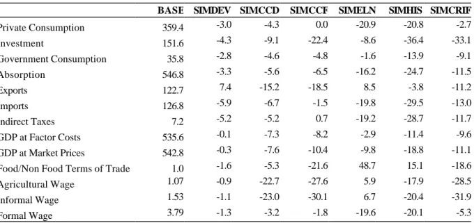
The base CGE scenario seeks to reproduce the evolution of the Indonesian economy
between 1997 and 1998 in terms of changes in employment, wages, and macroeconomic
aggregates. The most important external shocks during that period are the financial crisis and the
extended El Nino drought. The financial crisis is simulated through a combination of different shocks. First, we assume the Indonesia currency suffered a real depreciation of 10% (SIMDEV). Second, all
sectors experienced a “credit crunch”, simulated through a cut in the two types of working capital
used by activities. One experiment examines the impact of a cut of 15% in the availability of domestic
working capital (SIMCCD), while another examines the impact of a 25% cut in the availability of foreign credit crunch (SIMCCF). The drought is simulated through a 10% decrease of total factor
productivity in the agricultural sector, the livestock sector, and the forestry sector, and the food
processing sector, as well as through a 5% increase in the stocks of food commodities and a two
fold increase in the cost of marketing of food (SIMELN). The last components of the shock are supposed to reproduce the hoarding of food products, particularly of rice, that was observed during
the financial crisis, and contributed to the increase in the relative price of food. Each shock is
simulated independently and then combined in the next simulation (SIMHIS). The last simulation
(SIMCRIF) combines the three shocks related to the financial crisis, leaving aside the El Nino drought.
The changes in employment wage and self-employment income derived from the CGE model are taken down to the microsimulation level in order to decompose the contribution of different
shocks and isolate the impact of the financial crisis on poverty. Table 5 shows the contribution of the
different elements of the shock to the total negative real GDP shock. The combination of the different
shocks show that they are not additive. This result can be explained partly because of the specification of the two credit crunch shocks: whenever one type of working capital becomes
binding, physical capital becomes redundant. Although the credit crunch shocks are important driving
forces explaining the collapse of GDP, the contribution of the El Nino drought to total GDP decrease
is not negligible. The drought is also the main driving force explaining the increase in the relative price of food with respect to non-food commodities.
In terms of the impact of poverty and income distribution, microsimulation results from Table
6 show that the head count ratio increased by 76.0% for the historical simulation (SIMHIS). That
increase appears to be fuelled by the decrease in income per capita as well as by an important
increase in inequality indicators. Again, the contribution of the drought appears very important, since the financial shock alone (SIMCRIF) would probably have led to a smaller increase in poverty
indicators. From the perspective of the methodological contribution, the RHG approach produces
results in terms of head count ratio (P0) that are relatively close to the ones produced using the
FULL approach, but since it does not capture the increase in inequality, it systematically underestimates the increase. This bias is even stronger on higher order indicators of poverty: for the
historical experiment, the RHG approach underestimates changes in poverty gap and severity (P1
and P2) by 27 and 39%. This result is not surprising given that these indexes are more sensitive that
the headcount to changes income distribution.
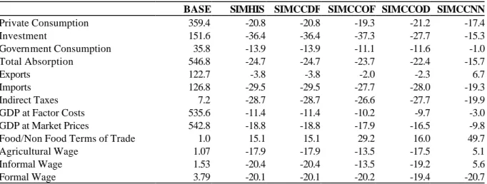
The second set of experiments examines the impact of the adjustment process with no credit
crunch shocks. Experiment SIMCCDF reproduces exactly the historical shock but with a different
specification of the foreign savings closure. While in the historical simulation, foreign savings are
flexible and the exchange rate is fixed to a new level to capture the devaluation shock, the same shock is obtained in SIMCCDF by fixing the foreign savings to the post crisis level and flexing the
exchange rate. Experiment SIMCOF uses the same specification of the foreign savings closure but
without the domestic credit crunch shock. The main difference is the evolution of the relative price of
food: without the domestic crunch shock, the food price increase is double the one obtained in the previous simulation. By contrast, the following simulation (SIMCCOD) does not show a significantly
different impact on macro aggregates, although the GDP decrease is less strong than in the historical
shock. The real difference appears with the last simulation of this set (SIMCCNN) were the
adjustment of the trade balance is imposed with no credit crunch shocks. The impact on GDP is much smaller than in the historical simulation, average agricultural and informal wages go up by 5%.
That income effect translates into a much higher increase in the relative price of food.
Results from the microsimulation module (Table 9) show that without the foreign credit
simulation, due to the higher increase in the relative price of food. The even higher increase in the last
simulation is compensated by the increase in real average wages for agricultural and informal sectors,
leading to a much smaller increase in poverty indicators. Results obtained using the RHG approach,
show that the “within-group-fixed-income-distribution” assumption leads, in the context of the shock examined, to an underestimation of the increase in inequality, thus leading to lower estimates of the
increase in poverty. The approach nevertheless captures some of the effects described above.
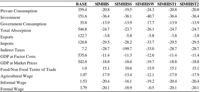
The last set of experiments examines different social policy packages designed to protect the
poor. This set of simulation is described in Table 10. These experiments are designed so that their
total cost is the same and equal to 3% of total household income and 28% of the government
budget. The evolution of macro aggregates in Table 11 suggests that the general equilibrium effects of these programs are relatively small. The CGE framework appears nevertheless useful to design
programs that are equivalent in terms of costs, since these are influenced by general equilibrium
effects. It appears that the total amount spent allows putting in place a 5% subsidy on food prices, or
increasing 2.5 fold transfers to households, or is equivalent to hiring almost 10% of the unskilled labor force at a wage equal to 90% of the market wage for this type of labor. The bottom lines of
Table 11 show, that the food price subsidy achieves partly its goal by lowering by 30% the increase
in the relative price of food, while the public work program contributes to a lesser decrease in the
average formal wage. The macro impacts of the last two simulations are negligible since the increase in the transfer has no effect on factor markets or the relative price of food. Because of the closure
chosen, increasing transfers amounts to redistributing income among households and has no real
effect on the economy.
In terms of poverty and inequality, these programs appear relatively different (Table 12). The
food subsidy program leads to a much lesser increase in the poverty rate, gap and severity compared
to the historical simulation. The public work program achieves an even lesser increase in the poverty indicators. But the most efficient policy package to reduce poverty appears to be the household
transfers. The difference between the two transfer programs lies on the targeting. Both program
pre-crisis poor households (the transfer is nevertheless proportional to the household) while the
second program has perfect information on pre-crisis income levels and thus gives to each household
an amount per capita proportional to the difference between each households per capita income and
the per capita poverty line. Results show that the first program achieves a bigger decrease in the poverty indicators. This can be explained by the fact that there appears to be no strong correlation
between the pre-crisis income level and the post crisis income level. Finally, results obtained using
the RHG approach appear significantly biased for the last two simulations, showing that RHG
framework cannot be used to analyze the impact of targeted programs.
5. Conclusion
Compared to standard CGE or before-after analysis, the framework developed in this paper
allows us to decompose the effects of the financial crisis as well as to compare the impact of
introducing alternative social policy packages, without resorting to the representative household
assumption. It has been shown that this assumption leads to (1) biased results in most experiments, and to (2) incorrect results in the case of targeted policies. In the context of the shocks examined
here, the bias is a systematic underestimation of the impact on inequality, leading to an
underestimation of the impact on poverty.
The first set of experiments shows that the El Nino drought was responsible for at least half
of the increase in poverty indicators during the period, while the credit crunch shock contributed to
the other half. Results from the second set of experiment show that a better management of the credit crunch shocks with the same level of adjustment of the economy would have resulted in a lesser
increase in poverty. Finally, the last experiments show that among three types of social policy
packages, household transfers programs are the most efficient to reduce poverty but that targeting on
References
Alatas, V. and F. Bourguignon. 2000. “The evolution of the distribution of income during Indonesian fast growth: 1980-1996”. Mimeo. Princeton University.
Azis, I. and E. Thorbecke. 2001.
Booth, A. 1998. “The Impact of the Crisis on Poverty and Equity”. ASEAN Economic Bulletin. Vol. 15, No. 3.
Bourguignon, F., F. Ferreira, and N. Lustig (1998), The microeconomics of income distribution dynamics, a research proposal, The Interamerican Bank and the World Bank, Washington Bourguignon F., M. Fournier, and M. Gurgand (2001), Fast Development with a Stable Income
Distribution:Taiwan, 1979-1994, Review of Income and Wealth (June).
Central Bureau of Statistics (CBS). 1998. “Perhitungan Jumlah Penduduk Miskin dengan GNP Per Kapita Riil”. Mimeo. Jakarta.
Frankenberg E., D. Thomas, and K. Beegle. 1999. “The Real Cost of Indonesia’s Economic Crisis: Preliminary Findings from the Indonesia Familiy Life Surveys. International Labour Organization (ILO). 1998. Employment Challenges for the Indonesian Economic Crisis. Jakarta: ILO and United Nations Development Program.
Islam, R. 1998. “Indonesia: Economic Crisis, Adjustment, Employment and Poverty”. Issues in Development Discussion Paper No. 23. Geneva: ILO.
Levinsohn, J., S. Berry, and J. Friedman. 1999. “Impacts of the Indonesian Crisis: Price Changes and the Poor”. NBER Working Paper No. 7194. Cambridge, MA: NBER.
Manning, C. 2000. “Labour Market Adjustment to Indonesia’s Economic Crisis: Context, Trends and Implications”. Bulletin of Indonesian Economic Studies Vol. 36, No. 1.
Plumb, M. (2001), Empirical tax modeling: an applied general equilibrium model for the UK incorporating micro-unit household data and imperfect competition, Dphil Thesis, Nuffield College, University of Oxford.
Pradhan, M., A. Suryahadi, S. Sumarto, and L. Pritchett. 2000. “Measurements of Poverty in Indonesia: 1996, 1999, and Beyond”. Research Working Paper. SMERU.
Suryahadi, A., S. Sumarto, Y. Suharso, and L. Pritchett. 2000. “The Evolution of Poverty during the Crisis in Indonesia, 1996-99”. Research Working Paper. SMERU.
World Bank. 1998. Indonesia in Crisis: A Macroeconomic Update. Washington, D.C.: World Bank.
Table 1: Indices of Poverty in Indonesia, 1997-1998
All Urban Rural
1996 1999% change 1996 1999 % change 1996 1999% change Head-Count Index (P0) 9.75 16.27 66.8% 3.82 9.63 152.3% 13.10 20.56 56.9% Poverty Gap Index (P1) 1.55 2.79 80.2% 0.53 1.51 183.0% 2.12 3.61 70.5% Poverty Severity Index (P2) 0.39 0.75 91.9% 0.12 0.37 201.6% 0.54 0.99 83.6% Source: Suryahadi et al. (2000) based on SUSENAS surveys 1996 and 1999.
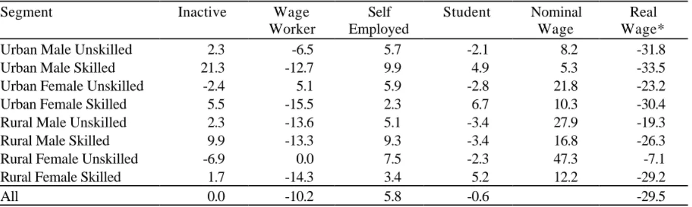
Table 2: Evolution of occupational choices and wages by segment 1997-1998.
Segment Inactive Wage
Worker Self Employed Student Nominal Wage Real Wage*
Urban Male Unskilled 2.3 -6.5 5.7 -2.1 8.2 -31.8
Urban Male Skilled 21.3 -12.7 9.9 4.9 5.3 -33.5
Urban Female Unskilled -2.4 5.1 5.9 -2.8 21.8 -23.2
Urban Female Skilled 5.5 -15.5 2.3 6.7 10.3 -30.4
Rural Male Unskilled 2.3 -13.6 5.1 -3.4 27.9 -19.3
Rural Male Skilled 9.9 -13.3 9.3 -3.4 16.8 -26.3
Rural Female Unskilled -6.9 0.0 7.5 -2.3 47.3 -7.1
Rural Female Skilled 1.7 -14.3 3.4 5.2 12.2 -29.2
All 0.0 -10.2 5.8 -0.6 -29.5
Source: SAKERNAS 1997, 1998. *deflated by CPI base year 1996 = 100.
Table 3: Historical Simulation Results
All Urban Rural
Base % change Base % change Base % change Per Capita Income 121.1 -21.8 170.9 -25.9 90.6 -17.1
Theil Index 49.3 9.2 53.9 16.9 33.1 12.8
Gini Index 45.6 3.2 47.5 7.8 38.7 4.5
Head-Count Index (P0) 10.7 97.8 4.7 204.4 14.3 76.3
Poverty Gap Index (P1) 2.6 136.0 1.2 251.1 3.4 111.0 Poverty Severity Index (P2) 1.0 160.9 0.5 295.5 1.4 131.6 Source: Results from microsimulation module using historical changes in prices, wages and occupational choices by segment (see Table 2). Self employment income is assumed to be cut by 20 and 15% for agricultural activities in the urban and rural sectors respectively, and by 25% and 20% for non agricultural activities.
Table 4: CGE Simulations - Decomposing the historical shock
Simulation Name Description SIMDEV Real devaluation SIMCCD Domestic Credit Crunch SIMCCF Foreign Credit Crunch SIMELN El Nino Drought
SIMHIS SIMDEV + SIMCCD + SIMCCF + SIMELN SIMCRIF SIMDEV + SIMCCD + SIMCCF
Table 5: Simulation Results: Macro Aggregates (base values and percent change)
BASE SIMDEV SIMCCD SIMCCF SIMELN SIMHIS SIMCRIF
Private Consumption 359.4 -3.0 -4.3 0.0 -20.9 -20.8 -2.7 Investment 151.6 -4.3 -9.1 -22.4 -8.6 -36.4 -33.1 Government Consumption 35.8 -2.8 -4.6 -4.8 -1.6 -13.9 -9.1 Absorption 546.8 -3.3 -5.6 -6.5 -16.2 -24.7 -11.5 Exports 122.7 7.4 -15.2 -18.5 8.5 -3.8 -11.2 Imports 126.8 -5.9 -6.7 -1.5 -19.8 -29.5 -13.0 Indirect Taxes 7.2 -5.2 -5.2 0.7 -19.2 -28.7 -11.7 GDP at Factor Costs 535.6 -0.1 -7.3 -8.2 -2.9 -11.4 -9.6 GDP at Market Prices 542.8 -0.3 -7.6 -10.4 -9.8 -18.8 -11.1 Food/Non Food Terms of Trade 1.0 -1.6 -5.3 -21.6 48.7 15.1 -18.6
Agricultural Wage 1.07 -0.9 -22.7 -27.6 5.9 -17.9 -28.5
Informal Wage 1.53 -1.1 -23.0 -30.1 6.7 -20.4 -31.9
Formal Wage 3.79 -1.3 -3.2 -1.8 -19.6 -20.1 -5.3
Table 6: Simulation Results: PCI, inequality, and poverty indicators (base values and % changes)
FULL BASE SIMDEV SIMCCD SIMCCF SIMELN SIMHIS SIMCRIF
Per Capita Income 121.1 -0.8 -8.8 -9.9 -7.5 -16.1 -12.1
Theil Index 49.3 0.4 4.5 -4.0 15.6 8.8 -0.9
Gini Index 45.6 0.2 2.7 -1.5 6.2 3.4 -0.1
Head-Count Index (P0) 10.7 3.2 49.6 24.5 53.1 76.0 41.9
Poverty Gap Index (P1) 2.6 5.9 59.8 30.9 76.4 100.1 52.7
Poverty Severity Index (P2) 1.0 8.2 61.8 30.3 95.0 117.0 56.6
RHG BASE SIMDEV SIMCCD SIMCCF SIMELN SIMHIS SIMCRIF
Per Capita Income 121.1 -0.8 -8.8 -10.1 -7.7 -16.0 -12.2
Theil Index 49.3 0.1 2.8 -2.0 2.7 0.9 -0.8
Gini Index 45.6 0.1 1.7 -1.0 1.4 0.5 -0.4
Head-Count Index (P0) 10.7 3.0 41.8 30.2 34.6 63.0 41.1
Poverty Gap Index (P1) 2.6 2.8 48.1 33.0 38.5 73.5 46.8
Table 7: CGE Simulations - Macroeconomic Counterfactuals
Simulation Name Description
SIMHIS Historical experiment
SIMCCDF Historical experiment fixing adjustment of the trade balance SIMCCOF Historical experiment with no domestic credit crunch SIMCCOD Historical experiment with no foreign credit crunch SIMCCNN Historical experiment with no credit crunch
Table 8: Simulation Results: Macro Aggregates (base values and percent change)
BASE SIMHIS SIMCCDF SIMCCOF SIMCCOD SIMCCNN
Private Consumption 359.4 -20.8 -20.8 -19.3 -21.2 -17.4 Investment 151.6 -36.4 -36.4 -37.3 -27.7 -15.3 Government Consumption 35.8 -13.9 -13.9 -11.1 -11.6 -1.0 Total Absorption 546.8 -24.7 -24.7 -23.7 -22.4 -15.7 Exports 122.7 -3.8 -3.8 -2.0 -2.3 6.7 Imports 126.8 -29.5 -29.5 -27.7 -28.0 -19.3 Indirect Taxes 7.2 -28.7 -28.7 -26.6 -27.7 -19.9 GDP at Factor Costs 535.6 -11.4 -11.4 -10.2 -9.7 -3.0 GDP at Market Prices 542.8 -18.8 -18.8 -17.9 -16.5 -9.8
Food/Non Food Terms of Trade 1.0 15.1 15.1 29.2 16.0 49.7
Agricultural Wage 1.07 -17.9 -17.9 -13.5 -17.5 5.1
Informal Wage 1.53 -20.4 -20.4 -13.5 -19.2 5.6
Formal Wage 3.79 -20.1 -20.1 -20.2 -19.4 -20.7
Table 9: Simulation Results: PCI, inequality, and poverty indicators (base values and % changes)
FULL BASE SIMHIS SIMCCDF SIMCCOF SIMCCOD SIMCCNN
Per Capita Income 121.1 -16.1 -16.1 -15.7 -14.2 -8.3
Theil Index 49.3 8.8 8.8 8.3 14.6 16.4
Gini Index 45.6 3.4 3.4 3.2 6.1 6.7
Head-Count Index (P0) 10.7 76.0 76.0 72.4 84.0 58.2
Poverty Gap Index (P1) 2.6 100.1 100.1 96.9 114.7 86.0
Poverty Severity Index (P2) 1.0 117.0 117.0 114.1 134.7 107.1
RHG BASE SIMHIS SIMCCDF SIMCCOF SIMCCOD SIMCCNN
Per Capita Income 121.1 -16.0 -16.0 -15.7 -14.3 -8.5
Theil Index 49.3 0.9 0.9 0.6 3.7 2.7
Gini Index 45.6 0.5 0.5 0.4 2.1 1.4
Head-Count Index (P0) 10.7 63.0 63.0 62.0 66.5 37.6
Poverty Gap Index (P1) 2.6 73.5 73.5 70.3 77.8 42.3
Table 10: CGE Simulations - Social Policy Packages
Simulation Name Description
SIMHIS Historical experiment (see Table 4) SIMHISS SIMHIS + food price subsidy
SIMHISW SIMHIS + public work program for all unskilled workers SIMHIST1 SIMHIS + imperfectly targeted household transfer SIMHIST2 SIMHIS + perfectly targeted household transfer
Table 11: Simulation Results: Macro Aggregates (base values and % changes)
BASE SIMHIS SIMHISS SIMHISW SIMHIST1 SIMHIST2
Private Consumption 359.4 -20.8 -19.5 -24.3 -20.8 -20.8 Investment 151.6 -36.4 -36.1 -40.7 -36.4 -36.4 Government Consumption 35.8 -13.9 -13.9 17.7 -13.9 -13.9 Total Absorption 546.8 -24.7 -23.7 -26.1 -24.7 -24.7 Exports 122.7 -3.8 -5.8 -5.8 -3.8 -3.8 Imports 126.8 -29.5 -28.2 -33.7 -29.5 -29.5 Indirect Taxes 7.2 -28.7 -199.7 -33.0 -28.7 -28.7 GDP at Factor Costs 535.6 -11.4 -11.3 -12.6 -11.4 -11.4 GDP at Market Prices 542.8 -18.8 -18.6 -19.7 -18.8 -18.8
Food/Non Food Terms of Trade 1.0 15.1 10.6 15.9 15.1 15.1
Agricultural Wage 1.07 -17.9 -13.4 -12.1 -17.9 -17.9
Informal Wage 1.53 -20.4 -16.1 -19.2 -20.4 -20.4
Formal Wage 3.79 -20.1 -18.9 -0.5 -20.1 -20.1
Table 12: Simulation Results: PCI, inequality, and poverty indicators (base values and % changes)
FULL BASE SIMHIS SIMHISS SIMHISW SIMHIST1 SIMHIST2
Per Capita Income 121.1 -16.1 -13.7 -15.3 -13.0 -13.0
Theil Index 49.3 8.8 6.3 2.3 -2.1 -1.3
Gini Index 45.6 3.4 2.4 0.3 -5.0 -3.8
Head-Count Index (P0) 10.7 76.0 57.8 54.9 -23.0 -7.5
Poverty Gap Index (P1) 2.6 100.1 78.9 72.0 -50.8 -43.4
Poverty Severity Index (P2) 1.0 117.0 94.8 78.2 -50.5 -46.5
RHG BASE SIMHIS SIMHISS SIMHISW SIMHIST1 SIMHIST2
Per Capita Income 121.1 -16.0 -13.6 -15.2 -12.9 -12.9
Theil Index 49.3 0.9 -0.2 -2.7 -2.8 -2.8
Gini Index 45.6 0.5 -0.2 -1.5 -1.7 -1.6
Head-Count Index (P0) 10.7 63.0 47.7 45.3 34.2 34.3
Poverty Gap Index (P1) 2.6 73.5 54.4 51.8 37.9 37.9