Modeling of the flood regimes in coupled stream-aquifer systems

HAL Id: pastel-00003360

https://pastel.archives-ouvertes.fr/pastel-00003360

Submitted on 21 Feb 2008

HAL is a multi-disciplinary open access archive for the deposit and dissemination of sci-entific research documents, whether they are pub-lished or not. The documents may come from teaching and research institutions in France or

L’archive ouverte pluridisciplinaire HAL, est destinée au dépôt et à la diffusion de documents scientifiques de niveau recherche, publiés ou non, émanant des établissements d’enseignement et de recherche français ou étrangers, des laboratoires

Modeling of the flood regimes in coupled stream-aquifer

systems

Serdar Korkmaz

To cite this version:

Serdar Korkmaz. Modeling of the flood regimes in coupled stream-aquifer systems. Sciences of the Universe [physics]. École Nationale Supérieure des Mines de Paris, 2007. English. �NNT : 2007ENMP1495�. �pastel-00003360�

MODELING OF THE FLOOD REGIMES IN COUPLED STREAM-AQUIFER SYSTEMS

A THESIS SUBMITTED TO

ECOLE DOCTORALE GEOSCIENCES ET RESSOURCES NATURELLES PARIS OF

ECOLE DES MINES DE PARIS AND

THE GRADUATE SCHOOL OF NATURAL AND APPLIED SCIENCES OF

MIDDLE EAST TECHNICAL UNIVERSITY

BY

SERDAR KORKMAZ

IN PARTIAL FULFILLMENT OF THE REQUIREMENTS FOR THE DEGREE OF DOCTEUR

IN

HYDROLOGIE ET HYDROGEOLOGIE QUANTITATIVES AND

THE DEGREE OF DOCTOR OF PHILOSOPHY IN

CIVIL ENGINEERING

Approval of the thesis:

MODELING OF THE FLOOD REGIMES IN COUPLED STREAM-AQUIFER SYSTEMS

submitted by SERDAR KORKMAZ in partial fulfillment of the requirements for the degree of Docteur in Hydrologie et Hydrogéologie Quantitatives, Ecole des Mines de Paris and Doctor of Philosophy in Civil Engineering Department, Middle East Technical University by,

Prof. Dr. Canan Özgen _____________________ Dean, Graduate School of Natural and Applied Sciences

Prof. Dr. Güney Özcebe _____________________

Head of Department, Civil Engineering

Prof. Dr. Halil Önder _____________________ Supervisor, Civil Engineering Dept., METU

Dr. Emmanuel Ledoux _____________________

Supervisor, Centre de Géosciences, ENSMP

Examining Committee Members:

Prof. Dr.Pierre Ribstein (France) _____________________ Université Paris 6

Prof. Dr. Halil Önder _____________________

Civil Engineering Dept., METU

Dr. Emmanuel Ledoux (France) _____________________ Centre de Géosciences, Ecole des Mines de Paris

Prof. Dr. Turgut Tokdemir _____________________ Engineering Sciences Dept., METU

Assoc. Prof. Dr. İsmail Aydın _____________________ Civil Engineering Dept., METU

Dr. Eric Martin (France) _____________________ Météo-France

Dr. Thierry Pointet (France) _____________________ Bureau de Recherches Géologiques et Minières

I hereby declare that all information in this document has been obtained and

presented in accordance with academic rules and ethical conduct. I also declare that, as required by these rules and conduct, I have fully cited and referenced all material and results that are not original to this work.

Name, Last name : Serdar Korkmaz

ABSTRACT

M

ODELING OF THE

F

LOOD

R

EGIMES IN

C

OUPLED

S

TREAM

-A

QUIFER

S

YSTEMS

Korkmaz, Serdar

Ph.D., Department of Civil Engineering (METU) Ph.D., Centre de Géosciences (ENSMP)

Supervisor : Prof. Dr. Halil Önder Supervisor : Dr. Emmanuel Ledoux

December 2007, 166 pages

In this study, hydrogeological modeling of the Somme river basin situated in the north of France was made with special emphasis on the stream-aquifer interaction. The coupled model developed at Ecole des Mines de Paris was used. Geographic Information Systems (GIS) tools were incorporated during all the stages of modeling process for both preparation of input data and visualization of the results of simulations. Initially, the process began with Digital Elevation Model (DEM) analysis. Afterwards, the surface and aquifer grids were generated by using nested grid generators and refinement was made on the stream network and subcatchment boundaries in order to increase the accuracy of numerical solution. In order to run the surface model, meteorological forcing, land use and soil type data were acquired. Surface model was used to partition the precipitation into evapotranspiration, infiltration and surface runoff components. A steady-state piezometric head distribution was computed by the groundwater model to serve as an initial condition to the coupled model. The flow in the unsaturated zone was simulated by using Nash cascade model. The unsteady groundwater and surface flow simulations were performed by taking into consideration the stream-aquifer interaction on a daily time step. The calibration and validation were realized by using the streamflow and piezometric head measurements distributed around the basin. The strong groundwater influence on the

hydrology of the basin is well represented by the model. Comparisons of predicted flooded areas in year 2001 were made with other models and a satellite derived image. In the end, several sensitivity analyses were performed for several parameters concerning the groundwater flow.

Keywords: hydrology, hydrogeology, coupled model, flood, stream-aquifer interaction, GIS, DEM, sensitivity analysis.

RESUME

M

ODÉLISATION DES

R

ÉGIMES DE

C

RUE DES

S

YSTÈMES

C

OUPLÉS

A

QUIFÈRES

-R

IVIÈRES

Korkmaz, Serdar

Ph.D., Department of Civil Engineering (METU) Ph.D., Centre de Géosciences (ENSMP)

Directeur de thèse: Prof. Dr. Halil Önder Directeur de thèse: Dr. Emmanuel Ledoux

Décembre 2007, 166 pages

Dans ce travail, une modélisation hydrogéologique du bassin-versant de la Somme dans le nord de la France a été menée avec une attention particulière sur l’interaction rivière-aquifère. Le modèle couplé développé à l’Ecole des Mines de Paris a été utilisé. Un Système d’Information Géographique a été incorporé à toutes les étapes du processus de modélisation pour la préparation des données d’entrée et la visualisation des résultats des simulations. Le processus commence tout d’abord par l’analyse du Modèle Numérique de Terrain (MNT). Ensuite, les maillages de surface et de l’aquifère ont été créés avec un mailleur gigogne. Une discrétisation plus fine a été effectuée sur le réseau des rivières et les limites des sous-bassins dans le but d’augmenter la précision de la solution numérique. Pour faire tourner le modèle de surface, des données météorologiques, d’occupation du sol et de type de sol ont été acquises. Le modèle de surface permet de répartir les précipitations en évapotranspiration, infiltration et ruissellement de surface. Des niveaux piézométriques en régime permanent sont calculés par le modèle de nappe et constituent les conditions initiales du modèle couplé. L’écoulement dans la zone non saturée a été simulé par un modèle utilisant la cascade de Nash. Les simulations d’écoulement transitoire souterrain et de surface ont été réalisées en prenant en compte les interactions nappe-rivière sur un pas de temps journalier. La calibration et la

validation des résultats ont été faites en utilisant les mesures des débits et des niveaux piézométriques dans le bassin. La forte influence de la nappe sur le régime hydrologique du bassin est bien représentée par le modèle. Des comparaisons de prédiction des zones inondées en 2001 ont été effectuées avec d’autres modèles et une image satellitaire. Enfin, des analyses de sensibilité pour plusieurs paramètres d’écoulement souterrain ont été réalisées.

Mots-clés: hydrologie, hydrogéologie, modèle couplé, inondation, interaction nappe-rivière, SIG, MNT, analyse de sensibilité.

ÖZ

B

İRLEŞİK

N

EHİR

-A

KİFER

S

İSTEMLERİNDE

T

AŞKIN

R

EJİMLERİNİN

M

ODELLENMESİ

Korkmaz, Serdar

Doktora, İnşaat Mühendisliği Bölümü (ODTÜ) Doktora, Centre de Géosciences (ENSMP) Tez Yöneticisi : Prof. Dr. Halil Önder Tez Yöneticisi : Dr. Emmanuel Ledoux

Aralık 2007, 166 sayfa

Bu çalışmada Fransa’nın kuzeyinde yer alan Somme nehir havzasının hidrojeolojik modeli nehir-akifer etkileşimi göz önünde bulundurularak yapılmıştır. Bunun için Ecole des Mines de Paris’te geliştirilen birleşik model kullanılmıştır. Coğrafi Bilgi Sistemleri (CBS) araçları modellemenin bütün aşamalarında girdi verilerinin hazırlanması ve simülasyon sonuçlarının görsellenmesi amacıyla kullanılmıştır. İlk aşamada, Sayısal Yükseklik Modeli (SYM) analizi yapılmış ve havza ile ilgili alansal bilgi çıkartılmıştır. Daha sonra yüzey ve akifer için çözüm ağları oluşturulmuş ve nehirler ile alt havza sınırlarında sayısal çözümün kesinliğini artırmak amacıyla sıklaştırma yapılmıştır. Yüzey modelini kullanabilmek için meteorolojik veriler, arazi kullanımı ve toprak çeşidiyle ilgili veriler elde edilmiştir. Yüzey modeli düşen yağışın buharlaşma, sızma ve yüzey akımı olarak bölümlenmesinde kullanılmıştır. Yeraltı suyu modeli ile birleşik modele başlangıç koşulu oluşturması için sabit bir yeraltı suyu seviyesi hesaplanmıştır. Doymamış bölgedeki akım ise Nash çağlayan modeli ile hesaplanmıştır. Değişken yeraltı ve yüzey suyu akımlarının hesapları günlük zaman dilimleriyle ve de nehir-akifer etkileşimi hesaba katılarak yapılmıştır. Modelin kalibrasyonu ve doğrulanması havza üzerinde bulunan debi ve yeraltı suyu seviyesi ölçümleri ile gerçekleştirilmiştir. Yeraltı suyunun havzanın hidrolojik rejimi üzerindeki güçlü etkisi model tarafından başarıyla temsil edilmiştir.

Diğer modellerle debi ve 2001 yılı taşkın alanları karşılaştırmaları yapılmıştır. Son olarak da yeraltı suyu akımını etkileyen parametrelerle ilgili ilerde veri toplamayı yönlendirmesi amacıyla bir hassasiyet analizi sunulmuştur.

Anahtar Kelimeler: hidroloji, hidrojeoloji, birleşik model, taşkın, nehir-akifer etkileşimi, CBS, SYM, hassasiyet analizi.

ACKNOWLEDGEMENTS

I wish to express my deepest gratitude to my supervisors Prof. Dr. Halil Önder and Dr. Emmanuel Ledoux for their guidance, advice, criticism, encouragements and insight throughout the research.

I also wish to thank Zouheir Hamrouni and the French Embassy staff in Turkey for their help in establishing this Joint PhD program and for the scholarship provided by the French Government during 15 months of my study.

I would like to thank Florence Habets from UMR Sisyphe at Ecole des Mines de Paris, who was responsible of a scientific program on the Somme river basin funded by the Centre National de la Recherche Scientifique (CNRS). Her constant and patient help providing advices all along this study was essential. I would also like to thank the members of the scientific committee of the project who gave me the opportunity of fruitful discussions. My acknowledgments are especially expressed to Dominique Thiéry from BRGM who provided quantity of data about the Somme aquifer system.

From Ecole des Mines, my thanks go to Nicolas Flipo, Pascal Viennot, André Levassor, Christelle Martin, Drissa Diarrassouba, Mounir Salim and all of the professors at Centre de Géosciences for sharing their lunchtimes, giving suggestions, and most of all, for their friendly attitude.

From Middle East Technical University, I would like to thank Mehmet Ata Bodur, Celal Soyarslan and Prof. Dr. Eyüp Özveren for sharing lunchtimes, making funny chats and keeping in touch while I was away.

I would like to acknowledge the assistance provided by the administrative staff of both institutes; in particular, my thanks go to Dominique Vassiliadis, Cahide Gökdemir and Sebay Durul.

I am very grateful to Serdar Ekinci, Hasan Sevinç, Selim Tezcan and Ahmet Düzce for their everlasting friendship and invaluable support during every moment of this long journey.

Finally, I would like to express my eternal gratitude to my parents Günay and Mümtaz, and to my brother Kerem. This PhD thesis would never have become reality without you.

SUMMARY OF THESIS IN FRENCH

Revue bibliographique :

Les interactions entre les eaux superficielles et les eaux souterraines ont fait l’objet d’une attention particulière de la part de nombreux chercheurs. Le phénomène d’interaction nappe-rivière est en effet important pour étudier les événements dangereux de crue et pour optimiser l’exploitation des ressources en eaux de surface et souterraines ; il a aussi des implications majeures sur le plan écologique (Hantush et al. 2002). Selon Sophocleous (2002), la nappe et les eaux de surface ne sont pas les composants isolés d’un système hydrologique, mais interagissent dans une variété de contextes physiographiques et climatiques. Donc, le développement de l’un des aspects concerne habituellement l’autre.

Selon leur position relative dans l’espace, Toth (1963) définit trois types différents de systèmes d’écoulement : local, intermédiaire et régional, qui s’expriment de manière emboitée sur un bassin versant. Dans un système d’écoulement local, l’eau s’écoule vers un exutoire proche comme un étang ou une rivière. Dans un système d’écoulement régional, elle voyage sur une distance plus grande jusqu’aux rivières majeures, aux grands lacs ou aux océans. Le système d’écoulement intermédiaire concerne un domaine situé entre un affluent et un exutoire, mais, contrairement à un système d’écoulement régional, il ne contient ni la tête, ni l’aval du bassin.

La vidange d’une nappe n’est pas seulement localisée le long d’un cours d’eau mais elle se développe aussi à travers la zone de décharge en aval d’une ligne séparant les sous-bassins versants. Il en résulte que, si l’on utilise le débit de base comme indicateur de la recharge moyenne d’un domaine hydrologique, une erreur important peut être introduite, car le débit de base peut ne représenter qu’une petite partie de la décharge totale provenant de ce domaine (Sophocleous 2002).

Larkin et Sharp (1992) classent les systèmes nappe-rivière suivant trois catégories (1) les systèmes dominés par l’inferoflux (le flux de la nappe s’écoule parallèlement à la rivière et dans la même direction qu’elle) ; (2) les systèmes dominés par le débit de base (le flux

de la nappe s’écoule perpendiculairement à la rivière, dans un sens ou dans l’autre selon que la rivière draine ou alimente) ; (3) les systèmes composites ; le mode d’écoulement dominant peut être déduit des données géomorphologiques tels que la pente du cours d’eau, la sinuosité de la rivière, le degré d’incision au sein des alluvions, le rapport largeur sur profondeur de chenal et la nature des dépôts fluviatiles.

Sophocleous (2002) définit le débit de base comme l’eau qui parvient à une rivière sous l’effet d’une alimentation persistante, lentement variable, et qui soutient l’écoulement de la rivière entre les événements de crue. L’écoulement souterrain peut cependant aussi alimenter les rivières assez rapidement pour contribuer à la génération d’événements de forts régimes hydrodynamiques.

Certains chercheurs ont souligné l’influence du domaine souterrain sur les bassins hydrologiques. Par exemple, Beven (2000) indique que l’un des problèmes intervenant dans la compréhension complète des systèmes hydrologiques est que, lorsque la majorité de l’écoulement est de nature souterraine, notre capacité de mesurer et évaluer les processus d’écoulement souterrain est limitée.

Les considérations qui précèdent illustrent l’intérêt, sinon la nécessité, d’être capable de modéliser conjointement les écoulements de surface et les écoulements souterrains pour de nombreux cas de systèmes hydrologiques.

Objectifs :

Le bassin versant de la Somme dans le nord de la France a été concerné par une très forte crue pendant l’année 2001 durant laquelle les eaux ont atteint des cotes exceptionnelles et causé un dommage majeur à l’environnement. Cet événement a souligné la contribution des aquifères à l’hydrologie du bassin. Selon une estimation du BRGM (Bureau de Recherches Géologiques et Minières), près de 75% du volume de crue a été provoqué par l’exfiltration de la nappe à la surface du sol et par l’échange direct entre la nappe et la rivière. Le même événement a, par la suite, joué un rôle important dans le soutien des débits et il a atténué les conséquences de saisons sèches ultérieures telles que rencontrées au cours du printemps et de l’été 2003. En conséquence, dans ce travail de recherche, une modélisation hydrogéologique complète du bassin versant de la Somme a été menée avec une attention particulière portant sur l’interaction rivière-aquifère.

Résumé de la recherche :

Dans ce travail, un modèle hydrologique couplée du bassin versant de la Somme dans le nord de la France a été construit avec une attention particulière sur l’interaction rivière-aquifère. La modélisation a été basée sur le modèle couplé (MODCOU) développé à l’Ecole des Mines de Paris. Les outils SIG ont été utilisés pendant toutes les étapes de modélisation pour la préparation des données d’entrée puis la visualisation et l’exploitation des résultats de simulation.

Le processus de construction du modèle commence tout d’abord par l’extraction d’informations spatiales sur le bassin en s’appuyant sur l’analyse du Modèle Numérique de Terrain (MNT). Basée sur une image « raster » de la topographie avec une taille de pixel de 125 m, cette analyse a consisté à déterminer les directions de drainage, les surfaces drainées, à construire le réseau hydrographique, puis à partitionner le bassin en sous-bassins versants. Ces analyses ont été faites au moyen du programme HYDRODEM mis à disposition dans le cadre d’un partenariat avec le Cemagref de Lyon.

Après l’acquisition des données spatiales, une discrétisation du domaine de surface en mailles carrées emboitées a été créé par le program SIGMOD. Une discrétisation plus fine a été employée sur le réseau des rivières et les limites des sous-bassins dans le but d’augmenter la précision de la solution numérique dans ces secteurs importants sur le plan hydrologique. Le maillage le plus approprié a été obtenu par tâtonnement. Plusieurs maillages ont ainsi été créés selon les réseaux de rivière retenus pour des seuils différents de la surface drainée par le réseau hydrographiques. Les petits sous-bassins versants ont été regroupés, lorsque cela était possible, pour éviter les raffinements inutiles. Les limites du domaine ont été étendues jusqu’aux plus proches limites naturelles telles que les rivières principales des bassins voisins, de manière à atteindre des conditions aux limites de piézométrie imposée pour l’aquifère. Cette démarche était nécessaire, car, dans le cas de la Somme, l’aquifère présente une extension régionale qui dépasse les limites du bassin versant superficiel. Ensuite, le maillage de l’aquifère a été créé au moyen du programme SIGSOU exactement sur la même géométrie spatiale que la couche de surface pour permettre la représentation de l’interaction surface-souterrain en chaque point du bassin. La procédure de regroupement des mailles intégrée aux programmes de maillage a été mise en œuvre pour réduire le nombre de mailles du modèle sur les pentes des sous-bassins versants loin des lignes de partage des eaux ; cependant, la discrétisation fine a été conservée au niveau des mailles rivières pour maintenir la précision dans l’interaction

nappe-rivière. Après la création des maillages, 71653 mailles pour la couche de surface et 63226 mailles pour la couche aquifère ont été retenues, les tailles des mailles se répartissant entre 125, 250, 500 et 1000 m.

Le modèle couplé se compose de 4 modules principaux, à savoir, MODSUR, NEWSAM, NONSAT and MODCOU. Pour exécuter le modèle de surface, MODSUR, les forçages météorologiques, les données d’occupation de sol et de type de sol sont requises. Le forçage météorologique (précipitation et évapotranspiration potentielle) a été fourni par Météo-France selon la procédure Safran sur un maillage couvrant la surface de bassin avec des mailles ayant une taille de 8 km, sur la période allant du 1/8/1985 au 31/7/2003 avec un pas de temps journalier. Les données d’occupation de sol proviennent de la base de données CORINE Land Cover et celles portant sur les types de sol de la base de données INRA au 1/1000000. Les données d’occupation de sol et de type de sol ont ensuite été croisées sous l’environnement SIG ArcGIS dans le but de construire les zones de production permettant la spatialisation du bilan hydrique en surface du bassin. Le programme MODSUR utilise une fonction production qui partage la précipitation entre ruissellement, infiltration et évapotranspiration réelle selon ces zones de production. Le programme calcule ensuite le volume de l’eau s’infiltrant sur chaque maille de surface, puis le volume d’eau arrivant dans chaque maille rivière à chaque pas de temps. La mise en œuvre de la fonction production de MODSUR nécessite la définition d’un jeu de paramètres propre à chaque zone de production. Pour identifier les valeurs optimales de ces paramètres une procédure de calibration a été suivie sur la période 1/8/1995-31/7/2003. L’effet de chaque paramètre sur l’hydrogramme de la Somme à Abbeville (5560 km2_{) a été analysé et décrit en détail. En fin de calibration, un contrôle de validité}

du modèle a été fait sur la période 1/8/1985-31/7/1995. Les critères statistiques obtenus à l’issue du calage ont été assez satisfaisants, conduisant par exemple à un coefficient de Nash-Sutcliffe de 0,93 sur la période de calibration, de 0,72 sur celle de validation et de 0,86 pour la période globale.

Le module logiciel intervenant en second lieu est NEWSAM qui simule l’écoulement en aquifère. Dans ce travail, il a été utilisé en régime permanent pour obtenir un niveau piézométrique initial. Pour ce faire, la moyenne des valeurs d’infiltration calculée sur la période de calage de MODSUR a été introduite en entrée du modèle souterrain. Une première estimation des paramètres hydrodynamiques (perméabilité et coefficient d’emmagasinement) a été fournie par le BRGM. En fonction de la disponibilité de ces

données, les perméabilités ont été définies sur 5 zones et transférées sur le maillage grâce au SIG. Comme le modèle utilise la transmissivité pour simuler l’écoulement, cette grandeur a été obtenue à partir des valeurs de perméabilité et de l’épaisseur moyenne de la nappe également fournie par le BRGM.

Les simulations en régime transitoire de l’écoulement de surface et de l’écoulement en nappe ont été effectuées avec le programme MODCOU. Ce programme simule le transfert en rivière et l’écoulement souterrain en tenant compte de l’interaction rivière-nappe. Comme données d’entrée, il est nécessaire de fournir les valeurs journalières de ruissellement en chaque maille rivière (calculées par MODSUR), l’alimentation journalière de la nappe (calculée par NONSAT en sortie de MODSUR), un niveau initial de piézométrie, la transmissivité, le coefficient d’emmagasinement, les prélèvements en nappe et les paramètres caractérisant la relation nappe-rivière (niveau de drainage, coefficient de transfert, débit maximal réinfiltrable), issus de NEWSAM. MODCOU fournit en sortie les débits journaliers aux stations hydrométriques et à l’exutoire du bassin, les chroniques piézométriques journalières en 50 point du domaine et la carte piézométrique de l’aquifère en fin de chaque année. Une calibration élaborée a été faite et chaque étape en a été décrite en détail. Au départ, une première calibration en régime permanent a porté sur les transmissivités en recherchant une correspondance entre la structure des cartes piézométriques simulées et observées. Les résultats ont ensuite été affinés en régime transitoire en réglant le coefficient d’emmagasinement et, si nécessaire, à nouveau la transmissivité pour reproduire au mieux les chroniques piézométriques. Au cours de la démarche de calage, un problème de représentation topographique a été mis en évidence se manifestant sous la forme de maximum ou de minimum locaux dans le MNT, préjudiciables à une bonne simulation des échanges hydriques entre le domaine de surface et le domaine souterrain, les variations parasites de l’altitude causant des irrégularités sur l’exfiltration calculée. Un programme a été écrit en FORTRAN pour appliquer une procédure de lissage au MNT sur l’ensemble de la surface du domaine et plus spécifiquement le long des rivières, pour lesquelles la résolution assez moyenne (125 m) du MNT était notablement insuffisante. Après l’exécution de cette procédure, un réajustement moyen de 0,03 m a été appliqué sur la surface du bassin. Sur chaque branche de rivière, les élévations des mailles ont été ramenées sur la ligne de pente moyenne de façon à rétablir une décroissance continue de l’amont vers l’aval là où cela était nécessaire. Cette correction a apporté une amélioration significative au calcul de l’exfiltration le long de réseau hydrographique. Dans une seconde étape, les valeurs

initiales de coefficient d’emmagasinement et de la transmissivité ont été reprises pour affiner le calage piézométrique local du modèle ; une amélioration nette a été obtenue sur 43 parmi les 50 stations piézométriques disponibles. Les retouches les plus importantes des paramètres du modèle ont eu lieu sur les sous-bassins de l’Avre et de la Selle. La dernière étape de calibration a porté sur le coefficient de tarissement des mailles rivières qui contrôle le transfert de l’eau d’une maille rivière à l’autre et finalement d’un bief à l’autre. Sa calibration a eu une bonne influence sur les hydrogrammes de l’Avre, de la Selle et de l’Hallue, particulièrement, en réduisant les pics qui parasitaient les débits calculés.

La simulation de transfert de l’eau dans la zone non-saturée a été menée au moyen du programme NONSAT. NONSAT calcule l’alimentation de la nappe à partir de l’infiltration à la surface préalablement calculé par MODSUR. Ce programme est en réalité exécuté avant MODCOU ; cependant, comme sa calibration a été faite, dans notre étude, après MODCOU, son emploi est décrit en dernier lieu. L’exécution de NONSAT implique d’identifier la répartition spatiale de deux paramètres, soit, le nombre des réservoirs en cascade représentant la colonne de milieu non-saturé et la constante de temps de vidange caractérisant ces réservoirs. L’épaisseur de la zone non-saturée, obtenue par différence entre la cote au sol et la piézométrie moyenne fournie par le BRGM, a été divisée en couches régulières de 5 m, correspondant chacune à un réservoir de transfert. Au final, chaque maille de surface se voit attribuer, en fonction de sa position dans l’espace un nombre de réservoirs et une constante de temps, paramètres qui resteront invariants au cours de la simulation. La calibration de la constante de temps a été menée en deux étapes ; une première valeur de 5 jours a donné les meilleurs résultats globaux sur l’ensemble du domaine ; une calibration plus détaillée a été ensuite effectuée en cherchant à différentier les sous-bassins correspondant à des stations hydrométriques. Cette seconde calibration a amélioré tous les hydrogrammes, particulièrement lors des épisodes de tarissement.

Une fois la calibration effectuée, la validité du modèle a été éprouvée sur les deux chroniques de débit de la Somme disponibles à Hangest-Sur-Somme (4835 km2_{) et à}

Peronne (1294 km2_{) qui n’avaient pas été utilisées dans le processus de calage. Les}

coefficients de Nash-Sutcliffe pour les débits ont été les suivants : 0,87 à Abbeville (calibration), 0,84 à Hangest-Sur-Somme (validation) et 0,78 à Peronne (validation), ce qui indique une bonne performance du modèle, malgré le caractère plutôt sévère du test

réalisé. L’autre validation a été faite sur les affluents de la Somme, la Nièvre, l’Avre et l’Hallue. Pour l’Avre et l’Hallue des résultats satisfaisants ont également été obtenus, mais pour la Nièvre le résultat s’est révélé décevant. Le débit est, en effet, presque toujours sous-estimé. Cela pouvait être dû à une calibration insuffisante des paramètres de fonction production ou à une spatialisation incorrecte des paramètres de production sur ce sous-bassin.

Une comparaison de notre modèle avec un autre modèle nommé CaB a été faite et il a été observé que MODCOU présente une meilleure performance, ce qui est sans doute dû au fait que CaB est un modèle de surface, fondé sur l’approche TOPMODEL qui n’est pas adaptée aux bassins présentant un aquifère développé en profondeur.

Pour ce qui concerne l’épisode de crue de 2001, la localisation de la lame d’eau exfiltrée calculée à la surface a été comparée avec une image satellitaire représentant le pourcentage de surface inondée ; une correspondance satisfaisante entre ces deux types d’information a été notée. La lame d’eau exfiltrée a en outre été comparée avec celle produite par le modèle MARTHE du BRGM. Les similarités et les différences ont été analysées en détail.

Enfin, des analyses de sensibilité ont été réalisées pour trois paramètres, soit, transmissivité, coefficient d’emmagasinement et coefficient de transfert nappe-rivière.

Discussion :

Au cours de la démarche de modélisation quelques problèmes ont été rencontrés, dont une tentative de solution a fait l’objet de cette thèse. Ces problèmes ont été décrits ci-dessous.

La sélection du MNT et le choix de sa résolution sont des étapes importantes. Pour minimiser le problème de calage entre le réseau hydrographiques figurant sur les cartes et celui dérivé d’une analyse du MNT, une élaboration du MNT à partir de la digitalisation d’une carte en courbes de niveau au lieu d’une image satellitaire est conseillée, car cela permet de réduire les erreurs de déplacement verticaux et horizontaux. Par ailleurs, à cause des limitations de nature informatique, une résolution de 125 m a été adoptée pour notre MNT. Ceci est raisonnable pour représenter la topographie générale ; cela est cependant insuffisant pour définir correctement les mailles rivières, particulièrement dans

la partie aval du bassin où les pentes sont très faibles. Une discrétisation plus fine aurait donc été préférable malgré le surcroit de temps calcul qui en aurait résulté. Nous considérons également qu’il est absolument nécessaire d’appliquer le plus tôt possible la procédure de filtrage du MNT pour en supprimer les irrégularités qui compromettent gravement la représentativité du drainage le long des rivières.

Un autre problème résulte du grand nombre des paramètres nécessaires au modèle par rapport aux observations disponibles. Cela peut entrainer une indétermination du modèle, signifiant qu’il peut y avoir plusieurs structures ou jeux de paramètre qui conduisent à des résultats tout aussi acceptables (Beven and Freer 2001). Ce problème peut ainsi apparaitre quand un modèle est calé par deux utilisateurs différents. Pour résoudre cette difficulté, le nombre des observations concernant l’aquifère ainsi que la surface doit être augmenté.

Le prochain problème concerne l’écoulement en rivière. Ni le modèle couplé ni MARTHE ne parviennent à simuler de manière satisfaisante le débit de la Nièvre, ce qui peut être la conséquence d’une mauvaise représentation des phénomènes hydrologiques en cause, d’une calibration insuffisante ou encore d’erreurs dans les données de terrain. Une étude plus poussée sur ce bassin particulier serait donc judicieuse.

A propos du transfert dans la zone non-saturé, nous avons vu que notre approche au moyen d’une cascade de réservoirs, telle que le réalise le programme NONSAT, apporte une amélioration dans la représentativité des hydrogrammes. Cette approche est cependant conceptuellement très insuffisante car elle considère que l’épaisseur de la zone non-saturée est constante, ce qui n’est pas le cas sur le bassin de la Somme où des fluctuations piézométriques d’une amplitude jusqu’à 15 m peuvent être communément observées. De telles fluctuations engendrent clairement des variations dans le nombre de réservoirs qu’il conviendrait de prendre en compte pour représenter une colonne de non-saturé, surtout lorsqu’elle est peu épaisse. Une solution devrait donc être recherchée pour établir une rétroaction de la nappe sur le non-saturé, ce qui n’est actuellement pas possible étant donnée l’exécution séquentielle des programmes NONSAT et MODCOU.

Une remarque finale peut être faite concernant l’aquifère. Les propriétés particulières de l’aquifère de la craie qui lui sont conférées par l’existence de fissures pouvant pénétrer en profondeur au sein du massif rocheux ne sont pas prises en compte par le modèle. Malgré

les résultats encourageants déjà obtenus avec le modèle en l’état, il serait sans aucun doute utile d’améliorer sa représentativité dans cette voie.

Conclusion :

Dans cette thèse, plusieurs contributions à la modélisation d’un système hydrologique ont été apportées. En premier lieu, au niveau des outils de modélisation, les mailleurs SIGMOD et SIGSOU ont été perfectionnés. Dans SIGMOD, le calcul de temps de transfert et l’algorithme de raffinement de maillage sur les limites du domaine ont été retouchés. Une sous-routine a été écrite pour réorganiser les sous-bassins. Dans SIGSOU, un fonctionnement correct de l’algorithme de regroupement des mailles a été assuré et des tests impliquant tous les critères de regroupement ont été exécutés. A propos de l’analyse du MNT, un algorithme de lissage a été développé. Cette procédure explore un MNT, identifie et corrige les irrégularités qui nuisent à la représentation du drainage des nappes par exfiltration. Une autre contribution importante est la procédure particulière de correction développée pour les élévations des mailles rivières le long des lignes de drainage de l’aquifère. Par ailleurs, le modèle couplé MODCOU a été modifié pour visualiser les lames d’exfiltration. Sur le plan méthodologique, la procédure de calibration de toutes les composantes du modèle a été décrite en détail, pouvant servir de guide pour une application future du modèle sur un autre bassin.

Globalement, une modélisation sophistiquée a été mise en œuvre. S’agissant de bassins comme la Somme qui sont fortement influencés par la nappe, de nombreux modèles échouent dans la représentation des événements correspondants à des situations hydrologiques diversifiées, car ils ne prennent pas en compte d’une manière suffisamment réaliste les échanges nappe-rivière. Dans cette recherche, les résultats obtenus pour les débits avec le modèle couplé sont relativement satisfaisants. Le comportement de la nappe et son effet sur la crue de 2001 sont bien représentés. La diversité des paramètres qui contrôlent l’écoulement de surface tels que les zones de production, les coefficients de transfert nappe-rivière et les coefficients de tarissement des mailles rivières confèrent au modèle une flexibilité qui semble lui permettre de s’adapter aux différentes situations hydrologiques rencontrées sur le bassin de la Somme. Cette flexibilité est encore renforcée par la structure du modèle en plusieurs modules qui peuvent être exécutés de manière indépendante et permet ainsi à l’utilisateur de mettre plus facilement l’accent sur les mécanismes prédominants au cours de la calibration. La contrepartie de cette flexibilité est qu’elle exige la manipulation d’un grand nombre de

paramètres discrétisés dans l’espace et dans le temps ; la technologie des Systèmes d’Information Géographique (SIG) devient alors indispensable pour mettre en forme, visualiser et interpréter les données spatiales et elle a ainsi ouvert une autre perspective à la modélisation.

Perspective :

Les outils de modélisation mis au point au cours de cette recherche vont servir au projet REXHYSS qui vise à estimer l’impact du changement climatique sur les ressources d’eau et sur les régimes hydrologiques des bassins de la Somme et de la Seine. REXHYSS est une partie du programme GICC (Gestion des Impacts du Changement Climatique) financé par le MEDAD (Ministère de l'Ecologie, du Développement et de l'Aménagement Durables). Au cours de ce projet, les effets du climat sur les basses et hautes eaux seront évalués au moyen des modèles hydrologiques et traduits par des analyses classiques en fréquences.

Le modèle du bassin de la Somme mis au point au cours de cette thèse sera en outre intégré au projet SIM-France qui exploite le système de modélisation hydrométéorologique Safran-Isba-MODCOU dans le but de produire une estimation prévisionnelle journalière des bilans d’eau et d’énergie sur l’ensemble de la France. L’humidité du sol, la température et lame de neige sont simulés par la composante Safran. La composante Isba-MODCOU produit les débits calculés en plus de 400 postes hydrométriques. Pour l’instant, les bassins de la Garonne, du Rhône et de la Seine ont fait l’objet d’une modélisation approfondie. Après la prise en compte du bassin de la Somme, de meilleurs résultats sont attendus pour le nord de la France.

TABLE OF CONTENTS

ABSTRACT... iv RESUME ... vi ÖZ ...viii ACKNOWLEDGEMENTS... xi SUMMARY OF THESIS IN FRENCH ...xiii TABLE OF CONTENTS...xxiii LIST OF TABLES... xxvi LIST OF FIGURES ... xxvii LIST OF SYMBOLS ... xxxii 1. INTRODUCTION ... 1 1.1. Literature Survey ... 1 1.2. Objective ... 2 2. THEORETICAL BACKGROUND FOR GROUNDWATER FLOW ... 3 3. PRINCIPLES AND FUNCTIONING OF COUPLED HYDROLOGICAL MODEL 8 3.1. Introduction ... 8 3.2. GEOCOU (Geometry of the Coupled Model)... 9 3.3. Computation of Water Budget – MODSUR... 12 3.3.1. Production Function... 12 3.3.2. Transfer of Surface Runoff ... 15 3.4. Transfer in the Unsaturated Zone – NONSAT... 16 3.5. Steady-State Groundwater Flow Simulation – NEWSAM ... 18 3.5.1. Discretization ... 18 3.5.2. Boundary Conditions ... 23 3.5.3. Numerical Solution ... 24 3.6. Unsteady Simulation of Groundwater and Surface Flows – MODCOU... 26 3.6.1. Groundwater Flow ... 26 3.6.2. Transfer in the Stream Network... 28 3.6.3. Stream-Aquifer Interaction ... 31 3.7. Programming Toolkit ... 33

3.7.1. Geographic Information System: Utilization of Digital Elevation Model in Hydrology... 33 3.7.2. Generation of the Surface Mesh – SIGMOD ... 35 3.7.3. Generation of the Aquifer Mesh –SIGSOU ... 38 4. THE SOMME RIVER BASIN ... 39 4.1. Presentation of the Domain ... 39 4.1.1. Geography... 39 4.1.2. Geologic and Hydrogeologic Context... 41 4.2. Basin Hydrology... 43 4.2.1. Pluviometry... 43 4.2.2. Hydrography ... 45 4.2.3. Piezometry ... 49 4.2.4. Springs ... 49 4.2.5. Land Use ... 50 4.3. Flood Problem ... 51 4.3.1. Hydrologic Reaction ... 51 4.3.2. Literature Survey... 55 4.4. Interrogation on Inundation... 56 5. APPLICATION OF THE COUPLED MODEL ON THE SOMME RIVER BASIN58 5.1. DEM Analysis ... 58 5.2. Generation of the Surface Grid... 63 5.3. Generation of the Aquifer Grid ... 65 5.4. Preparation of Data... 66 5.4.1. Composition of Production Zones ... 66 5.4.2. Meteorologic Data... 70 5.4.3. Aquifer Data... 72 5.4.4. Surface Data... 76 5.5. Simulations... 77 5.5.1. Computation of the Water Budget ... 79 5.5.2. Computation of Initial Piezometric Head Distribution ... 87 5.5.3. Simulation of Surface and Groundwater Flows ... 88 5.5.4. Simulation of Flow in Unsaturated Zone ... 115 5.6. Validation and Analysis of the Results... 120 5.7. Sensitivity Analysis... 131 6. CONCLUSIONS ... 135 6.1. Summary ... 135

6.2. Discussion ... 139 6.3. Conclusion... 141 6.4. Perspective... 142 REFERENCES ... 143 APPENDIX A... 149 APPENDIX B ... 156 APPENDIX C ... 164 CURRICULUM VITAE... 165

LIST OF TABLES

Table 4.1 Discharges observed on the Somme and its tributaries... 49 Table 4.2 Flood discharges observed at the streamgage stations... 53 Table 5.1 Production zones and their percentages. ... 69 Table 5.2 The values of production function variables... 80 Table 5.3 The alteration of water budget during calibration... 83 Table 5.4 The values of error criteria after the calibration of production function... 86 Table 5.5 The effect of ‘fill’ procedure and river elevation corrections on the

groundwater and surface water exchange in year 2001... 98 Table 5.6 Error criteria for flow hydrographs... 123 Table 5.7 The flowrate values concerning the test simulations with initial piezometric

LIST OF FIGURES

Fig. 2.1 Flow in a leaky unconfined aquifer. ... 7 Fig. 3.1 Principle of the multi-layer schematization of coupled hydrological model... 10 Fig. 3.2 Discretization and the stream network of a surface layer... 11 Fig. 3.3 Schematization of a production function... 13 Fig. 3.4 Principle of the Nash model. ... 17 Fig. 3.5 The effect of storage constant on the outflows of a Nash cascade with 5

reservoirs; a) τ=1 day, b) τ=2 days. ... 18 Fig. 3.6 Continuity in an aquifer cell. ... 19 Fig. 3.7 Flow in a horizontally layered confined aquifer... 20 Fig. 3.8 Representation of flow in a nested grid system. ... 21 Fig. 3.9 Formation of segments on the stream network... 28 Fig. 3.10 Stream-aquifer interaction; (a) connected gaining stream, (b) connected losing

stream, (c) disconnected losing stream... 31 Fig. 3.11 The storage of a raster image... 34 Fig. 3.12 Criteria for regrouping... 35 Fig. 3.13 Possible flow directions in a cell. ... 38 Fig. 4.1 The department of Somme in the north of France. ... 39 Fig. 4.2 The Somme river basin with major tributaries. ... 40 Fig. 4.3 Topography of the Somme river basin. ... 40 Fig. 4.4 Aquifer thickness of the Somme river basin... 42 Fig. 4.5 Thickness of the unsaturated zone... 43 Fig. 4.6 Monthly rainfall at Abbeville (following PPRI 2004)... 44 Fig. 4.7 The spatially averaged monthly rainfall for the period 8/1985-7/2003. ... 44 Fig. 4.8 Isohyetal map of the Somme basin for the period 1971-2000 (from

Météo-France, published by Amraoui et al. 2002). ... 45 Fig. 4.9 Streamflow measurements on the Somme at Abbeville (5560 km2), monthly

average of 43 years (1963-2005) (following Banque Hydro 2007)... 46 Fig. 4.10 Monthly averages of streamflow measurements on the tributaries of the Somme

Fig. 4.11 3-monthly averaged discharges observed at a) several locations on the Somme, b) the tributaries of the Somme (following Banque Hydro 2007)... 48 Fig. 4.12 The springs on the Somme basin (from BRGM, Amraoui et al. 2002). ... 50 Fig. 4.13 The ratio of precipitation falling in the period Oct 2000-Apr 2001 to the

average of 57 years at the Abbeville station... 51 Fig. 4.14 Spatially averaged rainfall; (a) monthly depth, (b) bimonthly average depth. . 52 Fig. 4.15 Daily observed discharge on the Somme at Abbeville. ... 53 Fig. 4.16 Monthly discharges observed at several locations on the Somme... 54 Fig. 4.17 Monthly discharges observed at the tributaries of the Somme. ... 54 Fig. 5.1 Digital Elevation Model of the Somme basin (Pixel size = 125 m). ... 58 Fig. 5.2 Flow directions. ... 59 Fig. 5.3 Comparison of stream networks obtained by HYDRODEM (blue) and D8

algorithm (red)... 60 Fig. 5.4 Subcatchments of the Somme river basin... 61 Fig. 5.5 Final delineation of the Somme river basin with extended portions; initial basin

area is 6433 km² (in blue), total area after extension is 8205 km²... 62 Fig. 5.6 Surface grid of the Somme river basin. ... 64 Fig. 5.7 Normalized transfer times with the stream network... 64 Fig. 5.8 Aquifer grid of the Somme river basin. ... 65 Fig. 5.9 Soil type distribution. ... 67 Fig. 5.10 Land use data (from CORINE Land Cover Database). ... 68 Fig. 5.11 Dominant production zones... 69 Fig. 5.12 Interannual averages of monthly rainfall and PET values over the Somme basin (in the period 8/1985-7/2003)... 70 Fig. 5.13 Spatially averaged annual rainfall and PET values. ... 71 Fig. 5.14 Average annual precipitation for the period of 1985-2003 in mm (from

Météo-France)... 72 Fig. 5.15 Average annual potential evapotranspiration for the period of 1985-2003 in mm

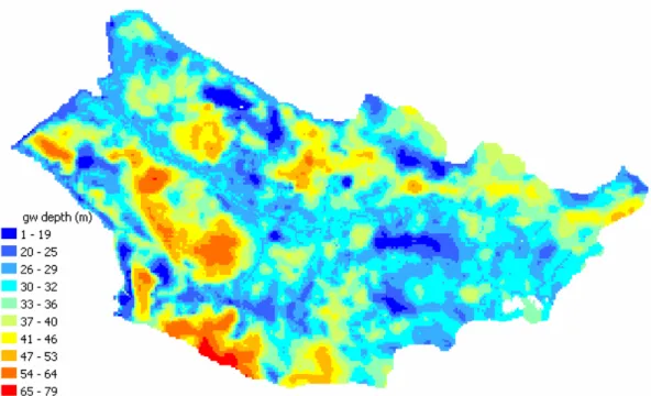
(from Météo-France). ... 72 Fig. 5.16 Hydraulic conductivity zones (from BRGM). ... 73 Fig. 5.17 Specific yield zones (from BRGM)... 73 Fig. 5.18 Groundwater depth (from BRGM). ... 74 Fig. 5.19 Initial transmissivity distribution on the modeled area... 75 Fig. 5.20 Initial specific yield distribution on the modeled area... 75 Fig. 5.21 Observed pumpage rates in the year 1995 by BRGM. ... 76

Fig. 5.22 Distribution of hydrometric and piezometric stations. ... 76 Fig. 5.23 The effect of the maximum value of infiltration (FN) on the flow measured at

Abbeville (catchment area = 5560 km2). ... 82 Fig. 5.24 The effect of depletion ratio of surface runoff reservoir (CQR)... 82 Fig. 5.25 The effect of the unsaturated model (NONSAT) run with a storage constant of τ

= 5 days. ... 82 Fig. 5.26 Calibration of parameters of Artificial Surfaces... 83 Fig. 5.27 Calibration of CRT and DCRT for Agricultural Zones... 83 Fig. 5.28 Evolution of measures of error; a) Deviation of runoff volumes (Dv), Root

mean squared error (RMSE); b) Correlation coefficient (ρ), Nash-Sutcliffe coefficient (R2), Coefficient of gain from daily mean (DG)... 84 Fig. 5.29 The variation of Nash-Sutcliffe coefficient (R2_{) for the Somme gauged at}

Abbeville and for its tributaries. ... 85 Fig. 5.30 Flow hydrograph of the Somme gauged at Abbeville (5560 km2) including the

validation period... 86 Fig. 5.31 Piezometric head distribution before the calibration of transmissivities. ... 87 Fig. 5.32 Piezometric head distribution after the calibration of transmissivities... 88 Fig. 5.33 The values of root mean squared error (RMSE) for piezometric heads before

and after the initial calibration of transmissivities... 90 Fig. 5.34 The Nash-Sutcliffe coefficients (R2_{) before and after the calibration of}

transmissivities. ... 90 Fig. 5.35 The root mean squared error (RMSE) values of piezometric heads before and

after the modification in specific yield. ... 91 Fig. 5.36 The rises applied to the elevations with the application of ‘fill’ procedure... 92 Fig. 5.37 Modification of river elevations in a cross-sectional view; a) application of

average slope line, b) modified elevations. ... 94 Fig. 5.38 Overflow depth in the center of the basin in year 2001; a) initial elevations, b)

after the application of ‘fill’ procedure, c) after correction of river elevations.95 Fig. 5.39 The effect of river elevation corrections on overflow depth and extent; a) before

correction, b) after correction. ... 97 Fig. 5.40 The root mean squared error (RMSE) values of piezometric heads before and

after the reassumption of initial specific yield values. ... 98 Fig. 5.41 The root mean squared error (RMSE) values of piezometric head fits before and

after the calibration of specific yield values... 99 Fig. 5.42 Final values of specific yield. ... 100

Fig. 5.43 The piezometric heads before and after the calibration of specific yield for the well 0335x0005. ... 101 Fig. 5.44 The piezometric heads before and after the calibration of specific yield for the

well 0625x0002. ... 102 Fig. 5.45 The Nash-Sutcliffe coefficients for piezometric head fits before (outer circles)

and after (inner circles) the calibration of specific yield. ... 102 Fig. 5.46 The final transmissivity values. ... 104 Fig. 5.47 The effect of transmissivity modification; dashed line represent the initial water table in which TA = TB = T, continuous line represent the water table after the

modification... 105 Fig. 5.48 Monthly flowrate of the Avre before and after the calibration of

transmissivities. ... 105 Fig. 5.49 Monthly flowrate of the Selle before and after the calibration of

transmissivities. ... 106 Fig. 5.50 The difference between the final and the previous transmissivity values, and

approximate flow directions. ... 106 Fig. 5.51 The piezometric head at the point numbered 0613x0012 before and after the

calibration of transmissivities... 107 Fig. 5.52 The difference between the final and the previous transmissivity values. ... 108 Fig. 5.53 The piezometric head hydrographs of a) 0474x0011 and b) 0478x0002 before

and after the calibration of transmissivities... 109 Fig. 5.54 The Nash-Sutcliffe coefficients for piezometric heads before (larger circles)

and after (smaller circles) the calibration; and for flowrates before (values in black) and after (values in red) calibration... 110 Fig. 5.55 The Nash-Sutcliffe coefficients of piezometric head fits before and after the

calibration of transmissivities... 110 Fig. 5.56 The effect of discharge coefficient on the Nash-Sutcliffe coefficients... 111 Fig. 5.57 The effect of the discharge coefficient on flow hydrograph of the Avre... 112 Fig. 5.58 The root mean squared error (RMSE) values of piezometric head fits before and

after the calibration of MODCOU... 114 Fig. 5.59 Measures of error before and after the calibration of MODCOU; a) Deviation

of runoff volumes (Dv), b) Root mean squared error (RMSE), c) Correlation coefficient (ρ), d) Nash-Sutcliffe coefficient (R2_{), e) Coefficient of gain from} daily mean (DG). ... 114 Fig. 5.60 Number of reservoirs in the Nash cascade... 116

Fig. 5.61 The effect of the storage constant, τ, on the Nash-Sutcliffe coefficients of flow hydrograph fits (the first test). ... 117 Fig. 5.62 Monthly averaged flowrate of the Somme at Abbeville between 1/1999 and

12/2001 for different values of the storage constant, τ (the first test)... 118 Fig. 5.63 The effect of the storage constant, τ, on the Nash-Sutcliffe coefficients of flow

hydrograph fits for the period 1/8/1985-31/7/2003 (the second test). ... 118 Fig. 5.64 The distribution of the values of storage constant, τ... 119 Fig. 5.65 The effect of NONSAT calibration on the Nash-Sutcliffe coefficients of the

Somme and its tributaries. ... 120 Fig. 5.66 The final results of simulations together with the calibration and validation

periods; (a)-(c) at various locations on the Somme, (d)-(g) on the tributaries of the Somme. ... 121 Fig. 5.67 Monthly discharges on the Somme at Abbeville for the period 1986-2002. .. 125 Fig. 5.68 Average annual discharge and baseflow... 125 Fig. 5.69 Comparison of total exfiltration depth in year 2001 calculated by MODCOU

(in blue) with a satellite derived image representing the flooded percentages of areas for the mesh given on April 21, 2001 when the flood reached its

maximum extent (in red). ... 126 Fig. 5.70 Comparison of total exfiltration depths excluding the river cells in year 2001

between MODCOU (in blue) and MARTHE (in red); a) downstream portion of the Somme, b) upstream portion of the Somme. ... 127 Fig. 5.71 The spatial distribution of exfiltration fluxes of year 2001 in the East-West

direction computed by; a) MARTHE, b) MODCOU. ... 129 Fig. 5.72 Flux exchange between the surface and the aquifer in the period

1/8/1985-31/7/2003... 130 Fig. 5.73 Effect of transmissivity and specific yield change on the average root mean

squared error obtained by using 50 head observation points... 132 Fig. 5.74 Effect of transmissivity and specific yield change on the average groundwater

level change obtained by using 50 head observation points... 132 Fig. 5.75 The effect of streambed conductance on flux exchange... 133

LIST OF SYMBOLS

AET : actual evapotranspiration

aC : calibration parameter for the CEQUEAU model

b : saturated thickness of aquifer

Cd : conductance of the drain

CQI : depletion ratio of the aquifer feeding reservoir

CQR : depletion ratio of the surface runoff reservoir

Criv : streambed conductance

CRT : mean value of soil water stock

Cd : discharge coefficient of the cell

Cds : discharge coefficient of the segment

Cred : redistribution coefficient

Dv : deviation of runoff volumes

DCRT : minimum value of soil water stock DG : coefficient of gain from daily mean

FN : maximum value of infiltration

g : gravitational acceleration

H0 : elevation of the water surface in the stream

h : piezometric head matrix

h : piezometric head

h0 : known value of piezometric head

K : hydraulic conductivity matrix

K : hydraulic conductivity

Kiz : number of isochronal zones

k : intrinsic permeability

kET : evapotranspiration coefficient

L : length of sand filter

l : length of a cell

N : number of reservoirs in the Nash cascade

Nk : number of cells inside the isochronal zone

n : number of grid cells with unknown piezometric head values

nr : number of river cells in the segment

nadj : number of adjacent cells

n : direction normal to the surface

P : precipitation

Pr : pumping rate

PET : potential evapotranspiration

Q : flow exchange with surface QC : constant flowrate value

Qmax : maximum infiltration rate QI : input of aquifer feeding reservoir

QImax : overflow level of aquifer feeding reservoir

QII : aquifer recharge

QR : input of surface runoff reservoir

QRmax : overflow level of the surface runoff reservoir.

QRR : surface runoff

Qaq : sum of the volume of water exchanged with the aquifer in the segment

Qr : sum of surface runoff volume flowing into the segment

Qw : volume of water outflowing from the balance reservoir

q : specific discharge

qlow : exchange of flowrate with the lower aquifer layer

qaq : volume of water exchanged between a river cell and the aquifer cell beneath

qr : surface runoff volume into a river cell

R : recharge rate

RMSE : root mean squared error R2 _{: Nash-Sutcliffe coefficient}

Raq : level of the aquifer feeding reservoir

Rb : level of balance reservoir

Rbmax : maximum level of balance reservoir

Rbnew : new level of balance reservoir

Rsur : level of the surface runoff reservoir

r : residue for convergence

S : storage coefficient

SCA : catchment area of the river cell

SW : area of the free water surface in the cell

Sc : confined storage

Ss : specific storage

Sy : specific yield

Sl : slope between two cells

T : transmissivity matrix

T : transmissivity

Tmax : maximum of transfer times

t : time

ttra : transition time

ttf : transfer time

V : volume of water in the cell

Vs : volume of water in the segment

α : constant of discharge time

β : calibration parameter for transition time calculation Δh : difference in piezometric heads

∆l : distance between the centers of two cells Δt : time step

Δtc : critical time step

ε : error limit

λmax : residue for overrelaxation factor μ : dynamic viscosity of water

ρ : correlation coefficient

ρw : density of water

τ : storage constant of reservoir

ω : overrelaxation factor

CHAPTER 1

I

NTRODUCTION 1. INTRODUCTION

1.1. Literature Survey

The interactions between groundwater and surface water have received considerable attention by many researchers. The problem of stream-aquifer interactions is important to watershed management efforts aiming at mitigating hazardous flood events, optimizing surface water and groundwater resources and also has significant ecological implications (Hantush et al. 2002). As Sophocleous (2002) points out, groundwater and surface water are not isolated components of the hydrologic system, but instead interact in a variety of physiographic and climatic landscapes. Thus, development or contamination of one commonly affects the other.

According to their relative position in space, Tóth (1963) defines three distinct types of flow systems: local, intermediate and regional, which could be superimposed on one another within a groundwater basin. In a local flow system, water flows to a nearby discharge area, such as a pond or stream. In a regional flow system, it travels a greater distance to major rivers, large lakes, or to oceans. An intermediate flow system is characterized by one or more topographic highs and lows located between its reach and discharge areas, but, unlike the regional flow system, it does not occupy both the major topographic high and the bottom of the basin.

Groundwater discharge is not only confined along the stream channel but also extends throughout the discharge area downgradient from the basin hinge line which is an imaginary line separating areas of upward (discharge) from downward (recharge) flow. Therefore, if baseflow calculations are used as indicators of average recharge, significant error may be introduced, because baseflow may represent only a relatively small part of the total discharge occurring downgradient from the hinge line (Sophocleous 2002).

Larkin and Sharp (1992) classify stream-aquifer systems as (1) underflow component dominated (the groundwater flux moves parallel to the river and in the same direction as the streamflow); (2) baseflow component dominated (the groundwater flux moves perpendicular to or from the river depending on whether the river is effluent or influent); (3) mixed. The dominant component can be deduced from geomorphologic data, such as, channel slope, river sinuosity, degree of river incision through its alluvium, the width-to-depth ratio of the bankfull river channel, and the character of the fluvial depositional system.

Sophocleous (2002) defines baseflow as water that enters a stream from persistent, slowly varying sources and maintains stream flow between water-input events. Subsurface flow can also enter streams quickly enough to contribute to the event response which is then called subsurface storm flow or interflow.

There are also researchers stressing the influence of the groundwater domain on hydrological basins. For example, Beven (2000) points out, one of the problems involved in having a complete understanding of hydrological systems is that most of the water flows takes place underground in the soil or bedrock and our ability to measure and assess subsurface flow processes is generally very limited.

1.2. Objective

The Somme river basin was influenced by a strong flood in year 2001 in which water levels reached to exceptional levels and caused an immense damage to the surroundings. This event has stressed the contribution of aquifers on the hydrology of basins. According to an estimation of BRGM (Bureau de Recherches Géologiques et Minières), nearly 75% of the flood volume was groundwater-induced as both exfiltration onto the surface and exchange between groundwater and river. The same event played an important role in the maintenance of discharges and causing attenuation of the consequences of dry seasons such as the spring and summer of 2003. Accordingly, in this research work a complete hydrogeological model of the Somme river basin in the north of France is aimed to be established with special emphasis on stream-aquifer interaction.

CHAPTER 2

T

HEORETICAL

B

ACKGROUND

F

OR

G

ROUNDWATER

F

LOW 2. THEORETICAL BACKGROUND FOR GROUNDWATER FLOW

In this chapter the principles of unsteady groundwater flow are described. While developing numerical methods for the analysis of field problems concerning groundwater flow, it is essential to build a mathematical model by defining the governing equations in the form of partial differential equations. These equations are considered as the mathematical representations of the physical phenomena occurring at a point in the flow domain (Aral 1990). The conceptual basis for the transient (or unsteady) fluid flow equation is the law of conservation of mass and Darcy’s law. In the following, a brief description of the groundwater flow equations is provided.

In 1856 Henry Darcy carried out experiments with sand-filled tubes for a water supply system for the city of Dijon, France (Darcy 1856). He discovered an important physical relationship in the science of porous-media hydrodynamics which is now called as

Darcy’s Law:

L h K

q=− Δ (2.1)

where q is the specific discharge or volumetric flowrate per unit area of porous medium,

K is the hydraulic conductivity of the porous medium, Δh is the difference in piezometric

head across the filter of length L, i.e. Δh=h₂ −h₁, as the piezometric head describes the sum of pressure head and potential head of the fluid, the term,

(

h2 −h1

)

L is to be

interpreted as hydraulic gradient along the flow path. By convention, the negative sign implies that flow is along the direction of decreasing gradient. The hydraulic conductivity is defined as:

μ

ρ g

k

K ₌ w

(2.2)

where k is the intrinsic permeability, ρw is the density of water, g is the gravitational acceleration, and μ is the dynamic viscosity of water.

Further information regarding the generalization or limitations of Darcy’s law can be found in Bear (1972), Delleur (1999) and Rushton (2003). Furthermore, sample values for the hydraulic conductivity and storage properties of unconsolidated and consolidated media are presented by Bear (1972), Bouwer (1978) and by Todd and Mays (2005). However, for actual models field investigations are essential.

Although it is common to use hydraulic conductivity in a general sense in describing the hydraulic properties of a porous medium, it is more advantageous to use the term, transmissivity to describe the ease with which water moves through a large porous medium such as a horizontal or layered aquifer. Transmissivity, T, is the product of hydraulic conductivity, K, and saturated thickness, b, of aquifer.

Kb

T = (2.3)

Transmissivity is defined in essentially horizontal flow as the discharge of water through the entire thickness of the aquifer per unit horizontal length of aquifer perpendicular to the direction of flow and per unit hydraulic gradient (Bear 1972).

In anisotropic porous media, where due to some direction related properties such as preferential lining of fractures, stratifications or layering, the conductivity changes depending upon direction (Delleur 1999). Such situations can be described by an extension of Darcy’s Law, where the hydraulic conductivity becomes a second order symmetrical matrix, K, with following components:

K (2.4) ⎥ ⎥ ⎥ ⎦ ⎤ ⎢ ⎢ ⎢ ⎣ ⎡ = zz yz xz yz yy xy xz xy xx K K K K K K K K K

where the quantities Kxx, Kxy and so forth are called the conductivity coefficients. Further,

in Cartesian coordinates, Darcy’s law becomes (Aral 1990):

z h K y h K x h K q_{x xx xy xz} ∂ ∂ − ∂ ∂ − ∂ ∂ − = (2.5) z h K y h K x h K q_{y xy yy yz} ∂ ∂ − ∂ ∂ − ∂ ∂ − = (2.6) z h K y h K x h K q_{z xz yz zz} ∂ ∂ − ∂ ∂ − ∂ ∂ − = (2.7)

where qx, qy and qz are the specific discharges in x, y and z directions, respectively.

As can be seen from Eqs. (2.5) to (2.7) potential gradients in one direction can yield flows in other directions. In practice, these equations are not much used, because it is not feasible to assess all conductivity components accurately. Whereas, in an anisotropic medium, where the principle hydraulic conductivity directions are parallel to the main coordinate directions chosen, the specific discharge vectors can be defined as:

x h K q_{x x} ∂ ∂ − = (2.8) y h K q_{y y} ∂ ∂ − = (2.9) z h K q_{z z} ∂ ∂ − = (2.10)

The specific discharge vectors constitute three of the four unknowns in a typical groundwater study. The remaining unknown is the piezometric head, h. Therefore a fourth equation is needed. The fourth equation is the continuity equation. Among different approaches, the most popular technique to derive the continuity equation is the representative elementary volume (REV) approach developed by Bear (1972), where macroscopic variables are defined as mean values over a REV. While the exact size of the REV is not determined, it is assumed that the size is much larger than the pore scale and much smaller than the scale of the porous medium. The results obtained with this approach yield macroscopic values for the groundwater flow, representing the average behavior of the fluid over the REV (Delleur 1999).

After employing the control volume approach, for a unit three-dimensional element, the following equation can be written:

t h S z h K z y h K y x h K x x y z s ∂ ∂ = ⎟ ⎠ ⎞ ⎜ ⎝ ⎛ ∂ ∂ ∂ ∂ + ⎟⎟ ⎠ ⎞ ⎜⎜ ⎝ ⎛ ∂ ∂ ∂ ∂ + ⎟ ⎠ ⎞ ⎜ ⎝ ⎛ ∂ ∂ ∂ ∂ (2.11)

where Ss is the specific storage of the aquifer assuming an elastic mechanical behavior for the REV.

Eq. (2.11) is the governing equation for unsteady three-dimensional groundwater flow in an anisotropic porous medium. However, due to practical reasons, that is, difficulty assessing the conductivity components correctly in all directions, a simpler mathematical model for multi-layered aquifers is rather preferred in the solution of groundwater problems. Eq. (2.11) is reduced to a quasi three-dimensional form by employing the following assumptions (Aral 1990):

1. The flow in the main aquifers is two-dimensional in the horizontal plane of the aquifer and the variation in the aquifer thickness is much smaller than the horizontal dimensions of aquifer. For an unconfined aquifer, this assumption is an extension to the well known Dupuit assumption, in which the vertical flow component is neglected and the potential lines are assumed to be vertical and the streamlines horizontal. The error introduced by this assumption is discussed by Bear (1972). In addition, solutions to two common groundwater problems with and without employing the Dupuit assumption are provided by Korkmaz and Önder (2006) and by Önder and Korkmaz (2007).

2. Main aquifer layers are hydraulically connected to each other by confining layers (aquitards). The direction of flow in the confining layers is vertical and the difference between the hydraulic conductivity of the main aquifers and the confining layers is large.

For a confined aquifer, Eq. (2.11) becomes

Q t h S y h T y x h T x x y c ∂ + ∂ = ⎟⎟ ⎠ ⎞ ⎜⎜ ⎝ ⎛ ∂ ∂ ∂ ∂ + ⎟ ⎠ ⎞ ⎜ ⎝ ⎛ ∂ ∂ ∂ ∂ (2.12)

where Sc is the confined storage and the term Q accounts for the flow exchange with surface as well as other aquifer layers.

For an unconfined aquifer (Fig. 2.1), Eq. (2.11) is reduced to

(

)

(

)

t h S P R y h z h K y x h z h K x x b y b r y ∂ ∂ = − + ⎟⎟ ⎠ ⎞ ⎜⎜ ⎝ ⎛ ∂ ∂ − ∂ ∂ + ⎟ ⎠ ⎞ ⎜ ⎝ ⎛ ∂ ∂ − ∂ ∂ (2.13)

where R is the recharge or injection rate from the surface, Pr is the pumping rate, Sy is the specific yield and the term

(

h−z_b

)

represents the thickness of the groundwater. R, Pr and

Q in Eq. (2.12) are defined in terms of volumetric flowrate per unit area.

zb

R Pr

h

impervious bottom FIG.2.1 Flow in a leaky unconfined aquifer.

In the solutions of certain problems in unconfined aquifer, some researchers as Bouwer et al. (1999) prefer to use transmissivity instead of hydraulic conductivity. In such cases, the product of hydraulic conductivity (K) with the average saturated thickness (h – zb) gives the transmissivity. When the vertical variations of the groundwater table are small compared to the saturated thickness, this is a useful assumption as it avoids the non-linearity of governing equation (Bear and Verruijt 1987). In this case a similar form of Eq. (2.12) is used.