Sub-stochastic matrix analysis for bounds
computation - theoretical results
Serge Haddad
aand Patrice Moreaux
baLAMSADE, UMR CNRS 7024, Université Paris Dauphine, Place du Maréchal de
Lattre de Tassigny, 75775 Paris, FRANCE, [email protected]
bLISTIC, Université de Savoie, BP 806, 74016 Annecy Cedex, FRANCE,
Abstract
Performance evaluation of complex systems is a critical issue and bounds computa-tion provides confidence about service quality, reliability, etc. of such systems. The stochastic ordering theory has generated a lot of works on bounds computation. Maximal lower and minimal upper bounds of a Markov chain by a st-monotone one exist and can be efficiently computed. In the present work, we extend simultaneously this last result in two directions. On the one hand, we handle the case of a maximal monotone lower bound of a family of Markov chains where the coefficients are given by numerical intervals. On the other hand, these chains are sub-chains associated to sub-stochastic matrices. We prove the existence of this maximal bound and we provide polynomial time algorithms to compute it both for discrete and continuous Markov chains. Moreover, it appears that the bounding sub-chain of a family of strictly sub-stochastic ones is not necessarily strictly sub-stochastic. We establish a characterization of the families of sub-chains for which these bounds are strictly sub-stochastic. Finally we show how to apply these results to a classical model of repairable system. A forthcoming paper will present detailed numerical results and comparison with other methods.
Key words: Markov process, Stochastic bound, Stochastic process, Strong stochastic ordering, Sub-Markov chain.
1 Introduction
Performance evaluation of complex systems [17,5,15] is a critical issue. Indeed since the development of such systems is expensive, an estimation of the re-quirements about their infrastructure is highly valuable for managers. Despite the continuous increasing of computers capacities, the exact analysis of huge
models is still out of reach. Alternative families of methods [19,12,16]. include simulations, approximations and bounds computations.
Bounds computation provides confidence about service quality, reliability, etc. In essence, the associated methods offer a trade-off between the accuracy of the bound and the complexity of its computation. Most of the proposed algorithms operate on Markovian processes either in the framework of Discrete Time Markov Chains (DTMCs) or in the one of Continuous Time Markov Chains (CTMCs).
Different theoretical analysis bounding methods [6,7,26,30,21,13,24,4] have been developed in order to derive efficient algorithms. Among these methods, the stochastic ordering theory [28,18] has generated numerous works including generic algorithms [2,11] and methods specific to particular applications [25]. Roughly speaking, this theory states that appropriate inequalities between the transition matrices (resp. the infinitesimal generators) of two discrete-time (resp. continuous-discrete-time) processes and their initial distribution lead to similar inequalities between their distribution at any time given that one of the process is of a special kind called monotone. Furthermore, the maximal lower and minimal upper bounds of a Markov chain by a monotone one exist and can be efficiently computed [29].
In the present work, we extend simultaneously this last result in two direc-tions. On the one hand, we handle the case of a maximal monotone lower bound of a family of Markov chains where the coefficients are given by nu-merical intervals. On the other hand, these chains are sub-chains associated
to sub-stochastic matrices. We prove the existence of this maximal bound and
we provide polynomial time algorithms to compute it for both DTMCs and CTMCs.
Moreover, the management of sub-stochastic matrices raises a new issue. A sub-chain is said strictly sub-stochastic iff given any initial distribution, the probability to indefinitely stay in the states of the sub-chain is null. It appears that the bounding sub-chain of a family of strictly sub-stochastic ones is not necessarily strictly sub-stochastic. So we have established an useful character-ization of the families of sub-chains fulfilling this property. This characteri-zation is qualitative in the sense that it depends on the transitions between states but not on the rates of these transitions.
Our third contribution is the application of the previous results to a generic model already studied by numerous authors. In the model, there is one state variable (e.g. the number of failed machines or the number of remote procedure calls) which induces a partition of states such that the steady-state probability mass quickly decreases w.r.t. this parameter. Moreover in a state transition the variable can arbitrarily increase whereas it can only decrease by one unit (e.g.
no simultaneous achievements of repair or call). This model admits a “bound-ing” model where the sets of states associated to values higher than some level are replaced by single states. The difficult step of this transformation is the computation of rates of the transitions starting from these aggregated states. Different solutions have been proposed [26,22,8,3]. The interest of the latter approach [3] is twofold : it covers realistic applications and the computation of bounding rates is straightforward. However due to drastic simplifications, the bounds can be really far from the exact values. We illustrate an application of our theory with a new solution method for this problem.
The balance of the paper is the following one. In the second section we de-velop a theory of bounds for families of sub-stochastic matrices of DTMCs. In section 3 we develop a similar theory for CTMCs. A significant example of application of these theoretical results is presented in section 4. At last, we conclude and summarize our results. Numerical experiments of these new methods will be detailed in a forthcoming paper.
2 Bounding sub-stochastic matrices of DTMCs
This section studies properties of sub-stochastic matrices of DTMC with one absorbing state when only bounds on these matrices are available. Such matri-ces are frequently encountered when analysing Markovian systems with large subsets of states of low probability.
2.1 Context and notations
We consider DTMCs X = (E, P(E)) on state space E = {1, . . . , n + 1}, where
n + 1 is the unique absorbing state. We study sub-stochastic matrices on C = {1, . . . , n}. In this section, all stochastic and sub-stochastic matrices
correspond to such DTMCs, thus: i) their (n + 1)th row, if any, is the (n + 1) row vector (0, . . . , 0, 1); ii) any n × n sub-stochastic matrix may be uniquely “extended” to a (n + 1) × (n + 1) stochastic matrix (the (n + 1)th column is defined to ensure that the extension is stochastic). Thus, in the rest of this section, a n × n sub-stochastic matrix will be viewed as it is or as its (n + 1) × (n + 1) absorbing extension, depending on the context.
We introduce the following notations:
• The restriction of a matrix L to rows in U and columns in V is denoted by
• For two vectors or matrices, usual comparison operators are taken
compo-nentwise.
• P− and P+, with P− ≤ P+ are two (n + 1) × (n + 1) positive matrices. P−
is assumed to be sub-stochastic.
• M(P−, P+) is the set of transition probability matrices of DTMCs X such
that P− ≤ P(E)≤ P+. We assume that M(P−, P+) 6= ∅.
There are several equivalent definitions of the strong stochastic ordering (≤st)
for DTMCs and stochastic matrices. However all these definitions are not appropriate to sub-chains comparison. Indeed, sub-chains comparison requires to use relations between terms of stochastic matrices involving summation of only n among n + 1 states of the chain. Since our subset corresponds to the first n states, we will use left to right summation in the definitions. Hence we rewrite standard definitions in this context.
Definition 2.1 (Strong stochastic ordering for stochastic matrices) Let A and B be n × m matrices (or vectors) with positive coefficients.
• A is st-monotone iff
∀ 1 ≤ i < j ≤ n, ∀ 1 ≤ k ≤ m, Pk
l=1A[i, l] ≥
Pk
l=1A[j, l].
• B is st-lower than A (denoted by B≤stA) iff
∀ 1 ≤ i ≤ n, ∀ 1 ≤ k ≤ m, Pk
l=1B[i, l] ≥
Pk
l=1A[i, l].
2.2 Existence and computation of an optimal st-lower bound P? of M(P−, P+)
In this section we prove the following theorem.
Theorem 2.2 Let P−, P+ be as above. There is an st-monotone matrix P? such that:
∀ P ∈ M(P−, P+), P?≤stP.
P? is st-maximal among st-monotone, st-lower bounds of M(P−, P+).
Moreover, P? can be built from P− and P+ in linear time w.r.t. their size (see
algorithms 1 and 2).
The proof is postponed until the presentation of the algorithm building P?.
2.2.1 Building P?
Building P?involves two steps. First we define a st-lower bound P•of M(P−, P+) starting from P− and P+. Then, P? is built from P• to be st-monotone.
Algorithm 1 first builds a matrix P(acc)where P(acc)[i, j] is the best computable upper bound of Σjk=1P[i, k] w.r.t. the inputs. Due to the second argument of
Algorithm 1 - Build P•
Input: P−, P+: (n + 1) × (n + 1) matrices
begin
for i ← 1 to n do
// compute the “accumulation” matrix P(acc): for j ← 1 to n do
P(acc)[i, j] ← minnPjk=1P+[i, k], 1 −Pn+1k=j+1P−[i, k]o
// (Ih) if i = j and P(acc)[i, j] = 1 then halt (see section 2.3)
endfor
// compute the bounding matrix P•: P•[i, 1] ← P(acc)[i, 1]
for j ← 2 to n do
P•[i, j] ← P(acc)[i, j] − P(acc)[i, j − 1]
endfor endfor end
the min function, P(acc)[i, n] ≤ 1 (note that P+ could be non stochastic). Then by “differentiating” this matrix we obtain P• which is a sub-stochastic
st-lower bound of any P ∈ M(P−, P+). The meaning of statement (Ih) will be explained in the handling of the strict sub-stochasticity (see theorem 2.6). For instance, if P+[i, .] = [0.2, 0.4, 0.5 0.3], P−[i, .] = [0.1, 0.15, 0.3 0.2]
(n = 3), we obtain P•[i, .] = [0.2, 0.15, 0.45].
Lemma 2.3 gives the key properties of P?.
Lemma 2.3 Let P• be the matrix computed by algorithm 1.
(1) P• is a st-lower bound of M(P−, P+), i.e., ∀ P ∈ M(P−, P+), P•≤
stP.
(2) P• belongs to M(P−, P+) i.e., P− ≤ P• ≤ P+.
Proof.
Assertion (1)
Let P ∈ M(P−, P+) and P(cum)[i, j] =Pj
k=1P[i, k].
Since P ≤ P+, P(cum)[i, j] = Pj
k=1P[i, k] ≤ Pj k=1P+[i, k] and as P− ≤ P, P[i, j] = 1 − Pn+1 k=j+1P[i, k] ≤ 1 − Pn+1
k=j+1P[i, k]. Hence P(acc)[i, j] ≥
P(cum)[i, j]. Assertion (2)
• For i = 1, P•[i, 1] def= P(acc)[i, 1] ≤ P+[i, 1], and since P•≤
stP, P•[i, 1] ≥
Algorithm 2 - Build a st-monotone version of a st-lower bound
Input: P• (see algorithm 1)
begin
P?[n, ·] ← P•[n, ·]
for i ← n − 1 downto 1 do (I0) x ← 0; y ← 0; ∆ ← 0 for j ← 1 to n do
(I1) P?[i, j] ← max {P•[i, j] − ∆, y + P?[i + 1, j] − x}
(I2) y ← y + P?[i + 1, j]
(I3) x ← x + P?[i, j]
(I4) ∆ ← ∆ + P?[i, j] − P•[i, j]
endfor endfor end
• For i > 1, P•[i, j]def= P(acc)[i, j] − P(acc)[i, j − 1]. We have P•[i, j] ≥ max{P(acc)[i, j]−Pj−1
k=1P+[i, k], P(acc)[i, j]−(1−
Pn+1
k=jP−[i, k])}.
If P(acc)[i, j] =Pj
k=1P+[i, k], taking the first term of the max we have P•[i, j] ≥
P+[i, j] ≥ P−[i, j]. If P(acc)[i, j] = 1−Pn+1
k=j+1P−[i, k], we take the second term
of the max and we have P(acc)[i, j] ≥ P−[i, j].
In the same way, P•[i, j] ≤ min{Pj
k=1P+[i, k]−P(acc)[i, j−1], 1−
Pn+1
k=j+1P−[i, k]−
P(acc)[i, j − 1]}.
If P(acc)[i, j − 1] = Pj−1
k=1P+[i, k], taking the first term of the min we have
P•[i, j] ≤ P+[i, j] and if P(acc)[i, j − 1] = 1 −Pn+1
k=j P−[i, k], we take the second
term of the min so that again P•[i, j] ≤ P−[i, j] ≤ P+[i, j]. 2
In the general case, P• built above is not st-monotone. So we now build a
monotone version P? of P•. Algorithm 2 is a “sub-stochastic version” of the
one proposed by [29,1]. It is based on the lemma 2.4 below.
Lemma 2.4 At the ith iteration of the outer loop and at the beginning of the
jth iteration of the inner loop of algorithm 2, one has the following equalities.
These equalities also hold for j = n + 1 with the meaning that the program is exiting the inner loop.
(1) y = Σj−1k=1P?[i + 1, k]
(2) x = maxnΣj−1k=1P•[i, k], yo= Σj−1
k=1P?[i, k] (3) ∆ = x − Σj−1k=1P•[i, k]
Furthermore the item P?[i, j] will take a positive value during the execution of
Proof.
We prove the lemma by induction on j.
For j = 1, the three equalities are due to statement (I0).
Let us suppose that we have proven the lemma until some value j. In order to analyze the effect of statement (I1), we substitute to y and ∆ the right-hand side of the equalities. This gives us:
P?[i, j] ← maxnΣj k=1P•[i, k] − x, Σjk=1P?[i + 1, k] − x o = maxnΣjk=1P•[i, k], Σj k=1P?[i + 1, k] o − x ≥ 0
The latter inequality is due to the first expression of x. The equality (1) is inductively proved due to statement (I2). Let us analyze the new value of x after statement (I3). We substitute to P?[i, j] the expression we have obtained
in our previous analysis. This gives us:
x ← maxn(Σjk=1P•[i, k], Σj
k=1P?[i + 1, k]
o
which is exactly the first expression of x. The second one is inductively proved by a simple examination of (I3).
Now we analyze the value taken by ∆ during the execution of statement (I4). We substitute the old value of ∆ by the expression of the third equality which gives us:
∆ ← x − Σj−1k=1P•[i, k] + P?[i, j] − P•[i, j] = Σj−1
k=1P?[i, k] − Σj−1k=1P•[i, k] +
P?[i, j] − P•[i, j].
The last equality has been obtained by the second expression of x in the second equality. 2
At first, algorithm 2 sets the last row of the new matrix to the same row of the old one. Then it sets each other row in decreasing ordering in such a way that a partial sum of the row is the least upper bound of the corresponding sum of the original matrix and the corresponding partial sum of the next row (which has already been set). The variable ∆ of the algorithm represents the excess of the current partial sum w.r.t. the original partial sum. The previous lemma (more precisely the second equality and the last assertion) proves that the transformed matrix is the minimal one satisfying the required property. It is straightforward that this new matrix is still a sub-stochastic matrix. Note that this algorithm could be implemented with a single matrix but we have chosen the current presentation in order to simplify the proof.
Suppose for example that (the (n + 1)th row is omitted)
P−= 0.3 0.3 0.2 0.1 0.1 0.2 0.3 0.2 0.1 0.0 0.2 0.2 0.1 0.2 0.1 0.1 0.0 0.2 0.1 0.2 , and P+= 0.5 0.5 0.5 0.5 0.2 0.4 0.4 0.4 0.4 0.2 0.4 0.4 0.4 0.4 0.2 0.3 0.3 0.3 0.3 0.2 .
Then algorithms 1 and 2 give: P(acc)= 0.3 0.6 0.8 0.9 0.4 0.7 0.9 1.0 0.4 0.6 0.7 0.9 0.3 0.5 0.7 0.8 , P•= 0.3 0.3 0.2 0.1 0.4 0.3 0.2 0.1 0.4 0.2 0.1 0.2 0.3 0.2 0.2 0.1 , and P? = 0.4 0.3 0.2 0.1 0.4 0.3 0.2 0.1 0.4 0.2 0.1 0.2 0.3 0.2 0.2 0.1 . 2.2.2 Proof of theorem 2.2
First, algorithm 2 ensures that P? is st-monotone. Moreover, the analysis of
the algorithm proved that P? is the greatest matrix monotone and
st-lower than P•.
Assume now that a st-monotone matrix A satisfies the relation of the theorem. Then A≤stP• since P• ∈ M(P−, P+) by assertion (2) of lemma 2.3, hence
A≤stP?.
Note that in fact the last column of P+ is not used to build P?.
2.3 Strict sub-stochasticity of P?
In order to deduce from P? bounds on the mean number of visits to states of
C before leaving C, P? must be strictly sub-stochastic.
Definition 2.5 (Strict stochasticity for stochastic matrices) A
sub-stochastic matrix P of a DTMC X is strictly sub-sub-stochastic iff whatever the starting state i in C, X will eventually leave C with probability 1.
This is equivalent to convergence of the series Pk≥1Pk.
Translating the definition in the graph theory context, we check strict sub-stochasticity of P?, in linear time w.r.t. the number of non null items of the
matrix, with the following procedure:
(1) Define an oriented graph where the set of nodes is I ∪ {n + 1} (2) There is an arc between i ∈ I and j ∈ I iff P?[i, j] 6= 0
(3) There is an arc between i ∈ I and n + 1 iff Σn
j=1P?[i, j] 6= 1
(4) Check whether n + 1 is reachable from any node. This can be done by a breadth-first backward search starting from n + 1.
The interested reader will find in [9] proof of the correctness of this algorithm. The important point here is that strict sub-stochasticity depends on structural criteria: whether an item is null and whether a row sum is 1. It would be interesting to have a similar structural characterization depending on P+ and
P− as it would give insight on which kind of rates bounds could be handled
by our method. This is the goal of the next theorem. Theorem 2.6 The following assertions are equivalent:
(1) P? is strictly sub-stochastic
(2) ∀i Pj≤iP•[i, j] < 1
(3) ∀i Pj≤iP+[i, j] < 1 or P
j>iP−[i, j] > 0
Consequently, P? is strictly sub-stochastic iff condition (Ih) of algorithm 1 is
never satisfied.
Proof.
The assertions 2 and 3 are equivalent due to the construction of P•. Thus we
will prove equivalence of 1 and 2.
At first, let us suppose that assertion 2 is satisfied. We claim that the same condition is satisfied for P?. We prove it by a reverse induction on i. If i = n
then it is immediate since the last rows of the two matrices are identical. Let us suppose that the inequalities are satisfied for the rows k > i. Then we know (see lemma 2.4) that:
P
j≤iP?[i, j] = max
nP j≤iP•[i, j], P j≤iP?[i + 1, j] o ≤
maxnPj≤iP•[i, j],P
j≤i+1P?[i + 1, j]
o
< 1
Thus in the graph associated to P? :
• eitherPj>iP?[i, j] = 0 and there is an arc from i to n + 1
• or Pj>iP?[i, j] > 0 and there is an arc from i to j > i
So starting from any node i and following these arcs, the node n + 1 will be eventually reached.
Now suppose that assertion 2 is not satisfied i.e.; ∃i Pj≤iP•[i, j] = 1. Thus
since P? is an adapted bound of P•, we have P
j≤iP?[i, j] = 1 and since
P? is monotone, ∀k ≤ iP
j≤iP?[k, j] = 1 holds. But this means that in the
associated graph of the above procedure, the subset of nodes {1, . . . , i} has no outgoing arc. Then n + 1 is unreachable from this subset of states. 2 Thus we directly check on the inputs whether our method is applicable. This is done without extra-computation by statement (Ih) of algorithm 1 which builds P•. Roughly speaking the criterion means that in the system, for any i there is either a j with j > i which any state of i can enter or i can exit C. More informally, the criterion states that if the ordering of the indices i
probability to progress. Of course, this does not preclude the probability of “regression”.
3 Bounding sub-generators of CTMCs
We follow an almost identical outline to the DTMC case to study properties of sub-generators of CTMCs with one absorbing state when only bounds on these matrices are available.
3.1 Context and notations
We consider CTMCs X = (E, P(E)) on state space E = {1, . . . , n + 1}, where
n + 1 is the unique absorbing state. We study sub-stochastic generators on C = {1, . . . , n}. A sub-generator is a n × n matrix Q such that: Q[i, j] ≥ 0
for i 6= j and Q[i, i] ≤ −Pj6=iQ[i, j]. In this section, all generators and sub-generators correspond to such CTMCs, thus: i) their (n+1)th row, if any, is the (n + 1) null row vector; ii) any matrix without explicit diagonal terms may be completed with adapted diagonal terms to be a generator (qi,i = −
P
j6=iqi,j);
iii) any n × n sub-generator may be uniquely “extended” to a (n + 1) × (n + 1) generator.
Given a (n + 1) × (n + 1) strictly upper triangular positive matrix Q− and a
(n + 1) × (n + 1) strictly lower triangular positive matrix Q+(hence diagonals of Q− and Q+ are undefined), M(Q−, Q+) is the set of generators of CTMCs
X = (E, Q(E)) where n + 1 is the unique absorbing state X and such that:
Q−≤ Q(E)u and Q(E)l ≤ Q+
with Q(E)
u and Q
(E)
l the strict upper triangle and the strict lower triangle of
Q(E).
Since we study sub-generators, we rewrite in this context the standard defini-tion of the strong stochastic ordering. This definidefini-tion is expressed differently in the full chains context [28].
Definition 3.1 (st-monotonicity of generators) A generator Q is st-monotone
iff, ∀ 1 ≤ i ≤ n, we have:
∀ 1 ≤ v < i, Pu≤vQ[i, u] ≥Pu≤vQ[i + 1, u],
∀ i < v ≤ n + 1, Pu≥vQ[i, u] ≤
P
Note that it is sufficient to compare two successive rows of Q to check if it is st-monotone.
Definition 3.2 (Strong stochastic ordering for generators) Let Q(1)and
Q(2)be two generators on E. Q(1)is st-lower than Q(2)(denoted by Q(1)≤
stQ(2)) iff, ∀ 1 ≤ i ≤ n :
∀ 1 ≤ v < i, Pu≤vQ(1)[i, u] ≥
P
u≤vQ(2)[i, u],
∀ i < v ≤ n + 1, Pu≥vQ(1)[i, u] ≤P
u≥vQ(2)[i, u].
As for DTMCs, st-relation between generators allows us to derive st-relation of their steady-state probabilities.
Theorem 3.3 ([28], Th. 4.2.8, p.67) Let X(1) and X(2) be two CTMCs on
{1, . . . , n} with generators Q(1) and Q(2) and probabilities vectors π(1)(t), π(2)(t)
at time t. Assume that ∀ 1 ≤ i < j ≤ n,
∀ 1 ≤ v < i, X u≤v qi,u(1) ≥ X u≤v qj,u(2) and ∀ j < v ≤ n, X u≥v qi,u(1) ≤ X u≥v qj,u(2)
Then for any initial probabilities vectors π(1)(0)≤
stπ(2)(0), we have π(1)(t)≤stπ(2)(t) for all t ≥ 0.
The first relation states that for any pair of states i ≤ j, the transition rate in X(1) to go to the set {1, . . . , v} with v < i from state i is bigger than the transition rate in X(2) to go to the same set from state j. Symmetrically, the second relation states that the transition rate in X(1) to go to the set
{v, . . . , n + 1} with v > j from state i is smaller than the transition rate in X(2) to go the same set from state j. Roughly speaking, X(1) is more likely to go backwards and X(2) is more attracted to go forwards. Thus, theorem 3.3 intuitively means that, given an initial distribution of X(1) more concentrated than X(2) on the subsets of states with small indices, at any time in the future the distribution of X(1) will still be more concentrated on such subsets. From theorem 3.3, we have immediately the corollary:
Corollary 3.4 Let Q(1)and Q(2)be two generators on E such that Q(1)≤
stQ(2).
If Q(1)is st-monotone then for any initial probabilities vectors π(1)(0)≤
stπ(2)(0),
we have π(1)(t)≤
3.2 Existence and computation of an optimal st-lower bound Q? of M(Q−, Q+)
In the same way as for DTMCs, we establish the following result.
Theorem 3.5 Let Q− and Q+ be as above. There is an st-monotone
gener-ator Q? such that:
∀ Q ∈ M(Q−, Q+), Q?≤
stQ.
Q? is st-maximal among st-monotone, st-lower bounds of M(Q−, Q+).
Q? can be built from Q− and Q+ in linear time w.r.t. their size (see
algo-rithm 3).
The proof is postponed until the presentation of the algorithm building Q?.
3.2.1 Building Q?
Let Q ∈ M(Q−, Q+). We restate conditions of theorem 3.3 in terms of matri-ces Q? and Q making a little transformation in the presentation which gives
the key idea of the construction:
∀ 1 ≤ i ≤ n, ∀ 1 ≤ v < i, X u≤v Q?[i, u] ≥ max i≤j≤n+1 X u≤v Q[j, u] , and ∀ 1 ≤ i ≤ n, ∀ i < v ≤ n + 1, X u≥v Q?[i, u] ≤ min i≤j<v X u≥v Q[j, u] .
With this set of inequalities, we build Q? row per row in decreasing ordering.
Row n + 1 is irrelevant since ∀ j, Q[n + 1, j] = 0. Thus we can set ∀ j, Q?[n +
1, j] = 0 and building this row will be skipped in the algorithm. We will use the bounding matrices Q− and Q+ in the construction of remaining rows of Q?.
Now looking for building row n and examining the above inequalities it ap-pears that only row n of Q is relevant. We must upper bound the partial sums “from the left” until the diagonal term (excluded) and lower bound the partial sums “from the right” until the diagonal term (excluded). This gives directly:
∀j < n, Q?[n, j] = Q+[n, j] and Q?[n, n + 1] = Q−[n, n + 1].
Algorithm 3 - Build Q?
Input: Q− an upper triangular (n + 1) × (n + 1) matrix,
Q+ a lower triangular (n + 1) × (n + 1) matrix
begin for j ← 1 to n − 1 do Q?[n, j] ← Q+[n, j] endfor Q?[n, n + 1] ← Q−[n, n + 1] Q?[n, n] ← −Pj6=nQ?[n, j] for i ← n − 1 downto 1 do x ← 0; y ← 0; ∆ ← 0 //lower triangle for j ← 1 to i − 1 do
Q?[i, j] ← max{Q+[i, j] − ∆, (y − x) + Q?[i + 1, j]}
∆ ← ∆ + (Q?[i, j] − Q+[i, j]) x ← x + Q?[i, j] y ← y + Q?[i + 1, j] endfor x ← 0; y ← 0; ∆ ← 0 //upper triangle for j ← n + 1 downto i + 2 do
Q?[i, j] ← min{Q−[i, j] + ∆, (y − x) + Q?[i + 1, j]} ∆ ← ∆ + (Q−[i, j] − Q?[i, j])
x ← x + Q?[i, j]
y ← y + Q?[i + 1, j] endfor
Q?[i, i + 1] ← Q−[i, i + 1] + ∆
//(Ih) if x + Q?[i, i + 1] = 0 then halt (see section 3.3)
Q?[i, i] ← −P
j6=iQ?[i, j]
endfor end
previous inequalities lead straightforwardly to the definitions:
∀ 1 ≤ v < i, X u≤v Q?[i, u] = max X u≤v Q+[i, u],X u≤v Q?[i + 1, u] , (1) ∀ i + 1 < v ≤ n + 1, X u≥v Q?[i, u] = min X u≥v Q−[i, u],X u≥v Q?[i + 1, u] ,(2) and X u≥i+1 Q?[i, u] = X u≥i+1 Q−[i, u]. (3)
algo-rithm 3. Statement (Ih) will be explained below (see theorem 3.8).
Note that building Q? indeed starts from the (n + 1) × (n + 1) matrix Q•,
“concatenation” of Q− and Q+. Lemma 3.6 Let Q• be the matrix:
∀ 1 ≤ i ≤ n, ∀ 1 ≤ j ≤ i, Q•[i, j] = Q+[i, j], ∀ i < j ≤ n + 1, Q•[i, j] = Q−[i, j], (i = n + 1), ∀ 1 ≤ j ≤ n + 1, Q•[n + 1, j] = 0.
(1) Q• is a st-lower bound of M(Q−, Q+), i.e., ∀ Q ∈ M(Q−, Q+), Q•≤
stQ.
(2) Q• belongs to M(Q−, Q+) i.e., Q−≤ Q• ≤ Q+.
The proof derives straightforwardly from the definitions.
3.2.2 Proof of Theorem 3.5
From (1), (2) and algorithm 3, Q? is st-monotone and it is the st-greatest
matrix among st-monotone, st-lower bounds of Q•.
Assume that matrix A is a st-lower bound of M(Q−, Q+). Then A≤
stQ•
since Q• ∈ M(Q−, Q+), hence A≤
stQ?.
3.3 Invertibility of Q?
|C
The second result is related to Q?
|C. The overall algorithm used for bounding
rates out of C (see section 4) includes the inversion of Q?
|C. Invertibility of
sub-generator indeed characterizes strict sub-stochasticity in the context of CTMCs.
Definition 3.7 (Strict sub-stochasticity for generators) A sub-generator Q of a CTMC X is strictly sub-stochastic iff whatever the starting state i in
C, X will eventually leave C with probability 1.
A necessary and sufficient condition for Q?
|C to be invertible, is that the
absorb-ing state n + 1 must be reachable from any other state [10]. Thus one checks in linear time w.r.t. the number of non null items of the matrix whether it is invertible with the following procedure:
(2) There is an arc between i ∈ C and j ∈ {1, . . . , n + 1} iff Q?[i, j] 6= 0
(3) Check whether n + 1 is reachable from any node. This can be done by a breadth-first backward search starting from n + 1.
The important point here is that non singularity depends on a structural criterium: whether an item is null or not. It would be interesting to have a similar structural characterization depending on Q+ and Q−. This is the goal
of the next theorem which shows that Q− is the single significant factor.
Theorem 3.8 The following assertions are equivalent:
(1) Q?
|C is invertible
(2) ∀i ∈ C Pn+1
j=i+1Q−[i, j] > 0
Consequently, Q?
|C is invertible iff condition (Ih) of algorithm 3 is never
sat-isfied.
Proof.
At first, let us suppose that the assertion 2 is satisfied. Then we know (see the introduction of this section) that: ∀i ∈ C Pn+1j=i+1Q?[i, j] =Pn+1
j=i+1Q−[i, j] >
0. Thus in the graph associated to Q?, given i ∈ C, there is an arc from i to
some j > i. So starting from any node i ∈ C and following these arcs the node
n + 1 will be eventually reached.
Now suppose that assertion 2 is not satisfied i.e., ∃i Pn+1
j=i+1Q−[i, j] = 0. Thus
by definition of Q?, we have ∀ k ≤ i, Pn+1
j=i+1Q?[k, j] = 0, but this means that
in the associated graph of the above procedure, the subset of nodes {1, . . . , i} has no outgoing arc. Then n + 1 is unreachable from this subset of states. Due to relation (3) above, the test in algorithm 3 actually corresponds to the second assertion. 2
Thus we directly check on the inputs whether our method is applicable. This is done without extra-computation by the instruction (Ih) of the algorithm 3. It should be emphasized that this criterion is really close to the one of the discrete time case.
We may derive from the method used to compute lower bounding rates, a similar approach to compute upper bounding rates out of C. Without provid-ing technical details, let us point out that this can be achieved by definprovid-ing a st-monotone and upper bound of matrices Q, starting from matrices Q+ (a upper-triangular matrix, and Q− (a lower-triangular matrix). Note that
de-spite similar notations, these matrices are not the same ones as the matrices of the previous paragraph.
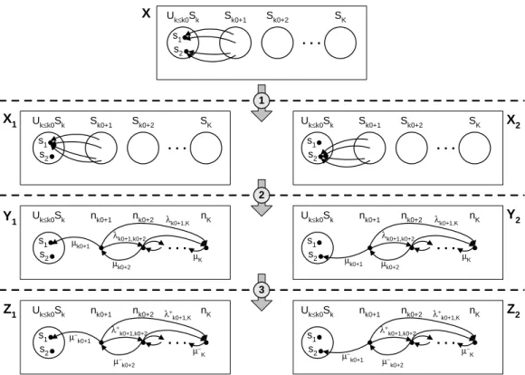
. . . s1 s2 Uk≤k0Sk Sk0+1 Sk0+2 SK X1 . . . s1 s2 Uk≤k0Sk Sk0+1 Sk0+2 SK X2 . . . s1 s2 Uk≤k0Sk Sk0+1 Sk0+2 SK X . . . s1 s2 Uk≤k0Sk nk0+1 nk0+2 λ+k0+1,K nK Z2 µ− k0+1 λ+ k0+1,k0+2 µ− k0+2 µ− K . . . s1 s2 Uk≤k0Sk nk0+1 nk0+2 λ nK Y2 k0+1,K µk0+1 λk0+1,k0+2 µk0+2 µK . . . s1 s2 Uk≤k0Sk nk0+1 nk0+2 nK Z1 λ+ k0+1,K µ− k0+1 λ+ k0+1,k0+2 µ− k0+2 µ− K . . . s1 s2 Uk≤k0Sk nk0+1 nk0+2 nK Y1 λk0+1,K µk0+1 λk0+1,k0+2 µk0+2 µK 1 2 3
Figure 1. From bounds on rates to bounds on steady-state probabilities
4 Applications to reward bounding
Results established in sections 2 and 3 aim to devise bounds of rewards on subsets of DTMCs or CTMCs with small steady-state probability. In a forth-coming paper (see [14] for a first set of results) we will provide various appli-cations of these results to DTMCs as well as to CTMCs. In this section, we only give an overview of the approach for bounding output rate of a subset of a CTMC, a problem already studied by several authors, especially in the context of reliabity/performability of systems. We first describe the general approach, based on the polyhedral method of Courtois and Semail [6] and on stochastic bounds. Then we give the sketch of our method to provide lower bounds of output rates from aggregates of states involved in this approach.
4.1 Bounding steady-state distribution in large CTMCs
As stated in the introduction, we would like to develop an a priori (i.e. from the model parameters) aggregated Markov chain on the irrelevant states w.r.t. the probability distribution in order to reduce the combinatory explosion in-duced by complex systems. Ideally the steady-state probability of the rein-duced chain should be the aggregation of the original steady-state probability. Such a chain exists and is called the exact aggregation of the original chain. However
A µ(A) B Ci C1 Cn C
(a) Initial sub-chain
n+2 B n+1 A C = {1, 2, ..., n} (b) Aggregated sub-chain Figure 2. Aggregation around a subset C
since rates between aggregated states Si involve computation of the original
steady-state probability (i.e. qi,j = π(Si)−1· Σs∈Siπ(s) · Σs0∈Sjqs,s0), this exact
aggregation seems to be useless.
Fortunately in some typical cases, knowing bounds on these rates is sufficient to deduce bounds on the steady-state probabilities. As one of the possible applications of our work is a better handling of such cases, we briefly describe in figure 1 a generic model and the appropriate bounding algorithm. In the model, there is one state variable (e.g. the number of failed machines or the number of remote procedure calls) which induces a partition of states S =
UK
k=1Sksuch that the probability mass quickly decreases w.r.t. this parameter.
Moreover in a state transition the variable can arbitrarily increase whereas it can only decrease by one unit (e.g. no simultaneous achievements of repair or call). Following the notations of the figure, we informally justify the method (see the references for a more detailed presentation).
(1) Given a subset of states, we substitute a Markov chain (MC) X for a family of MC Xi indexed by the entry points of the subset where in each Xi, all entries in the subset are redirected to si. Then the steady-state
probability of X is a barycenter of the family of steady-state probabilities corresponding to Xi (see [6,7]).
(2) The second step is simply the application of the exact aggregation on Xi
producing Yi such that the steady-state probability vector restricted to
Uk0
k=1Sk in the MC Xi is identical to the corresponding vector in Yi
(3) The last step is specific to this kind of MC and states that the steady-state probability vector restricted to Uk0
k=1Sk in the MC Zi is a lower
bound of the corresponding vector in Yi if ∀i, j λ+i,j ≥ λi,j and µ−i,j ≤ µi,j
(see [26,20]).
Summarizing the method, we first obtain bounds on the firing rates by a structural analysis of the model, then we compute steady-state probabilities of MCs Zi and finally we deduce a lower bound of the probability vector of
the original MC restricted to Uk0
4.2 Lower bounding output rate of a subset of states
Let us concentrate on bounding the rate out of subsets using only the param-eters of the model and not using the whole CTMC.
In order to structurally bound the rates, different solutions have been pro-posed: the simplest solution [26] consists in taking λ+
i,j = maxs0∈Si n Σs”∈Sj qs0,s” o and µ−i = mins0∈S i n Σs”∈Si−1 qs0,s” o
. Such a solution has a serious drawback: in numerous models µ−i = 0 which forbids the use of the method. Alternatively in particular cases [22], analytical expressions can be found for a general lower bound of µ−
i , but the application area is still very limited. At last, Carrasco [3]
has proposed a general solution when activities inside the Sk subsets
corre-spond to special phase-type distributions. The interest of the latter approach is twofold : it covers realistic applications and computation of bounding rates is straightforward. However due to drastic simplifications, these lower bounds can be really far from the exact values.
Let us consider a given subset Si, renamed as C in the sequel to make easier the
link with results of section 3. Our method is based on the main hypothesis that
C can be partitioned into subsets Ci and that bounds on cumulated rates from
a state to some Ci can be obtained by a structural analysis of the model. Such
a situation is illustrated in figure 2: the chain will eventually jump from C to
A or to B (figure 2a). The sets are aggregated as C = {1, . . . , n}, A = {n + 1}
and B = {n + 2} (figure 2b). Examples of the application paper will show that these are weak restrictions and moreover that often different partitions are possible where the choice of the appropriate partition is a trade-off between accuracy of the bounds and complexity of the computation.
In the sequel, D = CS{n + 1, n + 2}, X = (D, Q(D)) is the aggregated CTMC with unique absorbing states n + 1 and n + 2. Let µn+1 be the output rate
from C to A. The successive steps of our bounding method for µn+1 are the
following.
1. In the CTMC X, we have:
µn+1 =
p(C)n+1 h(C)
where p(C)n+1 is the steady-state probability to reach n + 1 when leaving C and
h(C) is the holding time of X in C.
next equations relate the previous quantities (see for instance [27,23]): p(C)n+1 = n X i=1 αip(i)n+1 and h(C)= n X i=1 αih(C,i).
p(i)n+1 is the steady-state probability to reach n + 1 when leaving C, starting from i, and h(C,i) is the holding time in C, when entering C in i.
3. We deduce that: µn+1= n X i=1 αih(C,i) Pn i=1αih(C,i)
(p(i)n+1/h(C,i)) ≥ min
i
p(i)n+1
h(C,i). (4)
So in the sequel, we focus on lower bounding p(i)n+1 and upper bounding h(C,i). 4. Lower bound of p(i)n+1.
Let P be the transition matrix of the embedded DTMC of X. We obtain the probability p(i)n+1 to leave C for n + 1, when starting from i by conditioning this probability on the number of transitions before leaving C. Thus:
p(i)n+1 =X j≤n X k≥0 (P|C)k [i, j] × P[j, n + 1].
Let us assume that we know a (n + 1) × (n + 1) matrix P− ≤ P. Since the
right-hand side of the above equation is composed by positive terms, sums and products, we only have to lower bound each item of this expression by the corresponding item of P− in order to obtain a lower bound of p(i)
n+1.
5. Upper bound of h(C,i).
Let us denote by X(C) = (E, Q(E)) the CTMC X restricted to E and with output rates to states n+1 and n+2 merged: Q(E)is (n+1)×(n+1) and its last column is the sum of last two columns of Q(D). If π(C,i)(t) is the probability distribution of X(C) at time t with initial distribution π(C)(0) = 1
i, i.e. with X(C) starting in i, then by definition:
h(C,i) = +∞ Z 0 X j∈C π(C,i)(t)[j]dt.
Due to the aggregation procedure, Q(E)cannot generally be computed without solving the whole (large) CTMC. However in several cases, like repairable systems for instance, componentwise (triangular) bounding matrices Q− and
we can apply results of section 3. If Y = (E, Q?) we get: h(C,i)Y = ∞ Z 0 X j≤n πY(C,i)(t)[j] dt ≥ ∞ Z 0 X j≤n π(C,i)(t)[j] dt = h(C,i)
where π(C,i)Y (t) is the probability distribution of Y at time t with initial dis-tribution πY(C)(0) = 1i.
Finally, we know that in a CTMC (E, Q) with n+1 as unique absorbing state, the vector h of holding times hi in C starting from i satisfies: −Q|C· h = 1Tn,
1T
n being the n row vector of 1. Thus, if the matrix Q?|C is non singular (see
theorem 3.8), we define upper bounds for holding times as: h+ = −³Q?
|C
´−1
· 1T
n (5)
Full details of the method and numerical results will be presented in a paper dedicated to applications. We simply note here (see the report [14]) that com-parisons of this method with the one presented in [3] have shown that these bounds are significantly better with a manageable extra-cost of computation.
5 Conclusion
Computation of bounds is known to be useful for managing some strategic choices with a high degree of confidence. The stochastic ordering theory [28] has generated numerous works related to such computations. Motivated by bounding steady-state averaged rewards of subsets of states of a large Markov chain, we have enlarged some features of this theory in order to handle the case of a maximal monotone lower bound of a family of Markov sub-chains where the coefficients are given by numerical intervals. We have proved the existence of this maximal bound and we have provided polynomial time algorithms to compute it for both DTMCs and CTMCs.
Moreover, we have solved a specific problem, i.e. we have characterized the families of sub-chains whose maximal lower bound is strictly sub-stochastic. In order to give an insight to the applicability of our results, we have revisited a bounding method for a standard model of Markov chain.
In a forthcoming paper we will present several applications of these results in the discrete case as well as in the continuous case. The paper will include de-tailed numerical results and comparisons with other approaches. In particular, we will show that, with low computation overhead, application of our results
to a repairable Markov model gives significantly better bounds that the ones obtained by the method presented in [3].
References
[1] O. Abu-Amsha and J.M. Vincent. An algorithm to bound functionals of Markov chains with large state space. Rapport MAI 25, IMAG, Grenoble, France, April 1996.
[2] O. Abu-Amsha and J.M. Vincent. An algorithm to bound functionals of Markov chains with large state space. In Proc. of the 4th INFORMS Conference on Telecommunications, Boca Raton, 1998.
[3] J.A. Carrasco. Bounding steady-state availability models with group repair and phase type repair distributions. Performance Evaluation, 35:193–214, 1999. [4] J.A. Carrasco. Handbook of Reliability Engineering, chapter Markovian
dependability/Performability modeling of fault-tolerant systems, pages 613–642. Springer–Verlag, 2003.
[5] C.G. Cassandras. Discrete Event Systems: Modeling and Performance Analysis. Irwin Pub., 1993.
[6] P. J. Courtois and P. Semal. Bounds for the positive eigenvectors of nonnegative matrices and for their approximations by decomposition. Journal of ACM, 31(4):804–825, October 1984.
[7] P. J. Courtois and P. Semal. Computable bounds on conditional steady-state probabilities in large markov chains and queueing models. IEEE Journal on Selected Areas in Communication (SAC), 4(6):926–937, September 1986. [8] S. Donatelli, S. Haddad, P. Moreaux, and M. Sene. Bounds for rewards of
systems with clients/servers interactions. In W. J. Stewart B. Plateau and M. Silva, editors, Proc. of the third International Workshop on Numerical Solution of Markov Chains, pages 208–227, Zaragoza, Spain, September 8–10 1999. Prensas Universitarias de Zaragoza. .
[9] W. Feller. An introduction to probability theory and its applications. Volume I. John Wiley & Sons, 1968. (third edition).
[10] W. Feller. An introduction to probability theory and its applications. Volume II. John Wiley & Sons, 1971. (second edition).
[11] J.M. Fourneau and N. Pekergin. An algorithmic approach to stochastic bounds. In M. Calzarossa and S. Tucci, editors, Performance Evaluation of Complex Systems: Techniques and Tools, Performance 2002, Tutorial Lectures, number 2459 in LNCS, pages 64–88, Rome, Italy, September 22–27 2002. Springer– Verlag.
[12] E. Gelenbe, editor. System Performance Evaluation: Methodologies and Applications. CRC Press, March 2000.
[13] L. Golubchik and John C.S. Lui. Bounding of performance measures for a threshold–based queueing system with hysteresis. In ACM Sigmetrics International Conference on measurement & modeling of computer systems, volume 25 of Performance Evaluation Review, special issue, pages 147–157, Seattle, Washington, USA, June 15-18 1997. ACM.
[14] S. Haddad and P. Moreaux. Sub-stochastic matrix analysis and performance bounds. Research Report RAP-CReSTIC-1, CReSTIC, Université de Reims Champagne-Ardenne, France, October 2004. .
[15] G. Haring, Ch. Lindemann, and M. Reiser, editors. Performance Evaluation: Origins and Directions, volume 1769 of LNCS. Springer–Verlag, 2000.
[16] B.R. Haverkort, R. Marie, G. Rubino, and K. Trivedi, editors. Performability Modelling : Techniques and Tools. Wiley, Chichester, England, 2001.
[17] R. Jain. The art of computer systems performance analysis. John Wiley & Sons, 1991.
[18] M. Kijima. Markov processes for stochastic modeling. Stochastic modeling. Chapman and Hall, London, UK, 1997.
[19] A.M. Law and W.D. Kelton. Simulation modeling and analysis (3rd ed.). MacGraw-Hill, New-York, 2000.
[20] J.C.S. Lui and R.R. Muntz. Computing bounds on steady state availability of repairable computer systems. Journal of ACM, 41(4):676–707, July 1994. [21] J.C.S. Lui, R.R. Muntz, and D. Towsley. Bounding the mean response time of
the minimum expected delay routing policy: an algorithmic approach. IEEE Transactions on Computers, October 1994.
[22] S. Mahévas. Modèles markoviens de grande taille : calculs de bornes. Thèse, Université de Rennes I, IFSIC, December 18 1997.
[23] S. Mahévas and S. Rubino. Bound computation of dependability and performance measures. IEEE Transactions on Computers, 50(5):399–413, 2001. [24] S. Majumdar and C.M. Woodside. Robust bounds and throughput guarantees for closed multiclass queueing networks. Performance Evaluation, 32(2):101– 136, March 1998.
[25] M. Ben Mammoun, J. M. Fourneau, N. Pekergin, and A. Troubnikoff. An algorithmic and numerical approach to bound the performance of high speed networks. In Proc. of the 10th Int. Workshop on Modeling, Analysis and Simulation of Computer and Telecommunication Systems (MASCOTS 2002), pages 375–382, Fort Worth, Texas, USA, October 11–16 2002.
[26] R.R. Muntz, E. De Souza E Silva, and A. Goyal. Bounding availability of repairable computer systems. In Proceedings of 1989 ACM SIGMETRICS and PERFORMANCE’89, May 1989. also in special issue of IEEE Trans. Computers, vol. 38, no. 12, pp. 1714-1723, Dec. 1989.
[27] G. Rubino and B. Sericola. Sojourn times in finite Markov processes. Journal of Applied Probability, 27:744–756, July 1989.
[28] D. Stoyan. Comparison Methods for Queueing and Other Stochastic Models. John Wiley & Sons, 1984.
[29] M. Trémolière, J.M. Vincent, and B. Plateau. Determination of the optimal upper bound of a Markovan generator. Technical Report 106, LGI–IMAG, Grenoble, France, 1992.
[30] N.M. van Dijk. The importance of bias terms for error bounds and comparison results. In W. J. Stewart, editor, Proc. of the First International Workshop on Numerical Solution of Markov Chains, Raleigh, NC, USA, January 8–10 1990. Marcel Dekker, NY, USA, 1991.