Risk Shifting, Asset Bubbles, and Self-fulfilling Crises

Risk Shifting, Asset Bubbles,

and Self-ful…lling Crises

Edouard Challe and Xavier Ragot

Abstract

Financial crisis are often associated with an endogenous credit reversal fol-lowed by a fall in asset prices and failures of …nancial institutions. To account for this sequence of events, this paper constructs a model where the excess risk-taking of portfolio investors leads to a bubble in asset prices (in the spirit of Allen and Gale, Economic Journal, 2000), and where the supply of credit to these investors is endogenous. First, we show that changes in the composition and riskiness of investors’portfolio as total lending varies may cause the ex ante return on loans to increase with the amount of total lending, thereby creating the potential for multiple (Pareto-ranked) equilibria associated with di¤erent levels of lending, asset prices, and output. We then embed this mechanism into a 3-period model where the low-lending equilibrium is selected with positive probability at the intermediate date. This event is associated with a ine¢ cient liquidity dry-up, a market crash, and widespread failures of borrowers.

Keywords: Credit market imperfections; self-ful…lling expectations; …nancial crises.

JEL codes: G12; G33.

CNRS, DRM-CEREG, Université de Paris-Dauphine, Place du Maréchal de Lattre de Tassigny, 75775 Paris Cedex 16; email: edouard.challe@dauphine.fr.

y_{CNRS, Paris-Jourdan Sciences Economiques, 48 bd Jourdan 75014 Paris; email:}

1

Introduction

The resurgence of …nancial crises in the …fteen years, both in OECD and emerg-ing contries, has sparked a renewal of interest in the potential sources of …nancial fragility and market imperfections in which they originate. Although each crisis had, of course, its own speci…cities (depending, in particular, on the variety of exchange rate regimes that were adopted), it is now widely agreed that they all were charac-terised by a typical underlying pattern involving destabilising developments in credit and asset markets. Amongst OECD countries in the 80s and early 90s, like Japan or Scandinavian countries, …nancial crises were an integral part of a broader ‘credit cycle’, whereby …nancial deregulation led to an increased amount of available credit, fulled a period of overinvestment in real estate and the stock market, leading to ex-cessive asset-price in‡ation. These events were then followed by a credit contraction (or ‘crunch’), the bursting of the asset bubble, causing the actual or near bankrupcy of the …nancial institutions which had previously borrowed to buy them (see Borio et al. (1994), Allen and Gale (1999) for a more detailed account of these events). In many emerging countries, particularly in Asia and Latin America, capital account lib-eralisation allowed large in‡ows of capital, with a similar e¤ect of raising asset prices to unsustainable levels; This phase of overlending usually ended in a brutal capital account reversal from large de…cits to small ones (or sometimes small surpluses), ac-companied by a market crash and a banking crisis, also often (but not necessarily) coupled with the collapse of the prevailing exchange rate regime (see Kaminsky and Rheinart (1998, 1999), and Calvo (1998) for the evidence on this typical pattern, sometimes referred to as ‘sudden stop’).

An important theoretical issue, yet largely unsanswered, is whether the credit reversal that typically accompanies such crisis is the outcome of an autonomous, ex-trinsic, reversal of expectations on the part of economic agents, or simply the natural outcome of building up macroeconomic imbalances and/or policy mistakes, i.e., the intrinsic fundamentals of the economy. For a time, it has been fashionable to inter-pret …nancial crisis as the mere outcome of extraneous ‘sunspots’hitting the beliefs of investors, regardless of the underlying fundamental soundness of the economy. For example, early models of banking crises would emphasise the inherent instability of the banking system, whose provision of liquidity insurrance made them sensitive to self-ful…lling runs, as the ultimate source of vulnerability to crises (see Diamond and Dybvig (1983), and Chang and Velasco (2000) for an open economy version of a

sim-ilar model). In a simsim-ilar vein, ‘second-generation’ models of currency crisis would insist on the potential existence of multiple equilibria in models of exchange rate determination, where the defense of a pre-announced peg by the central bank is too costly to be fully credible –see, for example, Velasco (1996) and Obsfeld (1996)).

Although expectational factors certainly play a rôle in triggering …nancial crises, theories based purely on self-ful…lling expectations clearly do not tell the full story. In virtually all the recent episodes that we just brie‡y refered to, speci…c macroeconomic or structural sources of fragility preceded the actual occurrence of the crisis. In OECD countries, for example, …nancial crises usually followed periods of excessively loose monetary policy and/or poor exchange rate management (see Borio et al. (1994)). In emerging countries, the culprit was often to be found in the weakness of the banking sector due to poor …nancial regulation, as well as other factors such as unsustainable …scal or exchange rate policies (Summers (2000)). In the speci…c case of emerging countries crises, the empirical evidence clearly indicates that, while indicators of fundamental weaknesses clearly explain a large part of the probability that a crisis will occur, a sizeable non fundamental component remains (see Kaminsky (1999), as well as the discussion of this piece of evidence by Chari and Kehoe (2003)). We interpret such evidence as suggesting that both aspects (fundamental and ‘extrinsic’) are at work when a …nancial crisis triggers, and that both ingredients should be part of any theoretical model trying to explain the recent crisis episodes in developed and developing countries.

The present paper aims to o¤er a model of this kind. We draw on Allen and Gale’s (2000) (AG in the remainder of the paper) theory of …nancial crises, which in our view best grasps a central feature of all recent crisis, i.e., a credit-fulled asset bubble, followed by a market crash and the failures (or near-failure in case of government bail-out) of the …nancial institutions that had borrowed to buy speculative assets. In AG, …nancial crises are the natural outcome of credit relations where portfolio investors borrow to buy risky assets, and are protected against a bad realisation of the asset payo¤ by the use of simple debt contract with limited liability. Investors’ twisted incentives then lead them to overinvest in the risky asset (risk shifting), whose price consequently rises to high levels (asset bubble), with the possibility that they go bankrupt if the asset payo¤ turns out badly (…nancial crisis). While AG focus on the ‘partial equilibrium’case where the total amount of credit available to portfolio investors is exogenous, we allow the supply of credit to vary according to an optimal consumption-savings plan by lenders. We regard this alternative assumption

as not only more realistic, but also particularly relevant to the recent crises, where the endogeneity of the credit supply was frequently blamed for being an important cause of …nancial instability.

Analysing the interdependence between individual savings decisions by lenders and the equilibrium return on loans to investors turns out to yield a whole new set of predictions, which can be summarised as follows. Within a two-period model of lending and portfolio choice, we …rst show that variations in aggregate lending to investors alters the composition and riskiness of their portfolio, and thus the return that are able to o¤er in equilibrium, in a possibly non-monotonic way. On the one hand, a higher level of aggregate savings raises productive investment, with the stan-dard e¤ect of reducing marginal productivity and the equilibrium loan return. On the other hand, higher savings tend to aleviate the risk shifting problem by reducing the proportion of investors’resources that are invested in the risky asset, and thus the average riskiness of investors’portfolio. This second, non-standard e¤ect goes against the standard one as it tends to increase the per unit return on loans. Under certain circumstances that we specify below, it is strong enough to more than o¤set the …rst one, causing the ex ante loan return to increase with the amount of total lending. Coupling this phenomenon with a simple speci…cation for the endogenous savings behaviour of lenders, the possible increasingness of the loan return function creates a strategic complementarity in lending decisions, which may in turn give rise multiple equilibria associated with di¤erent levels of lending, interest rates, and asset prices. Importantly, the possibility that multiple equilibria exist is shown to be related to the severity of the risk-shifting problem in the economy, such as implied by the payo¤ risk associated with holding the risky asset. Finally, we show that these multiple lending equilibria are unambiguously Pareto-ranked; the lower aggregate lending, the lower asset prices (i.e., the higher interest rates), and the lower aggregate welfare. A coordination failure may thus occur if lenders collectively choose a stable level of aggregate lending that has poor welfare properties.

To go from a theory of multiple equilibria in credit and asset markets to one of self-ful…lling crises, our next step is embed the mechanism that we just described into a three-period, stochastic model where the low-lending equilibrium is selected with positive probability at the intermediate date. The interpretation of this event is that a ‘sunspot’, i.e. an extraneous signal on which agents coordinate their expec-tations, lead them to believe that the community of lenders as a whole will select the equilibrium with low lending at date 1. This event is associated with a self-ful…lling

liquidity dry-up, as lenders remove a large amount of funds from the portfolio invest-ment sector, accompanied by a …nancial crisis, i.e., the failure of those investors who had borrowed to …nance their portfolio investment. More speci…cally, we show that such crises have the following characteristics; i) lending to portfolio investors drops down as lenders choose to consume, rather than save, a large share of their endow-ment of goods, ii) this causes a fall in investors’…nancial resources and a drop in the demand for risky assets, whose price consequently falls to low levels, and iii) this fall in asset prices forces into bankruptcy investors who have previously borrowed to buy them, as the total value of their assets falls short of their liabilities. To summarise, …nancial crises are associated with a sudden credit contraction, followed by a market crash and widespread failures of borrowers. Importantly, such crises follow a rever-sal of expectations on the part of lenders and are not restricted to situations where uncertainty about the amount of available credit is induced by policy (as in times of uncertain …nancial liberalisation, the example emphasised by AG). Again, and for the same reason as in the two-period model, self-ful…lling crises are more likely to occur in economies where the risk shifting problem, and the associated excessive risk-taking by borrowers, is severe.

Our model of self-ful…lling …nancial crises also turns out to have interesting welfare implications, which do not duplicate the welfare properties of the possible (determin-istic) equilibria of the two-date model. First, the drop in asset prices that follows the occurrence of the crisis at the intermediate date generates negative wealth e¤ects on lenders budget set, which forces them to cut their discounted consumption ‡ow, and thus their ex ante welfare, from then on. Second, the reduction in aggregate savings that follows lowers productive investment, with the consequence of lowering entrepreneurs’consumption and welfare. Then, the higher the ex ante probability of a crisis, the most likely these poor outcomes, and the lower the ex ante aggregate welfare (from the point of view of the initial date).

Section 2 introduces the model and its basic credit market imperfection, namely the existence of debt-…nanced investors who have exclusive access to investment op-portunities, but must borrow from utility-maximising lenders. Section 3 shows that the expected loan return may increase with the total quantity of loans due to changes in the composition and riskiness of investors’optimal portfolio, and shows how the resulting strategic complementarity leads to multiple equilibria in the loan market. Section 4 extends the analysis to a 3-period model where the selection of a low-lending equilibrium at the intermediate date, which occurs with positive probability,

is associated with a credit contraction, a market crash, and a …nancial crisis. Section 5 derives the welfare implications of the self-ful…lling crisis model, while Section 6 concludes the paper.

2

The model

2.1

Assets

Since our model builds on AG, we shall stick to their notations as much as possible in order to ease the comparision between our results and theirs.

There are two dates, 1 and 2, and two real assets. At date 1 assets are bought, while returns are collected at date 2. One asset, safe and in variable supply, yields f (x) units of the (all-purpose) good for x 0 units invested, where f (:) is a twice continuously di¤erentiable production function satisfying f0_{(x) > 0; f}00_{(x) < 0;}

f (0) = 0; f0_{(0) = 1 and f}0_{(1) = 0. Moreover, the following standard assumption}

is made to limit the curvature of f (:), for all x > 0:

(x) xf00(x) =f0(x) < 1 (1) The other asset is risky, in …xed supply (normalised to 1), and yields a payo¤ R, where R is a random variable at date 1 that takes on the value Rh _{with probability}

2 (0; 1] ; and 0 otherwise, at date 2. The asset is initially held by a class of one period-lived initial asset holders who sell the asset to portfolio investors at date 1 and then leave the market (see below).

Although more general distributions for the fundamental uncertainty a¤ecting the asset payo¤ can be considered, we choose this simple one in order to focus on ‘extrinsic’ uncertainty generated by the presence of multiple equilibria. Note that multiple equilibria very similar to those analysed in this paper also exist if the risky asset is in variable supply, so that its quantity, rather than its price, adjusts over time to clear markets. The interpretation of the present speci…cation is that the supply of the risky asset responds slowly to changes for its demand (as it is the case for stocks or real estate, for example), while that of the safe asset adjusts quickly, and we analyse the way markets clear in the short run.

2.2

Agents’behaviour

Besides the class of initial asset holders just described, the economy is populated by three types of two period-lived, risk-neutral agents in large numbers. There is a continuum of investors and one of entrepreneurs, both in positive mass, who do not receive any endowment and maximise date-2 consumption. There is also a continuum of lenders in mass 1, each endowed with e units of good at date 1, who maximise

U (c1; c2) = c1+ c2; (2)

where ci; i = 1; 2, is date-i consumption and > 0 is the discount factor. Moroever,

the following technical assumption is made about the value of initial endowments: e > f0 1(1= ) + Rh; (3) As will become clear in the following, condition (3) is necessary and su¢ cient for all the equilibria that we analyse in the paper to correspond to interior solutions (i.e., where both c1 and c2 are positive).

There is market segmentation (i.e., restrictions on agents’asset holdings), in the two following senses. First, only entrepreneurs have access to the production technol-ogy f (:); Entrepreneurs’utility maximisation under perfect competition then ensures that the gross interest rate on corporate bonds, r, is equal to the marginal product of capital, f0(:). Second, lenders cannot directly buy risky assets or corporate bonds, and must thus lend to investors to …nance date-2 consumption. These restrictions imply that equilibria are intermediated, with lenders …rst entrusting investors with their savings, and investors then lending to entrepreneurs and buying risky assets.

Given the assumed utility function, savings decisions by lenders will depend on the comparison between the ex ante return on loans and the gross rate of time preference, 1= . The possibility that lenders consume rather than lend their endowment makes individual lending decisions endogenous (i.e., contingent on the ex ante return on loans) and is the novel feature of our model. Finally, we follow Allen and Gale (2000) in assuming that lenders and investors are restricted to use simple debt contracts, where the contracted rate on loans cannot be conditioned on the loan size or, due to asymmetric information, on investors’ portfolio. Perfect competition amongst investors and absence of arbitrage opportunities then ensures that the contracted rate on loans is equal to the interest rate on corporate bonds, r (see AG, p. 241)).

Call B the amount borrowed by investors, which they use to buy XS units of

with limited liability implies that investors’date-2 consumption is: sup [rXS+ RXR r (XS+ P XR) ; 0] = sup [XR(R rP ) ; 0]

In other words, when the realisation of the payo¤ is Rh_{;investors do not default}

on loans and receive XR Rh rP ; which must be non negative. When the asset

payo¤ is 0, they default on loans (since XR(0 rP ) < 0 assuming the equilibrium

price si positive) and receive 0.

2.3

Market clearing

Since investors default in case of a bad realisation of the asset’s income, their expected date-2 consumption is simply:

XR(Rh rP ) (4)

Given investors’ objective of maximising expected consumption, clearing of the market for the risky asset implies that its equilibrium price must be:

P = Rh=r (5)

If the price of the asset where lower than Rh_{=r;then (4) would be positive for all}

positive values of XR and investors would want to buy an in…nite quantity of risky

assets; If it were higher than Rh_{=r; then the net unit return on holding risky assets}

would be negative and the demand for them would be zero. Since the asset is in posi-tive and …nite supply, neither P < Rh_{=rnor P > R}h_{=rcan be equilibrium situations.}

Note from equations (4) and (5) that the competition of risk-neutral investors for the risky asset in the intermediated equilibrium implies that their expected gain is zero even when the asset payo¤ is Rh_{. Thus, investors’pro…ts and consumption levels are}

zero for both possible realisations of R.

Using eq. (5) and the fact that in equilibrium XR = 1 and thus r = f0(B P ),

clearing of the market for corporate bonds implies:

f0 1(r) + Rh=r = B (6) The above equation de…nes the equilibrium interest rate uniquely for all positive values of B. It can then be inverted to yield the interest rate function, r (B). Given the properties of f (:) speci…ed in Sec. 2.1, r (B) is continuous and such that r0_{(B) <}

Equations (5) and (6) fully characterise the equilibrium price vector, (P; r); condi-tionally on the amount of aggregate lending, B; The latter will in turn be endogenised in Sec. 3.2. below.

2.4

Fundamental equilibrium

The price vector (P; r) computed above is the one under market segmentation, where investors are granted exclusive access to the markets for corporate bonds and risky assets. In this context, a natural measure of the ‘fundamental value’of an asset is the price that would prevail if these restrictions were removed, i.e., if lenders could directly buy both real assets (in this case the risk shifting problem would be eliminated and asset prices would be …rst-best e¢ cient, see AG, p. 244). Lenders’expected date-2 consumption from choosing a portfolio (XS; XR), conditional on the amount of chosen

savings B (= XS+ P XR), would then be

E rfXS+ RXR = rfB + XR Rh rfP ; (7)

were rf _{is the value of the interest rate in the fundamental equilibrium. Given B,}

the price of the asset in the fundamental equilibrium cannot be higher (lower) than Rh_=rf_{, since asset demand would then be equal to zero (in…nity). It must thus be:}

Pf = Rh=rf (8)

Using (8) and the fact that rf = f0 B Pf in equilibrium, the fundamental interest rate, rf(B), is uniquely determined by the following equation:

f0 1 rf + Rh=rf = B; (9) where rf(B) is continuous and such that rf 0(B) < 0, rf(0) = _{1 and r}f (_{1) = 0.} Note from eqs. (6) and (9) that, for a given quantity of savings, B, the intermediated interest rate, r, is higher than the fundamental one, rf. The reason for this is the following; For that value of B the expected asset payo¤ that accrues to investors in the intermediated equilibrium, Rh, is higher than the expected payo¤ to lenders in the fundamental equilibrium, Rh. Thus, risky assets are bid up in the intermedi-ated equilibrium, safe asset investment, XS; is crowed out, which in turn raises the

equilibrium interest rate, r (with respect to the fundamental one, rf). The interme-diated equilibrium is thus characterised by risk shifting, in the sense that portfolio

delegation lead to an excessive share of risky asset investment, and too little safe asset investment, with respect to what would be …rst-best optimal (i.e., the fundamental equilibrium).

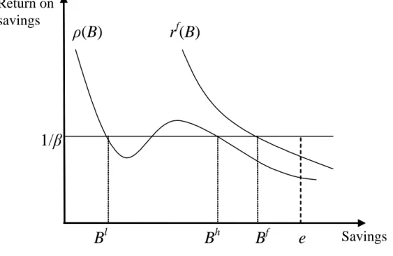
Substituting (8) into (7), we can see that lenders date-1 consumption is e B, while (expected) date-2 consumption is Brf_{(B). Given lenders’ utility function (eq. (2))}

and our assumption of high initial endowment (inequality (3)), lenders increase sav-ings up to the point where rf_{(B) = 1= (see …gure 1). From eqs. (8) and (9), the}

fundamental values of the risky asset and aggregate savings are uniquely determined and given by:

Pf = Rh (10)

Bf = f0 1(1= ) + Rh (11) In other words, lenders’risk neutrality imply that in the fundamental equilibrium asset prices, Pf_{, are equal to the discounted expected dividend stream, R}h_{; while}

capital investment, X_Sf;settles at the point where its rate of return is equal to lenders’ rate of time preference, f0 1_{(1= ). Comparing eqs. (5) and (10) indicates that assets}

are potentially mispriced in the intermediated equilibrium, since the di¤erence P Pf

may be di¤erent from zero; The sign and implications of this mispricing are analysed in Sec. 3.2 below.

3

Multiple lending equilibria

3.1

Expected loan return

Given our assumed utility function (eq. (2)), individual lending decisions simply de-pend on the gross expected return on loans to portfolio investors as compared with the gross rate of time preference. Thus, we must start by analysing the way the expected loan rate, ; varies depending on the amount of aggregate lending, B.

When investors do not default on loans, which occurs with probability , they repay lenders at the contracted rate r (B). When they do default, lenders gather the residual value of investors’ portfolio, f0(XS) XS = r (B) (B P ) : The (expected)

total amount repaid by investors to lenders is thus:

Figure 1: Intermediated vs. fundamental equilibria

ρ(B)

1/β

e

B

B

B

Return on

savings

Savings

r

(B)

which implies that the ex ante unit loan return, as a function of total loans, is: (B) = r (B) (1 ) R

h

B (12)

Note from eqs. (6), (9) and (12) that the probability that investors go bust at date 2, 1 , indexes the distance between the fundamental and the intermedated returns on savings, rf _{and . When = 1 the risk shifting problem disapears since}

portfolio investors never default; The intermediated loan return function, (B) ; is then identical to the fundamental return function, rf_{(B) ;so that the intermediated}

equilibrium becomes uniquely determined by eqs. (10) and (11). When < 1; the distance between these two return functions, for a given level of aggregate savings, is easily shown to be:

rf(B) (B) = r

f_f 1 _rf _rf 1_(r)

B ;

which is positive since xf0 1_{(x) decreases with x (by assumption (1)) and r > r}f

of this crowding out depends on , the probability of a real crisis at date 2, 1 ; measures both the severity of the risk shifting problem in the economy and the implied distortion in the intermediated return on savings.

To analyse the existence and properties of the intermediated equilibrium(a) when < 1, one must characterise the behaviour of (B) _{as B varies over (0; 1). First,} note that (B) is positive and continuous, and that (_{1) = 0 and (0) = 1:}1

Although this implies that 0_{(B)must be negative somewhere, the two terms in the}

left-hand side of equation (12) indicate that, over a given interval [B1; B2] (0;1),

changes in (B)following variations in B are of ambiguous sign.

The …rst term of the right-hand side of (12), r (B), is the decreasing interest rate function characterised in Sec. 2.3 above; An increase in B raises the amount invested in the safe asset, XS, which tends to lower the equilibrium interest rate, r = f0(XS) ;

and thus the average return on loans. In contrast, the second term, (1 ) Rh_=B;

increases with B; This latter e¤ect re‡ects the impact of the total amount of loan on the average riskiness of loans as the composition of the optimal portfolio varies with B. To see this, solve eq. (6) for Rh _{and substitute the resulting expression into (12)}

to obtain:

(B) = r (B) + (1 )XS

B (13)

In other words, the e¤ect of aggregate lending on the loan return is a composition of its e¤ect on the equilibrium interest rate, r (B), and on the share of safe assets in investors’portfolio, XS=B. Now, use eq. (6) again to write the relation between safe

asset investment, XS; and aggregate lending, B, as follows:

B = XS+ Rh=f0(XS) (14)

From eq. (14) and assumption (1) about the concavity of f (:), it is easy to check that an increase in B raises both the quantity of safe assets, XS, and the share of

safe asset investment in investors’portfolio, XS=B. In other words, even though an

increase in B lowers r and thus raises asset prices, Rh_{=r, the relative size of risky}

asset investment, P=B = 1 XS=B; tends to decrease as B increases. This in turn

limits the loss to lenders in case of investor’s default and increases the ex ante return on loans.

Given these two e¤ects at work, the crucial question is, Are there intervals of B over which (B)may be increasing? Taking the derivative of (12) with respect to B,

1_{That (0) = 1 can be seen by using eq. (13) and noting that r (0) = 1 and X}

this is the case if there are intervals of B over which

r0(B) B2 < (1 ) Rh (15) When < 1 condition (15) may be satis…ed if r0_{(B) (> 0) is small enough for}

some values of B, that is, if the equilibrium interest rate is not very responsive to changes in the implied level of safe asset investment, XS. This in turn is true if

f (XS) is ‘‡at enough’ for the relevant range of XS, so that r = f0(XS) responds

little to changes in XS. Using eq. (6), together with the facts that r0(B) = 1=B0(r)

and @f0 1_{(r) =@r = 1=f}00_(X

S), the left-hand side of (15) can be written as follows:

r0(B) B2 = R

h_{+ X}

Sf0(XS) 2

Rh_{+ f}0_(XS)2_{= f}00_(XS)

For XS 2 [X1; X2], which occurs when B 2 X1 + Rh=f0(X1) ; X2+ Rh=f0(X2) ,

r0_{(B) B}2 _{can be made smaller and smaller by decreasing the curvature of f (:) over}

[X1; X2]; In this case f0(XS) is bounded above and below, f00(XS) can be made

arbitrarily small, making r0_{(B) B}2 _{as small as necessary for (15) to hold (provided}

6= 1). Importantly, the larger 1 (i.e., the more severe the risk shifting problem), the more likely (15) is satis…ed, for a given interest rate function, r (B).

Since there may be several intervals of B over which inequality (15) is satis…ed,

0_{(B) potentially changes signs many times as B increases. In the remainder of the}

paper, we shall focus on a particularly simple case of non-monotonicity by assuming that (B) has a single increasing interval, as is depicted in …gure 1 (all our results are easily generalised to the case of multiple increasing intervals). To give a simple example of a class of production technologies generating this property, Appendix A shows that so looks the loan return function if f (x) is isoelastic, where (x) in inequality (1) is a constant that is close enough to zero (formally, (B) has exactly one increasing interval if < (1 p ) =2, none otherwise).

3.2

Loan market equilibrium

The possibility that the expected loan return be an increasing function of the total quantity of loans is an example of ‘strategic complementarity’(in the sense of Cooper and John (1988)) in lending decisions, since the choice by other lenders to increase savings may then lead any individual lenders to vary savings in the same direction. Lenders utility function (eq. (2)) imply that they increase savings as long as (B) >

1= , but decrease savings whenever (B) < 1= ; All equilibria must thus satisfy (B) = 1= . We focus on symmetric Nash equilibria, where consumption/savings plans are identical across lenders and no lender …nds it worthwhile to individually alter his own plan. Then, our normalisation of a unit mass of lenders implies that individual and aggregate quantities coincide in equilibrium.

Multiple intermediated equilibria. Figure 1 below shows how multiple crossings be-tween the (B)-curve and the 1= -line, when they occur, give rise to multiple equilib-ria (this phenomenon is robust since there are in…nitely many production functions, f (:) and associated gross rates of time preference, 1= ; that generate such multiple crossings). Bl _{and B}h _{represent two stable levels of aggregate lending, i.e., where a}

symmetric marginal move away from equilibrium by all lenders alters the loan return in a way that favors the restoration of the equilibrium. The value of B where the (B)-curve crosses the 1= -line from below is not stable and will not be discussed any further (starting from there, an arbitrarily small increase (decrease) in B tends to increase (decrease) (B), triggering a further move away from equilibrium). In both stable equilibria the ex ante return on loans is 1= , and lenders date 1 and (expected) date-2 consumption levels are e Bj _{(j = l or h) and (B) B}j _{= B}j_{= ,}

respectively.

Recall from the previous Section that an increase in B lowers marginal productiv-ity but raises the average riskiness of investors’portfolio. The low-lending equilibrium is thus characterised by a high safe return but a high share of risky assets in investors’ portfolio, while the high-lending equilibrium has a low safe return but a safer average portfolio. Finally, notice that even though both equilibria yield the same ex ante return on loans, 1= , they are always associated with di¤erent levels of interest rates, asset prices and (expected) date-2 output. Indeed, eq. (6) and the fact that Bh _{> B}l

implies that r Bh _{< r B}l _{and X}h

S > XSl, where X j

S; j = l; h denotes the level

of safe asset investment when Bj _{is selected. Then calling P}j _{the asset’s price and}

E ( Y_{j j) expected date-2 output (in the sense of the total quantity of goods available} for agents’consumption) when total lending is Bj_{, we have:}

Ph = Rh=r Bh > Pl = Rh=r Bl

E ( Y_{j h) = f XS}h + Rh > E ( Y_{j l) = f XS}l + Rh

In other words, the selection of the equilibrium with low lending raises the interest rate, depresses asset prices, and lowers productive investment and future output, with

respect to the equilibrium with high lending. (More generally, there may be more than two stable equilibra if (B) has more than one increasing interval, but their properties are similar to the 2-equilibrium case, i.e., the higher B, the lower r(B), the higher P , and the higher XS and E (Y )).

Comparision with the fundamental equilibrium. How do the intermediated levels of lending and asset prices just described compare with the fundamental ones, Bf_{; P}f _;

computed in Sec. 2.4? Appendix B proves the following inequalities:

Pj > Pf; j = l; h (16) Bj < Bf; j = l; h (17) Equation (16) indicates that assets are overpriced in both intermediated equi-libria, i.e., these are associated with a positive bubble in asset prices. This is an immediate consequence of the fact that investors, who are protected against a bad realisation of the asset payo¤ by the use of simple debt contracts, bid up the as-set and overinvest in it (with respect to the fundamental equilibrium). The reason why savings are lower in the intermediated equilibrium than in the fundamental one (eq. (17)) naturally follows; Excess risky asset investment by portfolio investors im-plies that, for any given level of savings B, the intermediated return, (B), is lower than the fundamental one, rf(B) (see our analysis in Sec. 3.1). Lenders must thus ration credit in the intermediated equilibrium (with respect to the fundamental one) up to the point where the intermediated ex ante return, (B) ; is back to the funda-mental one, i.e., the gross rate of time preference 1= (see …gure 1 again). Notice, as a consequence of this analysis, that a ‘double crowding out’is in fact at work on XS in

the intermediated equilibrium. First, for a given level of aggregate savings B, bubbly asset prices crowd out safe asset investment, XS, and raise the equilibrium interest

rate, r = f0(XS) (see Sec. 2.4). Second, lenders’ optimal reaction to the resulting

price distortion is to reduce savings, B, which lowers XS (and raises r) even further.

Welfare. The presence of multiple stable Nash equilibria in the loan market raises the question of their welfare properties, and in particular that of whether they can be Pareto-ranked. Because our economy is one with heterogenous agents, analysing this issue requires computing the ex ante welfare of all classes of agents in each intermediated equilibrium.

First, we know from Sec. 2.3 above that investors’competition for the risky asset implies that they consume zero whether the asset payo¤ turns out well or badly; Their

ex ante welfare is thus zero in both intermediated equilibria. Second, lenders’date-1 consumption is e Bj_{; j = l; h, while their expected date-2 consumption is B}j _(Bj_).

Since (Bj_{) = 1= , j = l; h, lenders’ex ante utility is simply e B}j_{+ B}j _(Bj_{) = e}

in both equilibria. Third, initial asset holders’consumption and welfare at date 1 is the paiment made to them by investors against the risky asset, i.e., the asset price Pj_;

Since Ph _{> P}l_{, they strictly prefer the high-lending equilibrium to the low-lending}

one. Finally, entrepreneurs’ consumption and ex ante utility from borrowing XS

units of goods and investing them in the production technology is f (XS) XSf0(XS),

which is increasing in XS. Since XSh > XSl, entrepreneurs also prefer the high-lending

equilibrium to the low-lending one.

That the high-lending equilibrium Pareto-dominates the low-lending one is not surprising. In the low lending equilibrium aggregate savings are the farthest away from the fundamental equilibrium, the crowding out of capital investment by in‡ated asset prices is the most severe, and so is the resulting output loss at date 2. Now, both investors and lenders are ultimately indi¤erent between which equilibrium prevail; Investors because their competition for the risky asset prevents them from extracting any surplus from their exclusive access to it, and lenders because in equilibrium they earn the same ex ante return whether aggregate lending is high or low. Thus, the welfare loss associated with the choice of the low-lending equilibrium at date 1 must be borne by the two other classes of agents; Entrepreneurs su¤er from the fact that date-2 output is low (because date-1 capital investment is), while initial asset holders su¤er from the fact that asset prices are low (because the bond rate is high).

The strict welfare ranking between the two intermediated equilibria implies that a ‘coordination failure’occurs if agents coordinate on the equilibrium with low lending rather than that with high lending2_{. We know analyse the implications of this possible}

coordination failure in lending decisions in a three-period model where the low lending equilibrium is stochastically selected at the intermediate date.

2_{For similar reasons, in the generalised model with n > 2 lending equilibria, aggregate welfare is}

4

Self-ful…lling crises

4.1

A three-date model

The previous section has shown that the risk shifting problem that arises under market segmentation may lead, under endogenous lending, to the existence of multiple equilibria with di¤erent levels of aggregate lending, interest rates, and asset prices. We now expand the time span of the model to demonstrate the possibility of a self-ful…lling …nancial crisis associated with the selection of the low-lending equilibrium at date 1. Besides o¤ering a stochastic version of the multiple equilibria model, our model of self-ful…lling crisis also has new welfare implications. In particular, it predicts that lenders are also hurt by the crisis because it a¤ects their total wealth, and thus their discounted consumption and utility ‡ows, negatively.

The model has now three date, 0, 1 and 2. Lenders live for 3 periods, and face overlapping generations of two period-lived investors and entrepreneurs entering the economy at dates 0 and 1. In the following we shall refer to ‘date-t investors (entrepreneurs)’ as the investors (entrepreneurs) who enter the economy at date t, t = 0; 1, and leave it at date t + 1. The risky asset is now assumed to be three period lived –it is sold by the one period-lived initial asset holders at date 0 and delivers its …nal payo¤, R, at date 2. The safe asset is two-period lived as before, with x units of assets invested by entrepreneurs at date t, t = 0; 1, yielding f (x) units of good at date t + 1. We assume that f () is ‡at enough over one range of x so that the loan return function at date 1, (B), has exactly one increasing interval just as in the two-period model (here again the model can easily be generalised to the stochastic selection of one lending equilibrium amongst more than two, but we focus on this simple case for sake of expositional clarity).

Lenders receive the endowment e at date 1 as before (where e satis…es condition (3)), and they now also receive e0 > 0 units of good at date 0. They derive utility

from consuming at dates 1 and 2, with a utility function identical to that of the 2-period model (eq. (2)). Because lenders’derive no utility from date-0 consumption, they entrust date-0 investors with their entire endowment from date 0 to date 1 since the gross, expected loan return at date 0 is always positive. As will become clear shortly, this simple speci…cation for lenders’ savings from date 0 to date 1 implies that the equilibrium price of the asset at date 0 is uniquely determined.

the intermediate date of the three-date model will display exactly the same two possible levels of equilibrium lending than the initial date of the two-period model, as we argue below. We can then straightforwardly work backwards equilibrium prices and quantities at date 0, given the possible equilibrium outcomes at date 1 and the likelihood that they actually occur.

We construct equilibria with self-ful…lling crises by randomising over the two pos-sible lending equilibria of the two-date model. To do this, assume that at date 1 high lending is selected with probability p 2 (0; 1), so that a ‘sunspot’causes lending and asset prices to drop down to low levels with probability 1 p. With this speci…cation for extraneous uncertainty about which level of aggregate lending will prevail at date 1, the three-date model potentially has a continuum of stochastic equlibria indexed by the probability of a market crash, 1 p. Since the asset price at date 1 is the asset payo¤ for date-0 investors, this extraneous uncertainty about asset prices creates a risk-shifting problem at date 0 similar to that created at date 1 by intrinsic uncer-tainty about the terminal payo¤ of the asset. This causes the asset to be bid up at date 0, with the possibility that a self-ful…lling crisis occurs at the intermediate date if the low-lending equilibrium is selected.

4.2

Market equilibrium at date 0

Our assumptions made so far ensure that the date-1 equilibria that may prevail in the three-date model are identical to those of the two-date model characterised in Sec. 3.2 above. In particular, our simple speci…cation for lenders’utility imply that, provided the solutions to lenders’ problem are interior (which is guaranteed by assumption (3)), both possible lending levels at date 1, Bl _{and B}h_{, do not depend on lenders}

income at date 1 (this can be checked by varying e in …gure 1 whilst maintaining e > Bf_{). This in turn implies that, within the three-date model, any additional}

income stemming from date-0 investment is consumed at date 1 and does not alter the possible equilibrium lending levels Bj_{, j = l; h, and associated asset prices and}

bond rates, (Pj_{, r(B}j_{)), computed for the two-date model.}

Calling (P0, r0) the equilibrium price vector at date 0, and (X0S; X0R) the portfolio

of date-0 investors, their net payo¤ at date 1 is:

sup [r0X0S+ P X0R r0(X0S + P0X0R) ; 0] = sup [X0R(P r0P0) ; 0] ;

variable taking on the value Ph _{with probability p (i.e., B}h _{is selected), and P}l

otherwise (Bl _{is selected). In the equilibria that we are considering, date-0 investors}

default on loans when the asset price at date 1 is Pl_{, but do not default when it is}

Ph_{. Their payo¤ is thus X}

R Ph r0P0 0 with probability p and 0 otherwise.

Given limited liability and extraneous uncertainty about asset prices at date 1, the consumption of date-0 investors is:

pXR Ph r0P0 (18)

Date-0 investors choose XR that maximises (18), while any potential solution to

their decision problem must be such that they do not default on loans if the asset price at date 1 is Ph_{, but do default if it is P}l_{, i.e.,}

Ph r0P0 0 (19)

Pl r0P0 < 0 (20)

Asset prices. Given (18), the demand for risky assets by date-0 investors is in…nite (zero) if Ph r0P0 > 0 (< 0) :Market clearing thus requires that the equilibrium price

of the asset at date 0 be such that Ph r0P0 = 0, i.e.,

P0 = Ph=r0; (21)

which satis…es inequalities (19) and (20). Here again the interpretation of this equi-librium price is straightforward. The perfect competition for the risky asset by date-0 investors implies that the asset’s price must be such that they make zero expected pro…t. Because they make zero pro…t when the realisation of the asset payo¤ is Pl (i.e., when they default), they must also earn zero even when it is Ph; This is exactly what the equilibrium price Ph=r0 ensures. Note, as a consequence, that the

equilib-rium price at date 0 does not depend on the probability of a crisis, 1 p; Because date-0 investors are protected against a bad shock to the value of their portfolio by the use of debt contracts, they simply disregard the lower end of the payo¤ distribution altogether (i.e., the payo¤ Pl with probability 1 p).

Since lenders do not value date-0 consumption, aggregate lending from date 0 to date 1 is e0 provided the expected loan return at date 0 is positive (this is always

the case since, even in case of investors’default, lenders get some positive repayment, i.e., the value of the liquidated portfolio). In equilibrium we have X0R = 1 and

r0 = f0(e0 P0). Thus, r0 is uniquely determined by the following equation:

where Ph _{= R}h_{=r B}h _{is independent of e}

0, due to the interiority of Bh allowed by

assumption (3). Equations (21) and (22) then fully characterise the intermediated price vector at date 0, (P0; r0), given e0 and Ph.

Asset bubble and crowding out. Finally, we show that the risk-shifting problem due to date-1 extraneous uncertaintly and limited liability of date-0 investors implies that assets are also overvalued at date 0, and that they crowd out real investment then, X0S. To see this, …rst call (P0f; r

f

0) the vector of fundamental prices at date 0, and note

that the date-1, fundamental asset payo¤ in the 3-period model is the fundamental asset price of the 2-period model, Pf _{= R}h _{(see eq. (10)). Application of the usual}

no-arbitrage condition then implies that the fundamental value of the asset at date 0 is: P₀f = Pf=r₀f (23) Since rf0 = f0(e0 P f 0)in equilibrium, r f

0 is uniquely determined by the equation:

f0 1(rf₀) + Pf=r₀f = e0 (24)

Using (22) and (24), the date-0 bubble in asset prices is given by: P0 P0f = f0 1(r

f

0) f0 1(r0)

From equations (22) and (24), and the fact that Ph _{> P}f_{, it is easily seen that}

r0 > rf0. Since f0 1(:)is decreasing, there is a positive asset price bubble at date 0.

Looking at the crowding out e¤ect of this bubble, note that e0 being exogenously

given, the amount of crowding out that takes place in the intermediated equilibrium is simply X_0Sf X0S = P0 P0f > 0: The implied lower level of capital investment at

date 0 in turn lowers date-1 output, f (X0S), in the same way as date-2 (expected)

output, f (XS) + Rh; was lowered by bubbly asset prices at date 1 (see Sec. 3.2

5

The welfare cost of crises

5.1

The wealth e¤ect of crises

The analysis presented in Section 4 consisted of extending the deterministic, two-period framework with multiple equilibria to a stochastic, three-two-period one charac-terised by a continuum of equilibria indexed by the crisis probability, 1 p. In doing so we paved the way for an analysis of the dimension in which these two models really di¤er, i.e., their welfare implications. In the two period model, lenders’wealth at the beginning of date 1 was exogenous (equal to e). Combined with the facts that lenders’intertemporal elasticity of substitution between date 1 and date 0 is in…nite, and that the ex ante loan rate between dates 1 and 2 is equal to the rate of time preference, this meant that lenders ex ante utility was itself equal to e, regardless of which equilibrium actually prevailed.

This is no longer the case in the three period model, because lenders’wealth at date 1 now also depends on the value of their date-0 investment, which is contigent on the sunspot state at date 1. More speci…cally, we now show that the stochastic selection of the low lending equilibrium depletes lenders …nancial wealth of forces them to cut their intertemporal consumption ‡ow. In other words, the three-period model takes into account the wealth e¤ect of …nancial crises on lenders’ possible consumption plans and implied utility.

To see why lenders’ wealth at date 1 is contingent on whether a crisis occurs at date 1 or not, compute the way it is a¤ected by the possible default of date-0 investors. When these investors do not default, they owe lenders the capitalised value of outstanding debt at date 1, r0e0. As lenders receive an endowment e at date

1, their date-1 wealth if no crisis occurs is simply Wh = e + r0e0. When investors

do default, on the contrary, lenders wealth at date 1 is their date-1 endowment, e, plus the residual value of date-0 investors’ portfolio, i.e, Wl = e + r0X0S + X0RPl.

Using the fact that in equilibrium we have X0S = e0 P0, X0R = 1, and P0 = Ph=r0;

we …nd that lenders’wealth, Wj; j = l; h, conditional on the fact that a crisis occurs (j = l) or not (j = h), is given by:

Wl = e + r0X0S+ Pl (25)

Wh = e + r0X0S+ Ph (26)

Obviously, the total quantity of goods at date 1 is the same accros equilibria, be-cause initial capital investment, X0S, is uniquely determined. This quantity amounts

to lenders’ date-1 endowment, e, plus total production, f (X0S) ; the latter being

shared between date-0 entrepreneurs, who get f (X0S) r0X0S in competitive

equi-librium, and lenders, who get r0X0S (recall that date-0 investors always consume

zero, as was shown in Sec. 4.2 above).3

From condition (3) and inequality (16), we have Bj _{< B}f _{< W}j_{, j = l; h,}

implying that both possible levels of wealth give rise to interior solutions for con-sumption/savings plans at date 1 where (Bj_{) = 1= . If a crisis occurs at date 1,}

then lenders’wealth and savings are Wl _{and B}l_{; respectively, while their date-1 and}

(expected) date-2 consumption levels are Wl _Bl _{and B}l_{= , respectively; It follows}

that their discounted utility ‡ow from date 1 on is simply Wl_{. Similarly, if a}

cri-sis does not occur at date 1, then lenders date-1 and date-2 consumption levels are Wh _Bh _{and B}h_{= , respectively, yielding a discounted utility from date 1 on of W}h_.

Weighing these possible outcomes at date 1 with the probabilities that they occur, we …nd that lenders ex ante utility (i.e., from the point of view of date 0) depends on the probability of a crisis, 1 p, as follows:

EUL(p) = pWh+ (1 p) Wl

= e + r0X0S+ pPh + (1 p) Pl;

which is decreasing in 1 p, since Ph _{> P}l _{and e + r}

0X0S; Pl and Ph do not depend

on p. Note that it is the selection of the low lending equilibrium itself that triggers the crisis which lowers lenders’wealth and discounted utility. Thus, the utility loss incurred by lenders when a crisis occurs is akin to a pure coordination failure in consumption/savings decisions –rather than an exogenously assumed desctruction of value associated with the early liquidation of the long asset, as is typically assumed in liquidity-based theories of …nancial crises (e.g., Diamond and Dybvig (1983), Allen and Gale (2000)).

3_{There are two equivalent ways of characterising lenders’budget set at date 1. Looking at wealth,}

total wealth Wj _{is assigned to date-1 consumption and date-1 lending, so that, using eq. (25)-(26),}

e + r0X0S+ Pj = cj1+ Bj; j = l; h

Looking at the total quantity of goods that accrues to lenders at date 1, these are ultimately shared between date-1 consumption, cj₁; and date-1 capital investment, X_Sj, so that:

e + r0X0S= cj1+ X j

S; j = l; h

5.2

Initial asset holders, investors, and entrepreneurs

The previous section has analysed the welfare cost of self-ful…lling …nancial crises from the point of view of lenders. The full welfare analysis of the three-period model, and the potential welfare ranking of the many existing equilibria, requires computing the way the crisis probability, 1 p, a¤ects the consumption of other agents, i.e., initial asset holders, date-0 and date-1 investors, as well as date-0 and date-1 entrepreneurs. Initial asset holder. We showed in Sec. 4.2 that the price of the risky asset at date 0, P0 is uniquely determined and independent of the crisis probability, 1 p. Since

P0 is the consumption of initial asset holders, their welfare does not depend on the

crisis probability.

Investors. From the analysis in Sec. 3.3 we know that date-1 investors get zero pro…t and consumption even when the asset payo¤ is high, due to their competition for the risky assets hedged by the use of debt contracts. The same reasoning applies to date-0 investors, who compete for the asset at date 0 whilst being protected against the risk that the asset payo¤ turns out to be Pl at date 1. In other words, the consumption of both generations of investors is always zero, so that their welfare as a whole is not a¤ected by the crisis probability.

Entrepreneurs. We know from Sec. 3.3 that date-1 entrepreneurs’ …nal consump-tion is f (XS) XSf0(XS), which increases with XS. Because XSh > XSl, their

ex ante welfare, from the point of view of date 0, is p f Xh

S XShf0 XSh +

(1 p) f Xl

S XSlf0 XSl , which increases with p. Turning to date-0

entrepre-neurs, their ex ante utility is simply f (X0S) X0Sf0(X0S), where X0S depends only

on e0 (and not on p). Thus entrepreneurs welfare as a whole decreases with the

probability of a crisis, 1 p.

To summarise, neither investors’ nor initial asset holders’ and date-0 entrepre-neurs’welfare is a¤ected by the probability of a self ful…lling crisis at date 1. Lenders are, because the crisis destroys their asset wealth and forces them to choose a lower discounted consumption ‡ow. Date-1 entrepreneurs are for the reason analysed in Sec. 3.2 that low lending at date 1 reduces their date-2 pro…t and consumption. Thus, the lower the probability that a self-ful…lling occurs at date 1, the higher aggregate welfare.

6

Concluding remarks

This paper has o¤ered a simple theory of self-ful…lling …nancial crises based on the excess risk-taking of debt-…nanced portfolio investors. In our model, the interplay between the amount of funds available to investors, the composition of their portfo-lio, and the return that they can o¤er creates a strategic complementarity between lenders’savings decisions, which may in turn give rise to multiple equilibria associ-ated with di¤erent levels of lending and asset prices. Expectations-driven …nancial crises may then occur with positive probability as soon as the intermediate date has (at least) two possible equilibrium levels of lending, and lenders’ coordination on a particular equilibrium follows an extraneous ‘sunspot’. We showed that such crisis where associated with a self-ful…lling credit contraction followed by a market crash, widespread failures of borrowers, and low productive investment and future output.

Besides demonstrating that credit intermediation based on debt contracts is a source of purely endogenous …nancial instability, the model developed above also gives new insights into the potential welfare costs of …nancial crises. In our model, the dramatic reduction in savings associated with the selection of the crisis equilibrium at the intermediate date has two implications. First, it causes a reduction in lenders’ wealth as the total value of their capitalised investment drops down, which lowers their discounted consumption ‡ow from the time of the crisis onwards. Second, the credit contraction associated with the crisis causes a fall in productive investment and output, with the consequence of lowering entrepreneurs’pro…ts and consumption levels. Thus, both savers and …nal producers are hurt by the …nancial crisis, while intermediate investors, whose risk is hedged by the use of simple debt contracts, are left unharmed.

This paper has taken as an uncontroversial empirical fact the widespread use of simple debt contracts in lending arrangements, and has just assumed it in the model. Our current aim is now to analyse the ways it can be endogenised given the underlying informational asymmetry, and to check how the risk-shifting problem is modi…ed under more general debt contracts, e.g., where the contracted loan rate may depend on the amount borrowed. That simple debt contracts are optimal when investment strategies –in addition to asset payo¤s–are hidden to lenders has recently been demonstrated by Povel and Raith (2004). However, it is not yet clear in general how the risk shifting problem is altered by the use of optimally designed securities.

Appendix

A. Shape of the loan return curve when

f (:) is isoelastic

With f (XS) = X 1

S = (1 ) ; 2 (0; 1) being a constant, we have B (r) = r 1= ₊

Rhr 1 (see eq. (6)), which in turn implies: r0(B) = 1

B0_(r) =

1

( 1= ) r 1= 1 _Rh_r 2;

where r = r (B) is the interest rate function characterised in Sec. 2.3. From eq. (12), (B) is increasing (decreasing) when r0(B) + (1 ) Rh=B2 > 0 (< 0), that is, when

1

( 1= ) r 1= 1 _Rh_r 2 +

(1 ) =Rh

(r 1= _{+ R}h_r 1₎2 > 0 (< 0)

De…ning Y r1 1= and rearranging the above inequality, we …nd that (B) is increasing (decreasing) when

(Y ) = Y2 + Y Rh 2 1 + Rh 2< 0 (> 0)

(Y ) _{changes sign over (0; 1) if} (Y ) = 0 has two real roots, including one positive root at least. A necessary condition for this to be the case is that the discriminant of (Y ) = 0 be positive, i.e., the following inequality must hold:

1 + 4 ( 1) > (A1) When (A1) holds, the roots Y1, Y2 of (Y ) = 0 are:

Y1;2 = Rh 2 0 @ 1 2 s 1 2 2 4 1 A

Both roots are positive (negative) if 1 2 > (<) . Combined with (A1), this means that (Y )_{changes over sign over (0; 1) if (and only if):}

< 1 p

2 (A2)

(Y ) _{is negative for Y 2 (Y}1; Y2) ; and positive for Y 2 (0; Y1)[ (Y2;1). Since

Y = r1 1= _{, this means that (Y )is negative for intermediate values of r and positive}

otherwise. Using eq. (6), this in turns implies that, provided (A2) is ful…lled, (B) is strictly increasing for intermediate values of B, and strictly decreasing otherwise. Note that when (A2) does not hold then (Y )is strictly positive, and (B)strictly decreasing, over (0; 1).

B. Proof of inequalities (16) and (17)

Let us start with inequality (16). From eq. (5) and (10), the price di¤erence Pj Pf = Rh(1=r (Bj) ) ; j = l; h;is positive if and only if

r Bj < 1 1 = 1 r Bj (1 ) R

h

Bj ;

where eq. (12) and the fact that (Bj_{) = 1= ; j = l; h, have been used to replace 1=}

by a function of Bj_{. Rearranging the latter inequality, we …nd that a necessary and}

su¢ cient condition for Pj _{> P}f _is

Bjr Bj > Rh

Using eq. (6), this inequality is in turn satis…ed if and only if f0 1(r) + Rh=r r > Rh;

which is always true since rf0 1_{(r) = rX}

S > 0 provided B > 0 (see eq. (14)).

Let us now turn to inequality (17). Since (Bj_{) = 1= in both equilibria, we can}

rearrange eq. (12) to obtain:

Bj = Bjr Bj (1 ) Rh (B1) Comparing eqs. (11) and (B1), we have that Bj _{< B}f_{; j = l; h, if and only if}

Bjr Bj Rh < (1= ) f0 1(1= ) ;

or, using eq. (6) again, if and only if

rf0 1(r) < (1= ) f0 1(1= )

rf0 1(r) decreases with r since f0 1(r) + rf0 10(r) = XS+ f0(XS) =f00(XS) < 0

due to assumption (1). Thus, the latter inequality is satis…ed if and only if r > 1= . Solving (12) for r (Bj) and imposing (Bj) = 1= , the necessary and su¢ cient condition for Bj < Bf becomes

r Bj = 1= + (1 ) Rh=Bj > 1= ;

References

[1] Allen, F. and Gale, D. (2000), ‘Bubbles and Crises’, Economic Journal, vol. 110, pp. 236-55.

[2] Allen, F. and Gale, D. (1998), ‘Optimal …nancial crisis’, Journal of Finance, vol. 53, pp. 1245-84.

[3] Borio, E.V., Kennedy, N. and Prowse, S. D. (1994), ‘Exploring aggregate asset price ‡uctuations across countries: measurement, determinants and monetary policy implications’, BIS Working Paper no 40, April

[4] Chang, R. and Velasco, A. (2000), ‘Banks, debt maturity, and …nancial crises’, Journal of International Economics, vol. 51, pp. 169-194.

[5] Chari, V.V. and Kehoe, P.J. (2003), ‘Hot money’, Journal of Political Economy, vol. 111, pp. 1262-92.

[6] Cooper, R. and John, A. (1988), ‘Coordinating coordination failures in Keyne-sian models’, Quarterly Journal of Economics, vol. 103, pp. 441-63.

[7] Diamond, D.W. and Dybvig, P.H. (1983), ‘Bank runs, deposit insurance, and liquidity’, Journal of Political Economy, vol. 91, pp. 401-19.

[8] Kaminsky, G.L. (1999), ‘Currency and banking crises: The early warnings of distress’, IMF Working Paper 99/178, December.

[9] Kaminsky G.L. and Reinhart, C.M. (1999), ‘The twin crises: The causes of banking and balance-of-payments problems’, American Economic Review, vol. 89, pp. 473-500.

[10] Kaminsky G.L. and Reinhart, C.M. (1998), ‘Financial crises in Asia and Latin America: Then and now’, American Economic Review, vol. 88, pp. 444-448. [11] Obsfeld, M. (1996), ‘Models of currency crises with self-ful…lling features’,

Eu-ropean Economic Review, vol. 40, pp. 1037-47.

[12] Povel, P. and Raith, M. (2004), ‘Optimal debt with unobservable investments’, Rand Journal of Economics, vol. 35, pp. 599-616.

[13] Summers, L.H. (2000), ‘International …nancial crisis: Causes, prevention, and cures’, American Economic Review, 2000, vol. 90, pp.1-16.

[14] Velasco, A. (1996), ‘Fixed exchange rates: credibility, ‡exibility and multiplicity’, European Economic Review, 1996, vol. 40, 1023-1035.