HAL Id: hal-02749732
https://hal.archives-ouvertes.fr/hal-02749732
Preprint submitted on 3 Jun 2020
HAL is a multi-disciplinary open access
archive for the deposit and dissemination of
sci-entific research documents, whether they are
pub-lished or not. The documents may come from
teaching and research institutions in France or
abroad, or from public or private research centers.
L’archive ouverte pluridisciplinaire HAL, est
destinée au dépôt et à la diffusion de documents
scientifiques de niveau recherche, publiés ou non,
émanant des établissements d’enseignement et de
recherche français ou étrangers, des laboratoires
publics ou privés.
A robust p-Center Problem under Pressure to locate
Shelters in Wildfire Context
Marc Demange, Virginie Gabrel, Marcel Haddad, Cecile Murat
To cite this version:
Marc Demange, Virginie Gabrel, Marcel Haddad, Cecile Murat. A robust p-Center Problem under
Pressure to locate Shelters in Wildfire Context. 2020. �hal-02749732�
(will be inserted by the editor)
A robust p-Center Problem under Pressure to locate Shelters
in Wildfire Context
Marc Demange · Virginie Gabrel · Marcel A. Haddad · Cécile Murat
Received: date / Accepted: date
Abstract The location of shelters in different areas threatened by wildfires is one of the possible ways to reduce fatalities in a context of an increasing number of catastrophic and severe wildfires. These shelters will enable the population in the area to be protected in case of fire outbreaks. The subject of our study is to determine the best place for shelters in a given territory. The territory, divided into zones, is represented by a graph in which eachzone corresponds to a node and two nodes are linked by an edge if it is feasible to go directly from one zone to the other. The problem is to locate p shelters on nodes so that the maximum distance of any node to its nearest shelter is minimized. When the uncertainty of fire outbreaks is not considered, this problem corresponds to the well-known p-Center problem on a graph. In this article, the uncertainty of fire outbreaks is introduced taking into account a finite set of fire scenarios. A scenario defines a fire outbreak on a single zone with the main consequence of modifying evacuation paths. Several evacuation paths may become impracticable and the ensuing evacuation decisions made under pressure may no longer be rational. In this context, the new issue under consideration is to place p shelters on a graph so that the maximum evacuation distance of any node to its nearest shelter in any scenario is minimized. We refer to this problem as the Robust p-Center problem under Pressure. After proving the NP-hardness of this problem on subgraphs of grids, we propose a first formulation based on 0-1 Linear Programming. For real size instances, the sizes of the 0-1 Linear Programs are huge and we propose a decomposition scheme to solve them exactly. Experimental results outline the efficiency of our approach.
V. Gabrel · M. A. Haddad · C. Murat
Université Paris-Dauphine, PSL Research University, CNRS, LAMSADE, 75016 Paris, France, E-mail: virginie.gabrel,marcel.haddad,[email protected]
M. Demange · M. A. Haddad
School of Science RMIT University, Melbourne, Vic., Australia, E-mail: [email protected]
Work supported by the European Union’s Horizon 2020 research and innovation programme under the Marie Skłodowska-Curie grant agreement No 691161
1 Introduction
In the prevention phase of wildfires, an important issue is to determine the location of fire proof shelters in a given area. The problem is basically to locate p shelters minimizing the maximum distance people have to cover in order to reach one of these shelters in case of fire. From an Operations Research perspective, the problem of locating p centers (warehouses, shelters . . . ) has been extensively studied [?]. In particular, mathematical programming ap-proaches enable to determine optimal solutions for the classical p-Center problem [?].
In our model, the territory, typically with low density habitat, is represented by an adja-cency graph G = (V, E). Each node corresponds to a zone. Two nodes i and j are linked by an edge if and only if it is feasible to go directly from one zone to the other without pass-ing through another area. We assume this is a symmetric relation, which makes this graph undirected. The zones are defined by geographical and spatial criteria. In particular, natural barriers like a river or a cliff are natural boundaries. Of course the size of the zones vary de-pending on the population density. Typical examples of zones are villages and surrounding suburbs or, in the case of very sparse habitat, a homogeneous area with easy interior cir-culation. We assume that these zones have been defined a priori. Each edge (i, j) is valued with a positive number li j that can be seen as a distance or a travelling time. Since nodes represent zones, possibly large, the distance (or travelling time) between adjacent nodes can be measured between median points in the two related areas or as a maximum distance; this choice has no incidence on the model. If adjacent zones correspond to a fragmentation of a large homogeneous territory without clear natural boundaries, then the related edges are just a discrete model of a continuous reality. In other cases however, edges represent an accurate representation of the real environment. According to our model, shelters must be placed on nodes. Considering a shelter on node i and a zone represented by a node j, the distance dji from j to i is the length of a shortest path from j to i in G. Given a solution defined as a set of p nodes, the evacuation distance of zone j is the shortest distance between j and one of the p shelters. The value of a solution corresponds to the longest evacuation distance of nodes. Thus the p-Center problem is to compute a minimum value solution.
A major difficulty in wildfire management is due to the uncertainty associated with fire outbreaks and spreading. The circumstances which interest us are when a wildfire is expected to spread rapidly and to be of extreme intensity. This phenomenon happens for in-stance, on hot and windy days with dense and very dry vegetation. Furthermore the way how the fire spreads is hard to predict, since it depends on meteorological conditions (drought, heat, winds..) and on the nature of the vegetation. The black Saturday disaster in Victoria, Australia in February 2009 and in particular the tragic events in Marysville, a small town devastated by flames, is a perfect illustration. With climate change, such fires are an in-creasing phenomenon and are the subject of the project GEO-SAFE (http://geosafe. lessonsonfire.eu/) under the European Union’s H2020 research and innovation pro-gram. Our study is part of this project. Under these extreme circumstances, in case of a fire outbreak, the whole population of the area has to be evacuated to shelters and stay there until being rescued. This assumes an efficient early warning system and clear messages to evacuate. In this process, we need to take into account that some routes to shelters may no longer be practicable.
To address this challenge, we define a new version of the p-Center problem considering a set of scenarios. A scenario corresponds to a zone on fire meaning that the zone can no longer be reached. Moreover in the emergency context of wildfires, the evacuation decision
is made under pressure and implies a specific evacuation strategy. The evacuation context involves new distances to reach shelters and the value of a solution is computed as the worst evacuation distance. This leads to a specific robust problem called the Robust p-Center problem under Pressure(RpCP).
This paper is organised as follows: in Section 2, we define RpCP and we compare it to the state of the art. In Section 3, we study the complexity of the problem in specific classes of graphs. In particular we establish the NP-hardness of this problem on subgraphs of grids. In Section 4, we propose a new formulation based on 0-1 Linear Programming. Finally in section 5, a new exact algorithm is defined and extensive experimental results show the tractability of our approach.
2 Robust p-Center problem under pressure
In Subsection 2.1, we define and motivate the problem, while in Subsection 2.2, we underline the differences between solutions of RpCP and the classical p-Center problem. Finally in Subsection 2.3, we compare RpCP to relevant variants in the literature.
2.1 Definition
To model fire hazards, a scenario is associated with a specific fire outbreak in the territory that is represented by a graph G = (V, E) with n nodes. We restrict ourselves to single fire outbreak and consequently, each scenario s corresponds to a single node s on fire. This re-striction is motivated by our primary focus on a relatively short time period after outbreak which assumes an efficient early warning system. In this case everybody can escape to a shelter before the fire spreads to adjacent zones. The operational graph associated with the scenario s, denoted by Gs, is a directed graph obtained from G as follows. All edges (i, j) are replaced by two arcs (i, j) and ( j, i) except the edges (s, v) incident to s: these edges are replaced by a unique arc (s, v). Consequently, in Gs, node s is no longer accessible from another node. In Gs= (V, Es), paths are directed and directed shortest paths from a node x6= s in Gscannot go through s. For all i and j, ds
i jdenotes the length of the directed shortest path from i to j in the graph Gs. By convention, for all j ∈ V \ {s}, we have dsjs= +∞ which means there is no path from j to s.
Given a set of p nodes, solution to the p-Center problem, the evacuation distance of a node j is the shortest distance between j and its nearest shelter. This evacuation distance is not relevant in our context since such shortest path may no longer be practicable because of fire. For this reason, we consider a more realistic model to evaluate the evacuation distances to shelters. This model has been discussed with final users as part of the Geosafe project1 and in particular in dedicated open sessions of GEO-SAFE Wildfire conference, (https: //geosafe.lessonsonfire.eu/fireconference/).
In case of a fire outbreak on node s, we have: 1. for people in zone s, two cases have to be considered.
(a) If a shelter is located in zone s, we assume the following: all the persons present in
1 We would like to thank particularly the Pau Costa Foundation (www.paucostafoundation.org/),
the Fire Organisation of Andalucia (INFOCA, www.juntadeandalucia.es/medioambiente/site/ portalweb/), the Fire Organisation of Corsica (SDIS2B, www.sdis2b.fr) and the Country Fire Authority of Victoria, Australia (CFA,www.cfa.vic.gov.au).
that zone can reach this shelter safely. So the evacuation distance is set to zero. To sup-port this hypothesis, we assume that the shelter location in the zone and the local layout guarantee easy accessibility [?] during the phase after outbreak. It is even reasonable to assume that on and around the shelter, clear signs direct people accurately. However, for people outside the zone, to attempt to reach the shelter could be dangerous. For this reason s is not accessible from other nodes in the operational graph Gs.
(b) If there are no shelters in zone s, we assume that people in this zone will first flee in any other direction to reach an adjacent zone j, they will evacuate to the nearest shelter from j in Gs. Thus, the evacuation distance associated with this zone is the worst out of all the possible adjacent nodes to reach first. Without strong evidence (like a shelter in the zone), people, especially under pressure, may react in very diverse ways: choosing for instance to run in the opposite direction of the fire, or in the opposite direction of the wind or in the most accessible direction. On reaching a safer zone, they are more likely to observe the information provided, as their own decisions have become more rational. To ensure an acceptable level of risk, we must consider the worst case scenario. 2. for people who are not in zone s, for example in zone j 6= s, the evacuation distance
from j to shelter k corresponds to ds
jk in graph G
s, i.e., avoiding node s. As already mentioned, we assume that all people in this territory need to be sheltered. Going to the closest accessible shelter is safe. It is important to remember that fires can be very unpredictable, very fast spreading, and can flare up from embers and at a distance. This examination of evacuation distances renders the problem specific compared to the literature and introduces some additional complexity.
For a given p, a solution C of RpCP corresponds to a set of p nodes where to locate the pshelters. For a given solution C and a given scenario s, the evacuation distance of zone j is denoted by rs
j(C). If a shelter is located on j, rsj(C) = 0 otherwise we have:
rsj(C) = min k∈Cd s jk if j 6= s max v∈N+ Gs(s) {lsv+ min k∈Cd s vk} otherwise (1)
where NG+s(s) is the set of all nodes v such that (s, v) ∈ Es.
Notice that rsj(C) is equal to +∞ if j can’t reach any shelter in Gs. In this case, the solution C is not feasible and consequently instances may occur without feasible solutions (see Subsection 2.2 for further details).
The radius associated with scenario s is defined as rs(C) = maxj∈Vrs
j(C). A given so-lution C corresponds to n radius r1(C), . . . , rn(C) for n different scenarios. In the context of emergency evacuation, the value r(C) of a solution C is obtained by considering the worst (max) radius: r(C) = max{r1(C), . . . , rn(C)}. The problem RpCP is then to determine a solution C∗with the minimum worst value:
r(C∗) = min C r(C) = minC maxs∈V r s(C) = min C maxs∈V maxj∈V r s j(C)
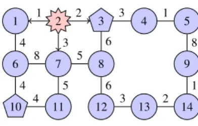
Example 1 Let us consider the operational graph associated with scenario 2 in the Figure 1 where the two arcs (i, j) and ( j, i) are represented by a unique continuous line. The solution C= {3, 10} corresponding to shelters located on nodes 3 and 10 is represented by pentagon nodes. In case of fire on node 2 (scenario 2), the modification of the graph and the evacuation strategy induce:
1 2 3 4 5 6 7 8 9 10 11 12 13 14 1 2 3 4 3 6 1 8 8 4 5 5 6 1 4 3 2
Fig. 1: The operational graph associated with scenario 2 with the solution C = {3, 10}
– The shortest path value from 1 to 3 is no longer 3 but 23, using the shortest path 1, 6, 7, 8, 3. Consequently, the nearest shelter from node 1 is 10 at a distance of 8. Thus the evacuation distance of 1 in scenario 2, is equal to 8 and node 1 is evacuated to node 10.
– To compute the evacuation distance of node 2 in scenario 2, we have to consider three neighbours:
– for neighbour 1, the distance to the nearest shelter 10 is 1 + 8 = 9; – for neighbour 7, the distance to the nearest shelter 10 is 3 + 9 = 12; – for neighbour 3 with a shelter, the distance is 2.
Consequently, r22(C) = 12.
– The radius of the scenario 2 is given by r2(C) = maxj=1,...,14r2j(C) = r 2
13(C) = 15. Finally, the radius of this solution is defined by r(C) = max
s=1,...,14r
s(C) = 35 induced by node 4 in scenario 3.
u t
2.2 Comparison with the p-Center problem and feasibility condition
A solution C ⊂ V for RpCP is feasible if it has a finite evacuation distance for all nodes in all scenarios. In some cases, most of the feasible solutions of the p-Center problem are no longer feasible for RpCP. For example, consider the path G given in Fig 2. When p = 2, any set of 2 nodes is a feasible solution for the 2-Center problem while the only feasible solution for the robust 2-Center problem is the set {1, 5} of the extremity nodes of the path. For all C without node 1 (or equivalently 5), we necessarily have r21(C) = +∞ (since node 1 cannot reach any shelter) and the solution C is not feasible.
1 2 3 4 5
Fig. 2: A path with 5 nodes and shelters on the extremities
We observe that any feasible solution for RpCP must include all nodes of degree 1, called leaf nodes. Consequently, when p is smaller than the number of leaf nodes, RpCP admits no feasible solutions.
Moreover, a solution C ⊂ V for RpCP has a finite evacuation distance for all nodes in all scenarios when, in all subgraphs Gs, there is a path between any node v ∈ Gsand a shelter.
This implies the need for a shelter to be located in any connected components of Gs for all scenarios s. Let us denote ccsthe number of connected components of Gs. When p is smaller than maxs∈Vccs, RpCP admits no feasible solutions.
Even when any solution of the p-Center problem is feasible for RpCP, the relative error of using an optimal solution of the p-Center problem for RpCP can be arbitrarily large, as shown in the following. Consider the instance represented in Figure 3, for M ≥ 1. The opti-mal choice for the 2-Center problem is to locate shelters at nodes 2 and 3, for a radius of 1. The value of this solution in R2CP is M + 3, induced by the evacuation distance of node 1 to shelter 3 in scenario 2. However, if we locate the shelters at node 5 and 6, the worst radius value is 3 induced by scenarios 2, 3, 5 and 6. The relative error of using an optimal solution of the 2-Center problem for R2CP is (M+3)−33 =M3.
1 2 3 4 6 5 1 2 1 1 1 1 2 M
Fig. 3: Comparing the optimal solutions of the 2-Center problem and R2CP
To the best of our knowledge, RpCP including our specific evacuation strategy has never been studied so far. Some variants of the p-Center problem close to our model are proposed in the literature. In the next section, we present some of them and underline the main differ-ences.
2.3 Comparison with the state of the art
The robust version of the p-Center problem is usually defined by introducing uncertainty of edge weights: each weight may vary in an uncertainty set (usually an interval) and the prob-lem is to determine a solution minimizing the worst case or the maximum regret [?,?,?,?]. In [?], authors apply the Bertsimas and Sim approach [?] to model and to solve a p-Center prob-lem with interval associated to edge weights. In these works, weights vary independently one from each other. In our context, this independence hypothesis is not relevant since, if a fire ignites on a node, all weights of the edges incident to this node are modified in the same way. In our context however, uncertainty has to be represented by a set of discrete scenarios. Such approach has already been studied for facility location problems [?,?]. These two pa-pers review the literature on stochastic and robust facility location models. Most deal with scenario-based approaches on generalizations of the p-median facility location problem. For example, in [?], a p-median problem under scenario-based demand uncertainty is consid-ered. In [?], a new robustness measure is introduced and used on a discrete scenario-based approach for the p-median problem. This measure consists in minimizing the expected cost under the constraint that the relative regret is bounded in each scenario. More recently, in [?], authors propose a stochastic evacuation planning model that optimally locates shelters and assigns evacuees to the nearest shelter so as to minimize the expected total evacuation time. The two reviews [?,?] underline that robust p-Center problems are often more difficult
than the related p-median problems. This explains why scenario-based approaches were not considered for the p-Center problem until very recently. To our knowledge, the only paper studying the robust p-Center problem with a scenario approach is [?]. They propose a robust model for a reliable p-Center problem. Each scenario corresponds to a set of disrupted facil-ities and updated demands and costs. Clients are reallocated to the nearest surviving facility. In all these studies, different travel times on the edges are realised for different scenarios. Given a solution C, the radius of node j in scenario s is: mink∈Cdsjk. This distance only corresponds to the case j 6= s in Equation 1 defining the evacuation distance rs
j(C). In the other case ( j = s), the evacuation distance is no longer computed with a min operator over Cbut with a max min since maxv∈N+
Gs(s){lsv+ mink∈Cd s vk} = maxv∈N+ Gs(s)mink∈C{lsv+ d s vk}. This case is due to our specific evacuation strategy that differentiates our problem from the classical scenario-based approach.
In [?], Chaudhuri, Garg and Ravi consider the k-neighbour p-Center problem. It is a generalization of the p-Center problem where, given a number k, we have to place p centers so as to minimize the maximum distance of any non-center node to its kth closest center. They give a 2-approximation algorithm for this problem, and show it is the best possible. However, the evacuation strategy in RpCP does not correspond to an automatic reassign-ment to a kthcenter. For a given solution and for all scenarios s, we do not assign node v to some predetermined kthclosest center in G, because, among other things, we have no guar-antee that the kthclosest center for v in G is accessible in Gs. If we consider graph Gs, while the nodes v ∈ V \ {s} are evacuated to their closest center in Gs, the evacuation strategy of node s depends on its neighbourhood. Thus, there is no simple way to reduce RpCP to the k-neighbour p-Center problem.
In a variant of the p-Center problem for large-scale emergencies considered in [?], the disaster affects a single node s, including any facility (e.g. a shelter) on this node. The differ-ence with our model is twofold. Any facility on an affected node is no longer available but only the population on this node requires evacuation. This model is motivated by different kind of disasters that affect a single node but also by the fact that each node corresponds to a large zone, like an entire city. Our context is really different since all zones must be evacuated in each scenario s and a shelter always secures at least the people from the corre-sponding area.
So, to the best of our knowledge, the RpCP that we introduce with specific evacuation strategy under pressure has never been studied. In the following section, we analyze the complexity of RpCP on different classes of graphs.
3 Complexity
RpCP is clearly polynomial (even thought not tractable in practice) for any constant p; so, in this section, we will consider that p is not fixed and thus, it is part of the input.
For this section, we consider the decision version of RpCP with constant threshold. For any constant k, RpCPktakes as input an integer k and an instance of RpCP; it is to decide whether there is a solution C with radius r(C) ≤ k. This problem is clearly in NP: we consider a polynomial number of scenarios and consequently, for any solution C, checking whether r(C) ≤ k can be done in polynomial time. For each scenario, it requires evaluating the evacuation distances of each node using a minimum path algorithm.
In this paper, we will address k = 1 or 2 and all edges of length 1. For k = 1, we outline a close relation between RpCP1and the problem of deciding whether a graph has a node cover of size p, i.e., a set of p nodes such that each edge of the graph is incident to at least one node of the set (Minimum Node Cover problem). Then, we consider a subclass of bipartite planar graphs, the class of induced subgraphs of a grid called subgrids, that is a realistic class of real instances. RpCP1is polynomially solvable in this class while RpCP2reveals to be NP-complete. We conclude with some comments about the complexity of RpCP.
3.1 RpCP1and the Minimum Node Cover problem
We consider an undirected graph G = (V, E), where all edges are of length 1. The following elementary proposition leads immediately to a first hardness result: Proposition 1 Let G be a graph. The radius of a set of nodes C ⊆ V is at most 1 if and only if C is a node cover that includes all leaf nodes.
Proof Suppose C a set of nodes with r(C) ≤ 1. Since its radius is finite, it should include all leaf nodes. Let u ∈ V \C, then for scenario u (u is on fire) and the set C, we have ru
u(C) = 1, which means that all neighbours of u are in C. Thus, C is a node cover.
Conversely, if C is a node cover including all leaf nodes, we consider a scenario u and a node v such that v /∈ C (in particular v is not a leaf node). If v = u, since v /∈ C, every neighbour of v is in C. If v 6= u and since v is of degree at least 2, v has at least one neighbour in C \ {u}. In both cases, the evacuation distance is 1 and consequently ru(C) = 1. Therefore, r(C) ≤ 1, which completes the proof.
u t In particular, if G has no leaf node, then r(C) is at most 1 if and only if C is a node cover. We deduce immediately:
Corollary 1
1. RpCP1 is NP-complete in all classes of graphs of minimum degree 2 for which the decision version of Minimum Node Cover problem is NP-complete. The problem RpCP is NP-hard in these classes of graphs.
2. RpCP1 is polynomial-time solvable in all classes of graphs of minimum degree 2 for which the decision version of Minimum Node Cover problem is polynomial-time solv-able.
For hereditary classes of graphs H, we can easily use a pre-processing allowing to reduce the Minimum Node Cover problem in this class to the same problem in the subclass of graphs in H without leaf nodes. This leads to the following corollary.
Corollary 2
1. RpCP1is NP-complete in all hereditary classes of graphs for which the decision version of Minimum Node Cover problem is NP-complete. The problem RpCP is NP-hard in these classes of graphs.
2. RpCP1 is polynomial-time solvable in all hereditary classes of graphs for which the decision version of Minimum Node Cover problem is polynomial-time solvable.
The proof is not essential for this paper and consequently, to make the text easier to read, it is detailed in Appendix A.1.
In particular, deciding whether the minimum radius is 1 (RpCP1) is NP-complete on planar graphs of maximum degree 3 since the decision version of Minimum Node Cover is NP-complete on this hereditary class [?]. The case of planar graphs of low degree is particularly relevant for real case applications. Since the graph G represents the adjacency graph of zones in the territory, it is planar and in most cases, each zone has a small number of adjacent zones. In some cases however, the underlying graph has even a simpler structure. A common case is a rectangular grid or a subgraph of a grid (called subgrid) when the territory has some “holes” corresponding to large spaces not likely to burn like a lake, a clearing or even a stone field. Based on these cases, a natural question is the complexity of RpCP in bipartite planar graphs and even in subgrids. In what follows, we answer this question.
3.2 RpCP2in subgrids
The main result of this subsection is Theorem 1 that states the hardness of RpCP2in sub-grids. To make the presentation easier to read and the proof more intuitive, we first propose a weaker result (Proposition 2) stating the hardness of RpCP2in bipartite planar graphs of maximum degree 3. Then, we show how to extend the reduction with a more complex con-struction to prove Theorem 1. This step uses ideas and techniques proposed in [?,?] to prove NP-hardness results in subgrids for a large range of problems known to be hard in planar bipartite graphs with nodes of degree 2 or 3.
Proposition 2 RpCP2is NP-complete in planar bipartite graph with nodes of degree 2 or 3, even if all edges have length 1. RpCP is NP-hard in this case.
Proof We revisit a reduction mentioned in [?] for another problem. The reduction is from the decision version of Minimum Node Cover problem in planar graphs with nodes of degree 2 or 3, known to be NP-complete [?]. Since this Proposition is weaker than Theorem 1, we propose in the main text a sketch of proof and report in Appendix A.2 the proof of the main argument (Claim 1). It is not essential for the paper but helps understanding the proof of Theorem 1.
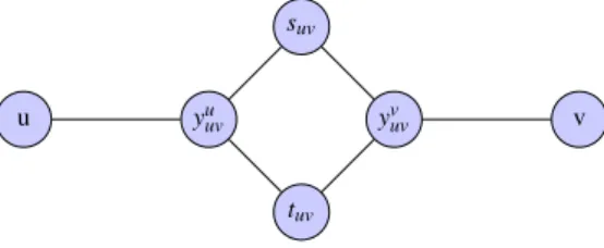
Given a planar graph G = (V, E) with degrees 2 or 3, one builds a bipartite graph G0= (V0, E0) by replacing each edge (u, v) with a gadget Luvas presented in Figure 4. G0has all its nodes of degree 2 or 3.
u yu uv suv yv uv tuv v
Fig. 4: The gadget Luvfor an edge (u, v)
Claim 1 For any t ≤ |V |, G has a node cover of size t if and only if G0has a set C of(t + |E|) nodes with r(C) ≤ 2. Moreover, for each edge (u, v) ∈ E, C has exactly one node in {yu
uv, yvuv} and none in{suv,tuv}.
Proof (of Claim 1) We prove only the necessary condition and prove the sufficient condition in Appendix A.2. Suppose first that G has a node cover U ⊂ V of size t, we will add to it a set UE of nodes to make it the required set of centers. To make the following construction non-ambiguous, we consider an orientation of the graph G. Consider any edge (u, v) oriented from u to v. If u ∈ U , then we add yvuvto UE and if v ∈ U but u /∈ U, then we add yuuvto UE. Then, U ∪UEis a set of (t + |E|) nodes of radius 2 (nodes in V are of degree at least 2).
u t Claim 1 states that the decision version of Minimum Node Cover in planar graphs with nodes of degree 2 or 3 polynomially reduces to RpCP2 in this class of graphs. Since the former problem is NP-complete in this class, so does the latter, which concludes the proof.
u t In what follows we show how we can adapt the proof of Proposition 2 to prove a stronger result. It seemed to us easier to devise directly a reduction from Minimum Node Cover than reducing RpCP2in planar graphs with nodes of degree 2 or 3 to the same problem in a more restrictive class. The proof of Proposition 2 is given only to make this reduction clearer and more intuitive.
Theorem 1 RpCP2is NP-complete in subgrids with nodes of degree 2 or 3, even if all edges have length 1. RpCP is NP-hard in this case.
Proof We already have noted that the problem RpCP2is in NP. For clarity, the reduction is divided in two steps.
Step 1: This step follows general ideas proposed in [?,?] for proving NP-hardness results in subgrids. Given a planar graph G = (V, E) with nodes of degree 2 or 3, we first embed it in a grid of polynomial size using a result of [?]: nodes are mapped to nodes of the grid and edges are mapped to non-crossing paths in the grid. Embedding can be done in polynomial time. For seek of simplicity, for every node u of G, we will denote as well by u the node of the grid it maps to. Using this convention, we consider that the node set of G is contained in the node set of the embedding of G in the grid. Thus, any edge (u, v) of G is replaced by a path of length `uvbetween u and v in the embedding for some positive integer `uv. The resulting graph is not a subgrid but only a partial subgraph of the grid. The next step will make it a subgrid with, in addition, the required properties to ensure the validity of the reduction.
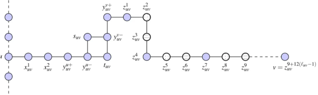
Step 2: The main idea is inspired from the reduction seen in Proposition 2, where a 4-cycle was inserted on each edge of the original graph (gadget of Figure 4). After embedding the graph in a grid, an edge (u, v) of the original graph is a path of length `uv and the idea is to insert on this path a 4-cycle like in the previous reduction. The only technical difficulty is to manage the length of the paths between u, v and this 4-cycle to ensure the reduction will work. To this aim, we use the gadget Huvrepresented in Figure 5 with nodes x1uv, x2
uv, yu+uv, yu−uv, suv,tuv, yv+uv, yv−uv and ziuv, i = 1, . . . , 9. It can be seen as a gadget similar to Figure 4 (nodes yu+uv, yu−uv, suv,tuv, yv+uv, yv−uv) with two paths of 3 and 9 edges attached to yu+uv and yv+uv, respectively. Note that this gadget can replace a section of 12 consecutive horizontal edges and similarly, a sequence of 12 vertical edges can be replaced with the same gadget rotated byπ
2. To this purpose, the next step after step 1 is to subdivide every edge in 12 edges by inserting 11 new nodes. This has few advantages: it produces another embedding of the
original graph in a grid that ensures that every path Puvin the grid associated with an edge (u, v) of the original graph has now 12`uvedges and with its 12 first edges from u (or from v) either all horizontal or all vertical. In addition, such an expansion gives enough space to ensure we can insert gadgets Huvwhile guaranteeing the resulting graph to be a subgrid. The strategy is to insert Huvby replacing the 12 first edges on one side of Puv. Since it is non symmetric, we will use an orientation of the original graph G. Starting from the graph obtained at step 1, the second step is summarized below and will conclude the reduction:
– Subdivide every edge in 12 edges by inserting 11 new nodes. The resulting graph, G0 is a subgrid obtained from G by replacing any edge (u, v) of E with a path Puvof 12`uv edges.
– Select an orientation of each edge of G.
– For an edge (u, v) oriented from u to v, replace the 12 first edges of Puv, starting from u, with the gadget Huvrepresented in Figure 5 if the 12 replaced edges are horizontal or with the same gadget rotated by π
2 if they are all vertical. – The resulting graph is denoted by eG
u x1 uv x2uv yu+uv yu−uv tuv z5uv z6uv z7uv z8uv z9uv suv yv−uv yv+uv z1uv z2 uv z3 uv z4 uv v= z9+12(`uv−1) uv
Fig. 5: The Gadget Huvfor the edge (u, v) oriented from u to v (continuous lines are used for Huv’s edges while dashed lines correspond to edges outside Huv)
Note that for any edge (u, v) of G oriented from u to v, there is a path of length 12(`uv−1) in eGfrom the node z9
uvand v. In particular, if `uv= 1, then z9uv= v. Else, the nodes of this path are denoted by z10uv, . . . , v = z
9+12(`uv−1)
uv . We then denote by Huv0 the subgraph obtained by adding to Huvthe path from z9
uv to v. If `uv= 1, then Huv0 = Huv. The graph Huv0 has 6 + 12`uvnodes including u and v. The graph eGis obtained from G by replacing each edge (u, v) oriented from u to v with Huv0 . It is an induced subgrid since for every node x of Huv\ {u, v} and for every node y of Hu0v0\ {u0, v0} with (u, v) 6= (u0, v0), (x, y) is not an edge in the grid. In addition, nodes in V have the same degree in eGthan in G and all other nodes in eG have degree 2 or 3. So, eG has |V | + 4|E| + 12L nodes, all of degree 2 or 3, where L= ∑
(u,v)∈E (`uv).
This concludes the construction that can be performed in polynomial time. To conclude the proof of Theorem 1, we need to show that the Minimum Node Cover in the graph G reduces to RpCP2in the graph eG. For this, we establish two claims. Claim 2 is a technical result proved in Appendix A.3. It is used to prove Claim 3 that immediately concludes the proof.
Claim 2 Let C be a set of nodes of radius at most 2, then for every edge (u, v) of G oriented from u to v, the following holds:
1. C includes at least one node from{suv,tuv, yu−uv, yv−uv}
2. C includes at least two nodes from{suv,tuv, yu−uv, yv−uv, yu+uv, yv+uv} The proof is given in Appendix A.3.
We are now ready to establish Claim 3. The proof requires to define, for an edge (u, v) ∈ E of G oriented from u to v, two disjoint sets of nodes of Huv0 :
Denote Cv+
uv = {z3iuv, i = 1, . . . , 2 + 4(`uv− 1)} (last node is z
6+12(`uv−1)
uv ); Denote Cuvv−= {z3i−1uv , i = 1, . . . , 3 + 4(`uv− 1)} (last node is z
8+12(`uv−1)
uv , which is linked to v).
Cuvv+ and Cuvv− include, after a first node z i0
uv, every third node along the path zi
uv, i0≤ i ≤ 8 + 12(`uv− 1). Roughly speaking, Cv+
uv (resp. Cuvv−) corresponds to the optimal position of centers along the path from yv−uv to v in Huv0 after deciding to implement a center on node yv+uv (resp. yv−uv). Note that on a path with 3k + 1 nodes, at least k − 1 centers are required in addition to the two extremities to ensure the radius to be at most 2. The only solution using this number of centers is to place centers at the extremities of the path and on every third node in between. We have |Cv+
uv| = 2 + 4(`uv− 1) and |Cv−uv| = |Cuvv+| + 1. In Figure 5, nodes in Cuvv+and Cuvv−are filled with lines and dots respectively.
Claim 3 G = (V, E) has a node cover K of size k = |K| if and only if eG has a set CK of (k + 4|L| + |E|) nodes with r(CK) = 2.
Proof (of Claim 3)
Let us first consider a node cover K of cardinality k in G = (V, E). We complete K in CK in e
Gby adding, for every edge (u, v) ∈ E of G oriented from u to v, 4`uv+ 1 nodes as follows: If u ∈ K, then we add to CKnodes {yu+uv, yv−uv} ∪Cuvv−.
If u /∈ K, then we add to CKnodes {x1
uv, yu−uv, yv+uv} ∪Cv+uv.
Since we add 1 + 4`uvnodes for each edge, we have: |CK| = |K| + 4|L| + |E|. We can check that the radius of CKis at most 2 and it is at least 2 since, in all cases, we have two consecutive nodes in Huvthat are not in CK.
To prove the converse, note first that we need at least 1 + 4`uvnodes of Huv0 \ {u, v} in CK to ensure r(CK) ≤ 2. Actually, if there are three consecutive nodes of degree 2 that are not in CK, then the radius is at least 3. Consequently, even if u and v are in CK, we need at least 4`uvcenters of Huv0 \ {u, v, suv,tuv, yu−uv, yv−uv} to ensure that every three consecutive nodes of degree 2 include at least one center. The best way to do it is to add {yu+uv, yv+uv} ∪ Cv+uv, which makes 4`uv centers. Using Claim 2 (first item), at least one additional node from {suv,tuv, yu−uv, yv−uv} should be added in any set of nodes C satisfying r(C) = 2.
Let us now assume that eGincludes a set of nodes C of radius 2. As we just noted, for every edge (u, v) of G, C includes at least 1 + 4`uvnodes of Huv0 \ {u, v} and thus, C includes in all k + |E| + 4L nodes for some non-negative k. Suppose now that, for an edge (u, v) of G, oriented from u to v, neither u nor v is in C. Since r(C) ≤ 2, we have {x1
uv, x2uv} ∩C 6= /0 and {z8+12(`uv−1)
uv , z7+12(`uv uv−1)} ∩ C 6= /0. Then, since we cannot have three consecutive nodes of degree 2 outside C, |C ∩ {zi
uv, i = 1, . . . , 8 + 12(`uv− 1)}| ≥ 4`uv− 1. Using Claim 2 (second item), at least two nodes from {suv,tuv, yu−uv, yv−uv, yu+uv, yv+uv} should be in C. In all, C has at least 4`uv+ 2 nodes in Huv0 . These nodes can be replaced with {u, yu+
augmenting the cardinality of the set. By repeating this transformation, we obtain a set of nodes C0such that |C0| ≤ k + 4|L| + |E|, where C0∩V is a node cover of size at most k. This completes the proof of Claim 3.
u t Claim 3 states that the decision version of Minimum Node Cover in planar graphs with nodes of degree 2 or 3 polynomially reduces to RpCP2 in this class of graphs. Since the former problem is NP-complete in this class [?], so does the latter. This concludes the proof of Theorem 1.
u t
3.3 Does increasing the radius make the decision problem harder?
Subsection 3.2 gives an example of graph classes for which RpCP2is hard while RpCP1 is polynomially solvable. Meanwhile, Subsection 3.1 outlines classes of graphs for which RpCP1is hard without any evidence about hardness of RpCP2 on these classes. These re-sults make natural the question of the hardness of RpCPkwhen k varies. Is there a reduction allowing to state the hardness of RpCPk+1on a class if RpCPkis known to be hard on this class? In particular, can we conclude results for larger k values for the classes studied here? The following remark gives evidence of graph classes on which RpCP1is hard but RpCP2 is trivial. This justifies that such a reduction from a k to k + 1 does not exist in the general case and consequently, the hardness of RpCPkon a given graph class requires to be studied for any value of k and cannot be deduced, in general, from hardness results dealing with different values of k. This leaves open avenues for future researches with, in particular, the challenge to devise reductions working for different values of k.
Proposition 3 There are graph classes for which RpCP1is NP-complete while all graphs in the class have a solution of radius 2 using only two centers (thus, RpCP2is trivial).
Proof Consider any classC of graphs with all nodes of degree at least 2 and including at least three independent nodes (i.e., not linked by an edge) such that the decision version of Minimum Node Cover problem is NP-complete onC . The condition that at least three independent nodes exist in any graph G = (V, E) of this class is not restrictive since Node Cover can be trivially solved in polynomial time on graphs that do not satisfy this condition. The condition ensures that the size of a minimum node cover is at most |V | − 3 for any graph G= (V, E) ∈C . We build the class C0of all graphs obtained from a graph G ∈C by adding two nodes u0, v0completely linked to all nodes of G. For any graph inC0, a minimum node cover includes u0, v0and a minimum node cover of the graph obtained by removing u0, v0. If u0or v0is not included in the node cover, then all other nodes should be included which, by hypothesis, is larger than the proposed solution. So, the decision version of Minimum Node Cover problem and RpCP1 using Corollary 1 are both NP-complete onC0. Note however that for any graph inC0obtained from G = (V, E) ∈C by adding u0, v0, the set {u0, v0} is a solution of R2CP of radius 2, which completes the proof.
u t In the following section, we propose an integer linear programming (ILP) formulation for RpCP. This model is inspired by the models proposed in [?,?] for the p-Center prob-lem. We generalize this model to take into account different fire scenarios and our
evacu-ation strategy. When handling both robust p-Center problem under pressure and the usual p-Center problem, the latter will be qualified as deterministic, unless no confusion occurs.
4 Integer Linear Programming model for the robust p-Center problem under Pressure
We propose an ILP model with 0-1 variables representing the maximal radius over all the scenarios to be minimized under linear constraints. The starting point of our model is the deterministic p-Center model presented in [?]. We recall this model in the next sub-section.
4.1 Integer Linear Programming model for the deterministic p-Center problem
The deterministic p-Center model presented in [?] is similar to the model proposed by El-loumi, Labbé and Pochet in [?]. In [?], the formulation is based on the observation that the optimal value of the p-Center problem corresponds to one of the distances between two nodes in G. Denote D the finite list of distinct distances between nodes, using the distance of shortest path lengths. Starting with the matrix SP = (di j) of the shortest path lengths be-tween every couple of nodes (with dii= 0 and di j= dji= +∞ if there is no path between i and j), D is obtained by sorting in increasing order the T different finite values of the matrix SP: Dmin= D1< D2< D3< . . . < DT= Dmax.
In [?] and [?], two kinds of binary variables are introduced. More specifically, in [?], the following variables are used:
– for all j = 1, . . . , n, yjis a binary variable with yj= 1 if a shelter is located on j and 0 otherwise,
– for all t = 1, . . . , T , utis a binary variable with ut= 1 if the value of the solution is equal to Dtand 0 otherwise.
In [?], Calik and Tansel introduce the following formulation Pdet:
Pdet min T
∑
t=1 Dtut (1det) s.t. n∑
j=1 yj= p (2det) T∑
t=1 ut= 1 (3det)∑
j:di j≤Dt yj≥ t∑
q=1 uqi= 1, . . . n, t = 1, . . . , T, (4det) yj∈ {0, 1} j= 1, . . . , n ut∈ {0, 1} t= 1, . . . , TConstraint (2det) fixes the number of shelters to be located. Constraint (3det) ensures that exactly one variable ut is equal to 1 and the corresponding Dt value is selected as the objective value according to the objective function (1det). If ut= 1, then ∑t
q=1uq= 1 and Constraints (4det) ensure for each node i that at least one shelter is located at a distance less or equal than Dt.
The number of binary variables is equal to n + T and the number of constraints is nT + 2. The size of this model can be huge since it depends on the number T of distinct shortest path lengths. As explained in [?,?], it is possible to reduce this size: knowing a lower bound LB and an upper bound U B for the optimal value of Pdet, we can delete some variables since:
ut = 0 , ∀t : Dt< LB ut = 0 , ∀t : Dt> U B
In the following, for an integer linear program P, its relaxed version, where constraints x∈ {0, 1} are relaxed as 0 ≤ x ≤ 1, is denoted by LP. The optimal value of the programs P and LP are denoted by v(P) and v(LP), respectively.
In order to determine a lower bound for v(Pdet), Daskin [?] proposes an algorithm based on the set covering problem with the following formulation denoted by SCr:
SCr min n
∑
j=1 yj s.t.∑
j:di j≤r yj≥ 1 i = 1, . . . , n yj∈ {0, 1} j= 1, . . . , nConsidering the linear relaxation LSCr, we have v(Pdet) > r if v(LSCr) > p. When r increases, v(LSCr) decreases and the best lower bound is the smallest value of r ensuring v(LSCr) ≤ p. The algorithm proposed by Daskin performs a dichotomic search on D to determine such lower bound solving several LSCr.
Combining Daskin’s algorithm with formulation Pdet gives the best known results as outlined by Elloumi et al. [?] and Calik et al. [?]. In the following section, we present an extension of model Pdetto RpCP.
4.2 New model for the robust p-Center problem under pressure
We extend the formulation of Pdetto RpCP. First, we have to replace D by Drob, the list of distinct finite distance values in all Gsconsidering the evacuation strategy. The list Drobis obtained by merging and ordering all the ordered sets Dsof distinct finite distances between nodes in Gs, for s ∈ V . The elements of Dsare denoted by Ds
min= Ds1< Ds2< Ds3< . . . < Ds
Ts= Dsmax. For each s, Dsis computed in two stages:
– step 1: compute SPs= (ds
i j) the matrix of shortest path lengths from i to j in Gs; extract from SPsthe different finite shortest path lengths for all i 6= s and initialize Dswith these values;
– step 2: ∀k 6= s and ∀v ∈ NG+s(s) compute the distance lsv+ dvks from s to v to k and add it
to Ds.
Finally, we merge all the lists Dsin one ordered set Drob= {Drob1 , . . . , DrobTrob}, with D
rob min= Drob1 < Drob2 < Drob3 < . . . < DrobTrob= D
rob
max. In our formulation Prob, the decision variables are the y variables (similar to Pdet) and the u variables with the following interpretation: ut= 1 if and only if, t is the minimum index in {1, . . . , Trob} such that, for any given scenario, all the nodes are at a distance to a shelter less than or equal to Drob
t . We then introduce the following formulation for RpCP:
Prob min Trob
∑
t=1 Dtrobut (1) s.c. n∑
j=1 yj= p (2) Trob∑
t=1 ut= 1 (3)∑
j:ds i j≤Drobt yj≥ t∑
q=1 uq s= 1, . . . , n, i = 1, . . . , s − 1, s + 1, . . . , n, t= 1, . . . , Trob (4)∑
j:lsv+dv js≤D rob t yj≥ t∑
q=1 uq− yss= 1, . . . , n, ∀v ∈ NG+s(s),t = 1, . . . , Trob (5) yj∈ {0, 1} j= 1, . . . , n ut∈ {0, 1} t= 1, . . . , TrobConstraints (2), and (3) are similar to constraints (2det) and (3det) with the only differ-ence that T is replaced with Trob. Constraints (4) ensure that for each node i 6= s, at least one shelter is located at a distance less than or equal to Drob
t in every scenario s. Constraints (5) are specific to RpCP and allow to model the chosen evacuation strategy:
– if ys= 1, then a shelter is located on s and constraints (5) are relaxed;
– if ys= 0, then no shelter is located on s and the set of constraints (5) on all neighbours of s ensure that the evacuation distance (worst case value) in scenario s is less than or equal to Drob
t
The number of binary variables is equal to n + Trob and the number of constraints is n2Trob+ 2mTrobwith m the number of edges of G. The size of the model Probdepends on the size of the list Drobleading to huge integer linear programs. Consequently, in order to obtain optimal solutions we have to reduce its size (fixing some variables) and to define specific exact algorithm based on a generalization of a binary search. These methods are presented in the following section and experimental results are given.
5 Computational study
The size of model Probdepends on the size of the list Drob. Similarly to Pdet, the size of Prob can be reduced knowing a lower bound LB and an upper bound U B for v(Prob) since some variables can be fixed as follows:
ut = 0 , ∀t : Drob t < LB ut = 0 , ∀t : Drobt > U B
A first challenge is to determine tight upper and lower bounds. We propose in the fol-lowing section several methods to compute such bounds.
5.1 Upper and lower bounds
We propose four different methods to compute such bounds:
– The first method uses an optimal solution of Pdet with the algorithm proposed in [?]. Obviously, the value of an optimal solution of RpCP can not be less than the optimal value of Pdet. We denote LB1= v(Pdet). When this solution is feasible for RpCP, its value gives an upper bound U B1for RpCP.
– The second method is an extension of the method presented in section 4.1 to compute a lower bound of Pdet. The formulation SCris adapted to RpCP with SCrob
r given by: SCrrob min n
∑
j=1 yj s.c.∑
j:ds i j≤r yj≥ 1 ∀s, i = 1, . . . , n (6)∑
j:lsv+dsv j≤r yj≥ 1 − ys∀s, ∀v ∈ NG+s(s) (7) yj∈ {0, 1} j= 1, . . . , nA binary search can be performed on Drob to find the minimum radius r∗ for which v(LSCrob
r∗ ) ≤ p. A lower bound for Probis then r∗, denoted by LB2.
– In a third method, we randomly construct solutions and compute their value for RpCP. The lowest obtained value represents a second upper bound U B2.
– The fourth method consists in considering Probwithout the Constraints (4). The obtained model denoted by RProbcorresponds to the problem where only the evacuation distance of the node s is taken into account for scenario s. It reduces the number of constraints by n2Trob. The value of the obtained solution is a lower bound LB3for RpCP. Similarly to the first method, if RProbhas an optimal solution, which is feasible for RpCP, it gives a third upper bound U B3for RpCP.
In our preliminary experiments, despite using these bounds for Prob, the number of con-straints and variables were still too high in order to solve exactly the problem, more precisely even to write the LP instance. For example, for an instance with 100 nodes, 200 edges and Trob= 400, the number of constraints exceeds 4 millions. It took us more than 9 hours and 120 gigabytes of memory usage to obtain the optimal solution.
Thus we propose a general scheme using a generalization of binary search algorithm. As we will see in the experimental results section, the same instance using our algorithms can be solved in less than 40 seconds.
5.2 Exact solution method
Consider P(D) a linear programming formulation whose objective value (to be mini-mized) takes a value from an ordered set D = {D1, D2, . . . , DT}. Denote LB and UB two initial lower and upper bounds for v(P(D)). A σ -quantile search, presented in Algorithm 2, can be used to solve P(D) by solving at most dlogσ(T + 1)e instances of P(D0) with D0⊆ D. While U B 6= LB, we repeat the following steps:
– First we compute a restricted set D0= {Dk1, . . . , Dkσ} ⊆ D using function Fkernel (Al-gorithm 1): we delete all values in D that are less than LB or greater than U B, then
Algorithm 1 Fkernel
Require: D = {D1, D2, . . . , DT}, LB,UB, σ ∈ N, σ ≥ 3
Ensure: Returns a subset of D
1: Find k1∈ {1, . . . , T } such that Dk1= LB
2: Find kσ∈ {1, . . . , T } such that Dkσ= U B
3: step ← b(k1+ kσ)/(σ − 1)c
4: for i ← 2 to σ − 1 do 5: ki← ki−1+ step
6: end for
7: Return {Dk1, . . . , Dki, . . . , Dkσ}
Algorithm 2 σ -quantile search Require: P(D), LB,U B, σ ∈ N, σ ≥ 3
Ensure: Returns the optimal value and an optimal solution to P(D) 1: while U B 6= LB do
2: D0= {Dk1, . . . , Dkσ} ← Fkernel(D, LB,UB, σ )
3: Solve P(D0)
4: Set q ∈ N+such that Dkq← Optimal value of P(D
0)
5: sol← Optimal solution of P(D0)
6: if q = 1 then 7: U B← LB 8: else 9: U B← Dkq 10: LB← Dkq−1 11: end if 12: end while 13: Return LB and sol
Dk1= LB, Dkσ = U B and the intermediate values correspond to a (σ − 1)-quantile. So,
between every two consecutive values of D0there are roughly the same number of values of D.
– Next we solve P(D0). Let v(P(D0)) = Dkq, then Dkq is an upper bound for v(P(D))
as Dkq ∈ D. In addition, there is no feasible solution in P(D
0) with value Dk
q−1 and
equivalently in P(D), so Dkq−1 is a lower bound for v(P(D)). Note that if Dkq= Dk1,
then Dk1 is the optimal solution for P(D). – Finally, LB = Dkq−1and U B = Dkq.
Note that for σ = 3, the σ -quantile search is actually a binary search.
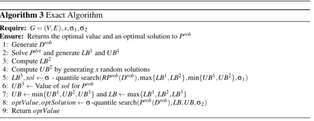
Our initial exact algorithm to solve Prob is presented in Algorithm 3. In a first step, all lower and upper bounds are computed and in a second step, a σ -quantile search is per-formed.
In the next section, we evaluate the computational efficiency of the proposed algorithm.
5.3 Experimental results
We implement the Exact Algorithm in Python 3.7 for two sets of instances: p-median in-stances from OR-Library and subgrids randomly generated.
We generate the distance matrices SP = (di j) and SPs= (ds
i j) for all scenario s ∈ V using networkx library 2.3. We execute our experiments on a server with 254Gb of RAM and 14
Algorithm 3 Exact Algorithm Require: G = (V, E), x, σ1, σ2
Ensure: Returns the optimal value and an optimal solution to Prob
1: Generate Drob
2: Solve Pdetand generate LB1and U B1 3: Compute LB2
4: Compute U B2by generating x random solutions
5: LB3, sol ← σ - quantile search(RProb(Drob), max{LB1, LB2}, min{UB1,U B2}, σ 1)
6: U B3← Value of sol for Prob
7: U B ← min{U B1,U B2,U B3} and LB ← max{LB1, LB2, LB3}
8: optValue, optSolution ← σ -quantile search(Prob(Drob), LB,U B, σ 2)
9: Return optValue
Intel Core (Haswell; no TSX) Processor at 2.3 Ghz. Mathematical programs are solved with CPLEX 12.9 (with MIPEmphasis option set to 0).
5.3.1 Experimental results on OR-Library Instances
The input data used for the computations are the 40 instances of the p-median problem from the OR-Library ([?]) which are used also for solving the p-center problem ([?,?]). n varies between 100 and 900 nodes and p varies between 5 and bn/3c. In the following we focus on the instances which could be solved within 5 hours.
Table 1 contains the value of the upper and lower bounds computed for the instances ordered by the number of their nodes and the value of p. We mark with an ∗ the values of the bounds that are equal to optimal value. It stands out that on all the instances con-sidered, LB3= U B3= v(Prob). The equality between U B3and LB3is not mandatory since only evacuation paths of a subset of nodes are considered in LB3. In fact, we record some instances in which LB3< v(Prob) (see in Figure 7) and, in these cases, the computation time is more important. The equality between LB3and U B3means that the evacuation distance of node s induces the radius of an optimal solution in scenario s. It may be due to the fact that OR-Library instances are considerably sparse.
Concerning lower bounds, LB2is also a tight lower bound very close and often equal to v(Prob), while LB1is the worst lower bound. Concerning upper bounds, U B1is globally better than U B2.
The Exact Algorithm computes all pairs of lower and upper bounds. In order to better understand the trade-off between bounds quality and computational time, we compare the processing time of three variants of the Exact Algorithm:
– EA1 is a version of the Exact Algorithm in which only LB1and U B1are computed, its processing time is TEA1. This variant is mainly based on the resolution of the determin-istic p-Center problem.
– EA2 is a version of the Exact Algorithm in which only LB2and U B2are computed, its processing time is TEA2. This variant is adapted from the Daskin’s algorithm for the RpCP.
– EA3 is a version of the Exact Algorithm in which only LB3and U B3are computed, its processing time is TEA3. This variant is a new one specific to RpCP and its evacuation strategy.
Instance n |E| p OPT LB1 UB1 LB2 UB2 LB3 UB3 pmed1 100 200 5 222 127 251 221 263 222* 222* pmed2 100 200 10 194 98 229 192 251 194* 194* pmed3 100 200 10 191 93 226 186 240 191* 191* pmed4 100 200 20 157 74 184 156 218 157* 157* pmed5 100 200 33 115 48 144 115* 180 115* 115* pmed6 200 800 5 180 84 208 180* 205 180* 180* pmed7 200 800 10 156 64 163 155 180 156* 156* pmed8 200 800 20 143 55 153 143* 188 143* 143* pmed9 200 800 40 124 37 136 124* 164 124* 124* pmed10 200 800 67 100 20 118 100* 136 100* 100* pmed11 300 1800 5 153 59 157 153* 169 153* 153* pmed12 300 1800 10 145 51 150 145* 171 145* 145* pmed13 300 1800 30 129 36 136 128 154 129* 129* pmed14 300 1800 60 116 26 125 115 145 116* 116* pmed15 300 1800 100 105 18 118 105* 133 105* 105* pmed16 400 3200 5 143 47 147 143* 153 143* 143* pmed17 400 3200 10 136 39 139 136* 150 136* 136* pmed18 400 3200 40 122 28 127 122* 144 122* 122* pmed19 400 3200 80 112 18 119 111 132 112* 112* pmed20 400 3200 133 103 13 113 103* 130 103* 103* pmed21 500 5000 5 137 40 139 137* 147 137* 137* pmed22 500 5000 10 133 38 137 133* 147 133* 133* pmed23 500 5000 50 118 22 122 118* 135 118* 118* pmed24 500 5000 100 110 15 115 110* 132 110* 110* pmed25 500 5000 167 103 11 113 103* 131 103* 103* pmed26 600 7200 5 134 38 137 134* 147 134* 134* pmed27 600 7200 10 128 32 132 128* 139 128* 128* pmed28 600 7200 60 114 18 118 114* 134 114* 114* pmed29 600 7200 120 108 13 113 108* 130 108* 108* pmed30 600 7200 200 103 9 109 103* 124 103* 103* pmed31 700 9800 5 128 30 136 124 135 128* 128* pmed32 700 9800 10 127 29 128 123 164 127* 127* pmed33 700 9800 70 113 15 119 110 126 113* 113* pmed34 700 9800 140 107 11 111 107* 125 107* 107* pmed35 800 12800 5 128 30 130 - 136 128* 128* pmed36 800 12800 10 125 27 127 - 134 125* 125* pmed37 800 12800 80 112 15 121 - 130 112* 112* pmed38 900 16200 5 127 29 129 - 138 127* 127* pmed39 900 16200 10 122 23 127 - 174 122* 122* pmed40 900 16200 90 111 13 113 - 123 111* 111*
Table 1: Optimal solution values and bound values for OR-Library instances
For pmed35 to pmed40, TEA1 and TEA2 exceed five hours: only EA3 can exactly solve all instances in less than 5 hours.
In Figure 6, we represent the processing times for instances from pmed1 to pmed34 for three different values of p: p = n/3 , p = n/10 and p = 10. For each p, three curves represent the processing times TEA1, TEA2 and TEA3, in function of n. We observe that our dedicated algorithm EA3 performs faster than EA1 and EA2. The reason is twofold: in EA1, the poor quality of the lower bound LB1(see Table 1) increases the number of iterations in step 8 of the Exact Algorithm. Conversely, in EA2 the quality of the lower bound LB2 highly decreases the number of iterations in step 8, however computing LB2 is very time consuming. More precisely, the generation of the input CPLEX instance for SCrob
p=n/3 p=n/10
p=10
Fig. 6: Processing time of each variant of the Exact Algorithm on some OR-Library instances
a large amount of time (at least 90% of the total computing time for generating LB2). On the other hand, LB3and U B3can be computed much faster while providing the best quality of bounds. Thus, EA3 is clearly the most efficient of the three algorithms.
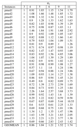
Once we have identified EA3 as the best of the three variants, we must verify whether improvements can be made by adjusting parameters σ1 and σ2. Given the quality of LB3, increasing σ2 to values greater than 3 is counterproductive: one iteration with σ -quantile search is enough to prove that the lower bound is an upper bound. In this case, increasing σ2 would only increase the size of the ILP model constructed in the step 8 of Exact Algorithm. However, we can potentially improve LB3processing time by using other values of σ1. Therefore, we compare the performance of algorithm EA3 on the 34 first instances from the OR-Library with different values of σ1 in a range of values between 3 and 11. For larger instances, computational times are not reported since they exceed 5 hours for some values of σ1. The results are given in Table 2, where, for each instance, the processing time of EA3 is standardised with respect to the processing time of EA3 for σ1= 3. Then we use the geometric mean to compare the average processing time for the different values of σ1. The experiment reveals that, with σ1= 4, EA3 is at least 14 percent faster than the other tested values for σ1.
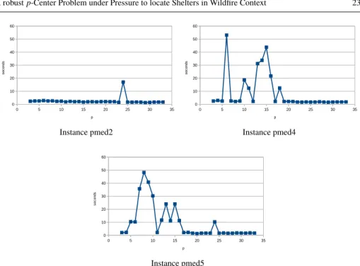
Then we perform a qualitative study to better understand the impact of p on the process-ing time. In Figure 7, the processprocess-ing time of EA3 is given for three instances with 100 nodes and 200 edges, named pmed1, pmed4 and pmed5. For each instance, the curve describes the evolution of TEA3 in function of p, with p ranging from 2 to 33. For pmed2, the processing
σ1 Instances 3 4 5 6 9 11 pmed1 1 0.91 1.03 1.15 1.54 1.79 pmed2 1 1.08 1.66 1.48 1.85 1.72 pmed3 1 0.98 1.32 1.34 1.18 1.94 pmed4 1 0.9 1.28 1.33 1.62 1.63 pmed5 1 0.82 1.03 0.98 1.39 1.29 pmed6 1 0.75 0.98 0.87 1.03 1.1 pmed7 1 1.46 1.84 1.91 1.68 2.92 pmed8 1 0.9 0.92 1.09 1.05 1.67 pmed9 1 0.82 0.88 1.12 1.66 1.41 pmed10 1 0.79 0.83 1.04 1.09 1.51 pmed11 1 0.81 0.9 0.89 1 1.26 pmed12 1 0.71 0.74 0.97 0.98 1.19 pmed13 1 0.82 1.47 1.47 0.93 1.69 pmed14 1 0.83 0.92 1.56 4.85 3.06 pmed15 1 1.04 1.07 1.39 1.29 1.89 pmed16 1 0.82 0.9 0.91 1.02 1.22 pmed17 1 0.91 0.98 0.99 1.08 1.27 pmed18 1 0.57 1.1 1.6 1.24 1.96 pmed19 1 0.67 0.94 0.88 1.24 3.86 pmed20 1 1.09 0.93 1.14 1.27 1.38 pmed21 1 0.86 0.9 0.94 1.45 1.24 pmed22 1 0.49 0.8 0.82 0.89 1.75 pmed23 1 0.72 1.39 2.73 2.59 1.69 pmed24 1 0.84 0.73 0.93 1.25 1.84 pmed25 1 2.26 1.64 2.57 3.68 3.73 pmed26 1 0.99 0.92 1.43 1.6 1.39 pmed27 1 0.29 1.22 0.82 0.59 0.58 pmed28 1 0.67 0.87 0.69 5.44 10.55 pmed29 1 0.6 0.53 0.61 2.25 1.33 pmed30 1 0.69 0.68 0.75 1.01 1.96 pmed31 1 1.34 1.2 1.35 1.47 1.96 pmed32 1 1.63 1.59 3.21 1.83 2.05 pmed33 1 1.33 2.21 1.23 3.77 1.38 pmed34 1 0.69 0.66 2.83 2.43 1.42 GEOMEAN 1 0.86 1.04 1.21 1.52 1.74
Table 2: Comparison of the standardized execution time of EA3 for different values of σ1
time is relatively stable for all values of p. On the contrary, the processing time to solve pmed4 and pmed5 is much more impacted by the variation of p. Precisely, processing times directly depend on the number of iterations to solve Probwith the σ -quantile search (step 8). When the number of iterations is equal to 1 (which corresponds to the case LB3= v(Prob)) the computation time is stable. But when LB3< v(Prob), the number of iterations increases (up to 5) and the computation time significantly increases.
These results underline that for a given size of instance, there is no obvious relationship between the value of p and the complexity of solving Prob.
Our experimental results allow to conclude that the original algorithm EA3 is the best one. In particular we are able to precisely tune the parameters defining Algorithm 4 called EA3*. The efficiency of EA3* comes from the quality of the lower bound obtained with a very efficient 4-quantile search algorithm. With such a bound, in most cases, only one iteration of the 3-quantile search is enough to determine an optimal solution of Probin step 5.
Instance pmed2 Instance pmed4
Instance pmed5
Fig. 7: Processing time of EA3 on three different instances for p ranging from 2 to 32 Algorithm 4 EA3*
Require: G = (V, E)
Ensure: Returns the optimal value and an optimal solution to Prob
1: Generate Drob= {Drob
1 , . . . , DrobTrob}
2: LB3, sol ← σ −quantile search(RProb(Drob), Drob 1 , DrobTrob, 4)
3: U B3← value of sol for Prob
4: optValue, optSolution ← σ −quantile search(Prob(Drob), LB3,U B3, 3)
5: Return optValue
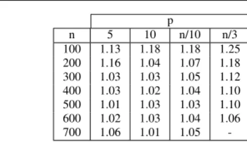
To measure the advantage of using RpCP over a classical deterministic p-Center prob-lem, we compare the value on the objective function of RpCP of an optimal solution of p-Center problem (referred to as deterministic solution) to the optimal solution value of RpCP. Let us recall that U B1exactly corresponds to the value, on RpCP, of a deterministic solution. Thus, we compute in Table 3 the ratio U B1/v(Prob) (none of the instances corre-spond to n=700 and p = n/3 in OR-Library). It appears that the gap can be quite significant, up to 25%. Consequently, the value of a deterministic solution can be far away from the optimal solution value of RpCP and better solutions can be found solving RpCP.
In the following, we report our experimental results on randomly generated subgrid instances.
5.3.2 Experimental results on random subgrid instances
As explained in Section 3.1, subgrids are relevant graphs for real case applications. Thus, we chose to test our algorithms on random subgrid instances. We generated a set of 18
sub-p n 5 10 n/10 n/3 100 1.13 1.18 1.18 1.25 200 1.16 1.04 1.07 1.18 300 1.03 1.03 1.05 1.12 400 1.03 1.02 1.04 1.10 500 1.01 1.03 1.03 1.10 600 1.02 1.03 1.04 1.06 700 1.06 1.01 1.05
-Table 3: Ratio between U B1and the optimal value of RpCP on OR-Library instances
grids along the following steps. From an original undirected unit grid of size (l × w), we generate three subgrids by randomly removing a node with probability 0.05, 0.1 and 0.2. For each subgrid, we remove isolated and leaf nodes being mandatory shelter locations. We apply this process to three grids of size 10 × 10, 20 × 10 and 20 × 20, into nine unit subgrids SG1, . . . , SG9. We then generate nine weighted subgrids wSG1, . . . , wSG9 by randomly as-signing length edge values, from 1 to 10, applied to the edges of SG1, . . . , SG9 respectively. The data set is available at [?].
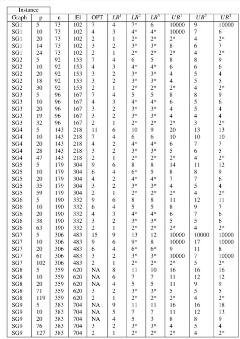
In the following, we present our synthetic analysis of the results. First, we solve Prob using Exact Algorithm with σ1= σ2= 3 and x = 10. Table 4 gives the values of the upper and lower bounds computed for the instances SG1, . . . , SG9 ordered by the number of their nodes and the value of p. Likewise, the values of the bounds that are equal to optimal values are marked with an ∗ . For bounds corresponding to non-feasible solutions for RpCP the value is 10000. In Table 4, NA denotes that the values cannot be computed within 5 hours. Please note that the best values achieved for the unsolved instances can be found in Table 10 in Appendix A.4. LB1is still the worst lower bound while LB2performs slightly better than LB3and both of them quite often reach optimal values. Concerning the upper bounds, we note that U B1and U B3are not so good as those of obtained for OR-Library instances.
Table 5 gives the value of the upper and lower bounds computed for the instances wSG1, . . . , wSG9 ordered by the number of their nodes and the value of p.
In the weighted case, LB2and LB3outperform LB1. Both lower bounds are not as good when the value of p is very low. U B3is the best upper bound sometimes reaching optimal value. In this case, the solution of RProbobtained with EA3 is also the optimal solution for Prob.
In Tables 8 and 9 in the Appendix A.4, we record the processing time of our algorithms on the unit subgrids and the weighted subgrids, for the fixed values of p (5,10 and 20), and relatives values of p (n/5 and n/3). For processing time exceeding 5 hours, we record NA. For each instance, the underlined value is the best. Overall, for both unit and weighted subgrids, EA3 is the most efficient algorithm.
In Tables 6 and 7, we record the ratio U B1/v(Prob) on the unit subgrids and the weighted subgrids. When the deterministic solution is not feasible, the corresponding ratio value is marked ∞. We observe that the gap, up to 167%, is larger than the one recorded for OR-Library instances. In Table 6, when p = n/3, the ratio U B1/v(Prob) equals 1 in all instances. In this case, we also have LB1= 1 which means that the optimal solution of the p-Center problem is a dominating set. We established the following result in [?]: if G is a planar triangle-free graph with no leaf nodes and C a dominating set, r(C) ≤ 2. Moreover, when
Instance
Graph p n |E| OPT LB1 LB2 LB3 U B1 U B2 U B3
SG1 5 73 102 7 4 7* 6 10000 9 10000 SG1 10 73 102 4 3 4* 4* 10000 7 6 SG1 20 73 102 2 1 2* 2* 2* 4 2* SG1 14 73 102 3 2 3* 3* 8 6 7 SG1 24 73 102 2 1 2* 2* 2* 4 2* SG2 5 92 153 7 4 6 5 8 8 9 SG2 10 92 153 4 3 4* 4* 6 6 6 SG2 20 92 153 3 2 3* 3* 4 5 4 SG2 18 92 153 3 2 3* 3* 4 5 5 SG2 30 92 153 2 1 2* 2* 2* 4 2* SG3 5 96 167 7 4 5 5 8 8 9 SG3 10 96 167 4 3 4* 4* 6 5 6 SG3 20 96 167 3 2 3* 3* 4 5 4 SG3 19 96 167 3 2 3* 3* 4 4 4 SG3 32 96 167 2 1 2* 2* 2* 3 2* SG4 5 143 218 11 6 10 9 20 13 13 SG4 10 143 218 7 4 6 6 10 10 10 SG4 20 143 218 4 2 4* 4* 6 7 7 SG4 28 143 218 3 2 3* 3* 5 6 5 SG4 47 143 218 2 1 2* 2* 2* 4 2* SG5 5 179 304 9 6 8 8 14 11 12 SG5 10 179 304 6 4 6* 5 8 8 9 SG5 20 179 304 4 2 4* 4* 7 7 6 SG5 35 179 304 3 2 3* 3* 4 5 4 SG5 59 179 304 2 1 2* 2* 2* 4 2* SG6 5 190 332 9 6 8 8 11 12 11 SG6 10 190 332 6 4 5 5 8 9 7 SG6 20 190 332 4 3 4* 4* 6 7 6 SG6 38 190 332 3 2 3* 3* 5 5 6 SG6 63 190 332 2 1 2* 2* 2* 4 2* SG7 5 306 483 15 9 13 12 10000 10000 10000 SG7 10 306 483 9 6 9* 8 10000 17 10000 SG7 20 306 483 6 4 6* 6* 9 11 8 SG7 61 306 483 3 2 3* 3* 10000 7 10000 SG7 102 306 483 2 1 2* 2* 2* 5 2* SG8 5 359 620 NA 8 11 10 16 16 16 SG8 10 359 620 NA 6 7 7 11 12 12 SG8 20 359 620 NA 4 5 5 11 9 9 SG8 71 359 620 3 2 3* 3* 5 5 5 SG8 119 359 620 2 1 2* 2* 2* 4 2* SG9 5 383 704 NA 9 11 11 16 16 18 SG9 10 383 704 NA 5 7 7 11 12 13 SG9 20 383 704 NA 4 5 3 8 8 9 SG9 76 383 704 3 2 3* 3* 4 5 4 SG9 127 383 704 2 1 2* 2* 2* 4 2*
Table 4: Optimal solution values and bound values for unit subgrids
p= n/3, there is no solution with radius equals to 1. So, the deterministic solution is an optimal solution for RpCP.
Instance
Graph p n |E| OPT LB1 LB2 LB3 U B1 U B2 U B3
wSG1 5 73 102 43 20 41 36 10000 50 10000 wSG1 10 73 102 25 12 24 23 29 39 26 wSG1 20 73 102 16 8 15 16* 19 30 16* wSG1 14 73 102 20 10 19 20* 29 31 22 wSG1 24 73 102 13 8 13* 13* 20 25 13* wSG2 5 92 153 29 17 29* 27 35 36 43 wSG2 10 92 153 20 11 20* 20* 25 27 26 wSG2 20 92 153 15 7 15* 15* 18 23 15* wSG2 18 92 153 16 7 16* 16* 19 23 19 wSG2 30 92 153 12 5 12* 12* 15 20 12* wSG3 5 96 167 27 14 26 25 35 35 39 wSG3 10 96 167 19 10 19* 19* 25 29 22 wSG3 20 96 167 15 7 15* 15* 20 20 15* wSG3 19 96 167 15 7 15* 15* 21 22 15* wSG3 32 96 167 11 5 11* 11* 15 19 11* wSG4 5 143 218 43 27 42 42 56 53 81 wSG4 10 143 218 31 16 30 29 39 41 41 wSG4 20 143 218 22 11 21 21 29 35 29 wSG4 28 143 218 17 8 17* 17* 25 29 25 wSG4 47 143 218 13 6 13* 13* 25 24 13* wSG5 5 179 304 39 25 38 37 51 48 45 wSG5 10 179 304 29 17 29* 28 33 39 33 wSG5 20 179 304 22 11 21 21 28 30 23 wSG5 35 179 304 17 8 17* 17* 24 27 29 wSG5 59 179 304 13 6 12 13* 24 24 13* wSG6 5 190 332 40 26 40* 39 48 55 45 wSG6 10 190 332 30 17 29 28 44 45 49 wSG6 20 190 332 21 11 21* 21* 33 37 40 wSG6 38 190 332 17 8 16 17* 21 27 17* wSG6 63 190 332 13 6 13* 13* 19 22 13* wSG7 5 306 483 67 38 65 59 10000 10000 10000 wSG7 10 306 483 44 26 44* 43 10000 88 10000 wSG7 20 306 483 32 17 32* 31 10000 62 10000 wSG7 61 306 483 17 8 17* 17* 10000 35 10000 wSG7 102 306 483 13 6 13* 13* 10000 30 10000 wSG8 5 359 620 53 34 47 44 69 70 71 wSG8 10 359 620 38 23 35 35 51 53 52 wSG8 20 359 620 28 16 27 27 35 40 32 wSG8 71 359 620 17 8 17* 17* 22 29 19 wSG8 119 359 620 13 6 13* 13* 17 24 13* wSG9 5 383 704 58 34 47 46 79 68 81 wSG9 10 383 704 38 23 36 36 51 51 59 wSG9 20 383 704 28 17 27 27 39 44 35 wSG9 76 383 704 17 8 16 17* 22 29 19 wSG9 127 383 704 13 6 13* 13* 17 24 13*
Table 5: Optimal solution values and bound values for weighted subgrids
6 Conclusion
We introduce a new version of the p-Center problem motivated by the context of evacuation in case of wildfires. We call it the Robust p-Center problem under Pressure and emphasize its differences with the existing models in the literature. We study the complexity of this problem: we show that RpCP is NP-hard in all hereditary classes of graphs where the