A new class of problems in the calculus of variations
Ivar Ekeland
1∗,
Yiming Long
2†,
Qinglong Zhou
2‡ 1CEREMADE and Institut de Finance
Universit´
e de Paris-IX, Dauphine, Paris, France
2
Chern Institute of Mathematics and LPMC
Nankai University, Tianjin 300071, China
June 19, 2013
Dedicated to Professor Alain Chenciner on his 70th birthday
1
Introduction
In economic theory, and in optimal control, it has been customary to discount future gains at a constant rate δ > 0. If an individual with utility function u (c) has the choice between several streams of consumption c (t), 0 ≤ t, he or she will choose the one which maximises the present value, given by:
∫ ∞ 0
u (c (t)) e−δtdt (1)
That future gains should be discounted is well grounded in fact. On the one hand, humans prefer to enjoy goods sooner than later (and to suffer bads later than sooner), as every child-rearing parent knows. On the other hand, it is also a reflection of our own mortality: 10 years from now, I may simply no longer be around to enjoy whatever I have been promised. These are two good reasons why people are willing to pay a little bit extra to hasten the delivery date, or will require compensation for postponement, which is the essence of discounting.
On the other hand, there is no reason why the discount rate should be constant, i.e. why the discount factor should be an exponential e−δt. The practice probably arises from the compound
interest formula limε→0(1 − εδ)t/ε = e−δt, when a constant interest rate δ is assumed, but even in
finance, interest rates vary with the horizon: long-term rates can be widely different from short-term ones. As for economics, there is by now a huge amount of evidence that individuals use higher discount rates for the near future than for the long-term (see [18] for a review up to 2002). There
∗E-mail: [email protected]
†Partially supported by NNSF, MCME, RFDP, LPMC of MOE of China, and Nankai University. E-mail:
‡Partially supported by the Chern Institute of Mathematics, Nankai University, CEREMADE of Universit´e Paris
is also an aggregation problem: in a society where individuals use constant (but different) discount rates, the collective discount rate may be non-constant (see [14]). So the present value formula (1) should be replaced by the more general one:
∫ ∞ 0
u (c (t)) h (t) dt (2)
where h is a decreasing function, with h (0) = 1.
But then a new problem arises, which is now well recognized in economic theory, but to our knowledge has not yet received the attention it deserves in control theory. It is the problem of time-inconsistency, which runs as follows. Suppose the decision-maker has the choice between two streams of consumption c1(t) and c2(t), starting at time T > 0. At time t = 0, he or she finds c1(t)
yields the highest present value: ∫ ∞ T u (c1(t)) h (t) dt > ∫ ∞ T u (c2(t)) h (t) dt. (3)
He or she then chooses c1(t). When time T is reached, the present values are now:
∫ ∞ T u (c1(t)) h (t − T ) dt and ∫ ∞ T u (c2(t)) h (t − T ) dt (4)
If h (t) = e−δt, then the ordering found at time t = 0 will persist at time t = T . Indeed:
∫ ∞ T u (c (t)) e−δ(t−T )dt = eδT∫ ∞ T u (c (t)) e−δtdt
so that the two terms in (4) are proportional to the two terms in (3). However, this is a peculiarity of the exponential function, and it is not to be expected with more general discount rates. The decision-maker then faces a basic rationality problem: what should he or she do ? To be more specific, assume the state k (t) is related to the control c (t) by the dynamics:
dk
dt = f (k) − c (t) , k (0) = k0 (5)
c (t) ≥ 0, k (t) ≥ 0 (6)
and the decision-maker is interested in maximising (2). How should he or she behave ?
In the exponential case, when h (t) = e−δt, the answer is to pick the optimal solution: if it is
optimal at time t = 0, it will still be optimal at all times T > 0 (this, by the way, is the content of the dynamic programming principle). But in the non-exponential case, the notion of optimality changes with time: each observer, from time t = 0 on, has his or her own optimal solution. No one agrees on what the optimal solution is, so optimality no longer provides an answer to the decision-making process, and one must look for other concepts to describe rational behaviour.
A clear requirement for rationality is that any strategy put forward be implementable. Suppose a Markov strategy c = σ (k) is put forward at time t = 0. If it is to be followed at all later times t > 0, then it must be the case that the decision-maker at that time finds no incentive to deviate. More precisely, if he/she assumes that at all later times the strategy (closed-loop feedback) c = σ (k) will be applied, then he/she should find it in his/her interest to apply σ as well. In other words, σ
should be a subgame-perfect Nash equilibrium of the leader-follower game played by the successive decision-makers. This idea has been introduced by Phelps ([29], [30]) in models with discrete time (see [24] and [27] for further developments), and adapted by Karp ([22], [23]), and by Ekeland and Lazrak ([12], [13], [14], [16]) to the case of continuous time.
In this paper, we will follow the approach by Ekeland and Lazrak. It consists of introduc-ing a value function V (k), which is very similar to the value function in optimal control, and of showing that it satisfies a functional-differential equation which is reminescent of the Hamilton-Jacobi-Bellman (HJB) of optimal control. Conversely, any solution of that equation with suitable boundary conditions will give us an equilibrium strategy.
In the work by Ekeland and Lazrak, this approach was applied to (2), with h (t) = α exp (−r1t) +
(1 − α) exp (−r2t), and it was showed that the corresponding problem had a continuum of
equilib-rium strategies. In the present paper, in view of applications to economics, and of the mathematical interest, we aim to extend the analysis to the more general case:
(1 − α) ∫ ∞ 0 e−r1t u (c (t) , k (t)) dt + α ∫ ∞ 0 e−r2t U (c (t) , k (t)) dt (7)
As a by-product of our analysis, we will treat the problem: (1 − α) δ
∫ ∞ 0
e−δtu (c (t) , k (t)) dt + α lim
t→∞U (k (t) , c (t)) (8)
which was introduced by Chichilnisky (see [10], [11]) to model sustainable development. Note that, if u (c, k) ≥ 0 and:
sup {U (c, k) | c > 0, k > 0, c = f (k)} = ∞
then maximising (8) under the dynamics (5), (6) leads to the value +∞, so that optimisation is clearly not an answer to the problem. Instead, we find equilibrium strategies. To our knowledge, this is an entirely new result. We show that there is a continuum of such strategies. More precisely, there is a continuum of points k∞ which can be realized as the long-term level of capital by an
equilibrium strategy. This support, however, is one-sided, that is, k∞ can be reached only from the
initial level of capitals k0 lying on its left (or from its right). To our knowledge, this is the first time
such strategies have been identified.
The structure of the paper is as follows. In the next section, we consider the problem of max-imising
∫ ∞ 0
e−δtu (c (t) , k (t)) dt (9)
under the dynamics (5), (6), and we show that it has a solution. On the way, we introduce the corresponding HJB equation, and we show that it has a C2 solution. Next, we define equilibrium
strategies. With each such strategy we associate a value function V (k), and we show that it satisfies an integro-differential equation which generalizes the HJB equation, and we prove a verification theorem: any solution of this equation with suitable boundary conditions gives an equilibrium strategy. We show that the trajectories satisfy an integro-differential equation which generalizes the classical Euler-Lagrange equations, and we connect the Ekeland-Lazrak approach with the Karp approach.
In section 4, we apply the theory to problem (7), and show that it has a continuum of equilibrium strategies, thereby extending the results of [14]. It should be noted that the equations for V (k) are
given in implicit form, that is, they cannot be solved with respect to V′
(k), so that finding a C2
solution requires special techniques (first a blow-up, and then the central manifold theorem). We then consider the criterion:
(1 − α) δ ∫ ∞ 0 e−δtu (c (t) , k (t)) dt + αr∫ ∞ 0 e−rtU (c (t) , k (t)) dt (10)
which belongs to the class (7) and we let r → 0. In the limit, we get equilibrium strategies for the Chichilnisky problem (8), which we describe explicitly.
2
The Ramsey problem
This is the classical model for economic growth, originating with the seminal paper of Ramsey [31] in 1928, and developed by Cass [9], Koopmans [25] and many others (see [5] for a modern exposition). We are given a point k0> 0 and a concave continuous function f on [0, ∞), which is C∞on ]0, ∞[
and satisfies the Inada conditions: lim x→0f ′ (x) = +∞, lim x→∞f ′ (x) ≤ 0. (11)
Definition 1 A capital-consumption path (c (t) , k (t)) , t ≥ 0, is admissible if:
k (t) > 0 and c (t) > 0 for all t, (12)
dk
dt = f (k) − c, k (0) = k0, (13)
The set of all admissible paths starting from k0 (i.e, such that k (0) = k0) will be denoted by
A (k0).
We are given a number δ > 0 and another concave, increasing function u on ]0, ∞), which is C∞
on the interior, with u′′
(c) > 0 everywhere. We introduce the following criterion on A (k0):
I (c, k) = ∫ ∞
0
u(c(t), k(t))e−δtdt, (14)
and we consider the optimization problem:
sup {I (c, k) | (c, k) ∈ A (k0)} . (15)
The Euler-Lagrange equation is given by: u′′ 11 dc dt = (δ − f ′ (k)) u′ 1− u ′ 2− (f (k) − c) u ′′ 12. (16)
Equation (16), together with equation (13), constitute a system of two first-order ODEs for the unknown functions (c (t) , k (t)). In the particular case when u = u (c) does not depend on k, the last equation simplifies to:
u′′ 11 dc dt = (δ − f ′ (k)) u′ 1
and the (16), (13) gives rise to a well-known phase diagram, with a hyperbolic stationary point (c∞, k∞) characterized by f
′
problem in that case then is the solution of (16), (13) which converges to (c∞, k∞) (see [5] for
instance).
In the general case where u (c, k) depends on k, the situation is not as simple, and to our knowledge has not been investigated. Stationary points (c∞, k∞) of the dynamics (if any) are given
by: c∞− f (k∞) = 0 (17) (δ − f′ (k∞)) u ′ 1(f (k∞) , k∞) − u ′ 2(f (k∞) , k∞) = 0. (18)
To prove the existence of an optimal strategy, we do not use the Euler equation. We use the Hamilton-Jacobi-Bellman (HJB) equation instead. Introduce the optimal value as a function of the initial point:
V (k0) := sup {I (c, k) | (c, k) ∈ A (k0)}
If there is an optimal solution (c (t) , k (t)), and it converges to (c∞, k∞) when t → ∞, then,
substituting in (14), we must have: V (k∞) = ∫ ∞ 0 e−δtu (c ∞, k∞) dt = 1 δu (c∞, k∞) = 1 δu (f (k∞) , k∞) (19) Theorem 2 If V (k) is C1, it satisfies the HJB equation, namely:
δV (k) = max
c {u(c, k) + (f (k) − c)V ′
(k)}. (20)
Conversely, suppose the HJB equation has a C2 solution satisfying (19) for some (c
∞, k∞), and
define a strategy c = σ (k) by:
u′
1(σ (k) , k) = V ′
(k) (21)
Suppose moreover that the solution of: dk
dt = f (k) − σ (k) , k (0) = k0, (22)
converges to k∞for all initial points k0. Then σ (k) is an optimal solution of the generalized Ramsey
problem (15)
This is the so-called verification theorem, which is classical (see [4]). We need V to be C2, so
that σ is defined. Since u′′
1 > 0, we can use the implicit function theorem on equation (21) to define
σ. If V is C2, then σ is C1, and the initial-value problem (22) has a unique solution. Note also that
everything is local: the functions V and σ are defined in some neighbourhood of k∞ only, and the
initial value k0 is assumed to belong to that neighbourhood of k∞.
So, to prove the (local) existence of an optimal strategy σ (k), we have to prove that the HJB equation has a C2 solution V with V (k
∞) = δ
−1u (f (k
∞) , k∞), and that the corresponding path
k (t) converges to k∞. Then the right-hand side of (22) converges to 0, so that c (t) = σ (k (t))
Theorem 3 Suppose there is some k∞> 0 satisfying (18) and: u′ 1f ′′ + u′′ 22+ f ′ ( u′′ 12− u′ 2 u′ 1 u′′ 11 ) −u ′ 2 u′ 1 u′′ 12< 0 (23)
(all values to be taken at k∞ and c∞ = f (k∞)). Then there is an optimal strategy c = σ (k)
converging to k∞
If u = u (c) does not depend on k, then u′
2 = 0. Equation (18) becomes f ′
(k∞) = δ,
which defines k∞ uniquely because of the Inada conditions (11) on f , and condition (23) becomes
u′ 1(c∞) f
′′
(k∞) < 0, which is satisfied automatically. So there is an optimal strategy in that case,
and one can even show that it is globally defined. For u depending on k, however, the situation is different.
Proof. We follow the method of [15]. By the inverse function theorem, the equation u′
1(c, k)) = p
defines c as a C1 function of p and k:
c = φ(p, k), u′
1(φ(p, k), k)) = p (24)
We rewrite (20) as a Pfaff system:
dV = pdk, (25)
p(f (k) − φ(p, k)) + u(φ(p, k), k) = δV, (26)
and we seek a C2solution V satisfying:
V (k∞) =
1
δu(f (k∞), k∞). (27)
Differentiating (26) leads to:
δdV = (f (k) − φ(p, k))dp + pf′
(k)dk + u′
2(φ(p, k), k)dk (28)
Plugging (28) into (25), we get:
(f (k) − φ(p, k))dp = (δp − pf′
(k) − u′
2(φ(p, k), k))dk. (29)
Introducing an auxiliary variable t, we rewrite this as a system of two ODES for two functions p (t) and k (t): dk dt = f (k) − φ(p, k) dp dt = δp − pf ′ (k) − u′ 2(φ(p, k), k) (30) with the initial condition
(k(0), p(0)) = (k∞, p∞) By (24), we must have p∞= u ′ 1(φ(p∞, k∞), k∞) = u ′ 1(c∞, k∞) = u ′ 1(f (k∞) , k∞)
Differentiating (24) with respect to p and k respectively, we derive the formulas: φ′ 1(p∞, k∞) = 1 u′′ 11(φ(p∞, k∞), k∞) = 1 u′′ 11(f (k∞), k∞) , (31) φ′ 2(p∞, k∞) = − u′′ 11(φ(p∞, k∞), k∞) u′′ 11(φ(p∞, k∞), k∞) = −u ′′ 12(f (k∞), k∞) u′′ 11(f (k∞), k∞) , (32)
We can now linearizd (30) at the point (p∞, k∞). We get:
d dt ( k − k∞ p − p∞ ) = A∞ ( k − k∞ p − p∞ ) . where the constant matrix A∞ is given by:
A∞:= f′ +u ′′ 12 u′′ 11, − 1 u′′ 11 −u′ 1f ′′ − u′′ 22+ (u′′ 12) 2 u′′ 11 , δ − f ′ −u ′′ 12 u′′ 11 .
and all the values are to be taken at (k∞, p∞). The characteristic polynomial is:
λ2− δλ − [u ′ 1∞f ′′ ∞+ u ′′ 22∞ u′′ 11∞ + f′ ∞( u′′ 12∞ u′′ 11∞ −u ′ 2∞ u′ 1∞ ) −u ′ 2∞ u′ 1∞ u′′ 12∞ u′′ 11∞ ] = 0 where we used f′ ∞+ u′ 2∞ u′
1∞ = δ by (17). Because of assumption (23), it has two real roots with
different signs, λ+> 0 and λ−< 0. Thus (k∞, p∞) is a hyperbolic fixed point of (30), with a stable
C∞
-manifold S which corresponds to λ−and an unstable C ∞
-manifold U which corresponds to λ+.
Choose a smooth parametrization (ks(x), ps(x)) for the curve S. The tangent at the fixed point is:
dps dks (k∞) = u ′′ 11(f ′ ∞− λ−) + u ′′ 12
and plugging k = ks(x), p = ps(x) into equation (26), we get
Vs=ps(x)(f (ks(x)) − φ(ps(x), ks(x))) + u(φ(ps(x), ks(x)), ks(x))
δ .
Moreover, differentiating (26), and using (23) again, we find: dVs
dks
(k∞) = u ′
1(f (k∞), k∞) > 0,
It follows that the curve in parametric form x → (k (x) , V (x)) is in fact the graph of a function V (k) which solves HJB and satisfies (27). By (25), we have
d2V s dks2 (k∞) = dps dks (k∞) = u ′′ 11∞(f ′ ∞− λ−) + u ′′ 12∞. (33)
It remains to show that the strategy σ defined by u′ 1(σ (k) , k) = V ′ (k) converges to (f (k∞) , k∞). We rewrite σ as: σ(k) = φ(V′ (k), k). Linearizing the equation
dk dt = f (k) − c = f (k) − φ(V ′ (k), k) gives d(k − k∞) dt = λ−(k − k∞) and this concludes the proof.
Let us show how to deduce the Euler equation (16) from the HJB equation (20) and the optimal strategy (21). Setting c (t) := σ (k (t)), differentiating (20) with respect to k, and applying the envelope theorem, we get:
δV′ (k) = u′ 2(c, k) + f ′ (k) V′ (k) + (f (k) − c) V′′ (k) , and hence, noting that dk
dt = f (k) − c (t) : (δ − f′ (k)) V′ (k) − u′ 2(c, k) = (f (k) − c) d dkV ′ (k) = d dtV ′ (k) . Replacing V′ (k) by u′ 1(σ (k) , k) = u ′ 1(c, k), we get: (δ − f′ (k)) u′ 1(c, k) − u ′ 2(c, k) = d dtu ′ 1(c, k),
which is precisely the Euler equation.
3
Time-inconsistency.
3.1
Equilibrium strategies
We consider the intertemporal decision problem (as it seen at time t = 0) J (c, k) =
∫ ∞ 0
[h (t) u (c (t) , k (t)) + H (t) U (c (t) , k (t))] dt (34) under the dynamics described by (5) and (6). Here h and H are discount factors, i.e. C∞
non-increasing functions on [0, ∞), such that h (0) = H (0) = 1 and h (∞) = H (∞) = 0, while u and U are utility functions. They are assumed to be C∞
on ]0, ∞)2, with u′′
< 0 and U′′
< 0 everywhere. We shall also assume that they decay exponentially, so that there is some ρ > 0 and some T > 0 such that h (t) < e−ρtand H (t) < e−ρtfor t ≥ T .
Because of time-inconsistency, the decision problem can no longer be seen as an optimization problem. There is no way for the decision-maker at time 0 to achieve what is, from her point of view, the first-best solution of the problem, and she must turn to a second-best policy: the best she
can do is to guess what her successor are planning to do, and then to plan her own consumption c(0) accordingly. In other word, we will be looking for a subgame-perfect equilibrium of the leader-follower game played by successive generations.
The equilibrium policy was described in [14] for the case when the criterion (34) did not include the second term, and u did not depend on k. We will extend this analysis to the present situation, and then compare it with the approach in [22].
Definition 4 A Markov strategy c = σ (k) is convergent if there is a point k∞ and a neighbourhood
N of k∞such that, for every k0∈ N the solution k(t) of (22) converges to k∞(and so c (t) = σ (k (t))
converges to c∞= f (k∞)). If this is the case, we shall say that (c∞, k∞) is supported by σ.
Let us suppose that a convergent Markov strategy σ has been announced and is the public knowledge σ. The decision-maker at T has capital stock kT. If all future decision-maker apply the
strategy σ, the resulting future capital stock flow k(t) obeys: dk
dt = f (k) − σ (k) , k (T ) = kT, T ≤ t (35)
Since every decision-maker faces the same problem (with different stock levels) it is enough to take T = 0. Suppose the decision-maker at time 0 holds power for 0 ≤ t < ε, and expects all later decision-makers to apply the strategy σ. He or she then explores whether it is in his or her interest to apply the strategy σ, that is, to play c0= σ (k0) for 0 ≤ t < ε. If he or she applies the constant
control c for 0 ≤ t ≤ ε.
Suppose the constant control c is use on 0 ≤ t ≤ ε. The immediate utility flow during [0, ε] is [u(c, k0) + U (c, k0)]ε + o(ε) where o(ε) is a higher order term of ε. At time ε, the resulting capital
will be k0+ (f (k0) − c)ε + o(ε). From then on, the strategy σ will be applied, which results in a
capital stock kc satisfying (we omit higher-order terms):
dkc
dt = f (kc) − σ (kc) , kc(ε) = k0+ (f (k0) − c)ε, t ≥ ε (36) The capital stock kc can be written as
kc(t) = k0(t) + k1(t)ε, (37)
where k0(t) is the unperturbed solution, and k1(t) is given by the linearized equation:
dk0 dt = f (k0) − σ (k0) , k0(0) = k0 (38) dk1 dt = (f ′ (k0) − σ′(k0)) k1, k1(0) = σ (k0) − c (39)
Evaluating the integral (34) we get: J (ε) = u(c, k0)ε +∫ ∞ ε h(s)u(σ(k0(t) + εk1(t)), k0(t) + εk1(t))dt +U (c, k0)ε +∫ ∞ ε H(s)U (σ(k0(t) + εk1(t)), k0(t) + εk1(t))dt
Letting ε → 0, so that commitment span of the decision-maker vanishes, we get: lim
ε→0
1
where P (k0, σ, c) = u(c, k0) − u(σ(k0), k0) + (U (c, k0) − U (σ(k0), k0)) + ∫ ∞ 0 h(t)u′ 1(σ(k0(t)), k0(t))σ′(k0(t))k1(t)dt + ∫ ∞ 0 h(t)u′ 2(σ(k0(t)), k0(t))k1(t)dt + ∫ ∞ 0 H(t)U′ 1(σ(k0(t)), k0(t))σ′(k0(t))k1(t)dt + ∫ ∞ 0 H(t)U′ 2(σ(k0(t)), k0(t))k1(t)dt,
Definition 5 A convergent Markov strategy σ is an equilibrium if we have: max
c P (k, σ, c) = P (k, σ, σ (k)), ∀k.
3.2
The HJB approach
We now characterizes the equilibrium strategy. We write kc(t) = K(t; k0, σ) where K is the flow
associated with the differential equation (38). We also define a function φ by: u′ 1(φ(x, k), k) + U ′ 1(φ(x, k), k) = x, φ(u′ 1(c, k) + U ′ 1(c, k), k) = c Since u′′ 1and U ′′
1 are both negative, the function φ is well-defined by the implicit function theorem.
Theorem 6 Let σ be an equilibrium strategy. The function: V (k0) = ∫ ∞ 0 h(t)u(σ(K(t; k0, σ)), K(t; k0, σ))dt + ∫ ∞ 0 H(t)U (σ(K(t; k0, σ)), K(t; k0, σ))dt (40)
satisfies the integral equation: V (k0) =∫ ∞ 0 h(t)u(φ ◦ V ′ (K(t; k0, φ ◦ V′)), K(t; k0, φ ◦ V′))dt +∫∞ 0 H(t)U (φ ◦ V ′ (K(t; k0, φ ◦ V′)), K(t; k0, φ ◦ V′))dt (IE)
and the instantaneous optimality condition u′
1(σ(k0), k0) + U1′(σ(k0), k0) = V′(k0), σ(k0) = φ(V′(k0), k0), (41)
Conversely, suppose a function V is twice continuously differentiable, satisfies (IE), and the strategy σ(k0) := φ(V′(k0), k0) is convergent. Then σ is an equilibrium strategy.
For the sake of convenience, we have shortened σ(k0) := φ(V′(k0), k0) to σ = φ ◦ V′.
Proof. Since the system is autonomous, we have:
K(s; K(t; k0, σ), σ) = K(s + t; k0, σ). (42)
Next, denote the fundamental solution of the linearized equation of (35) at k0 by R(k0; t) so
that: k1(t) = R(k0; t)(σ(k0) − c) dR dt = (f ′ (K(t; k0, σ)) − σ′(K(t; k0, σ)))R(t), R(k0; 0) = I,
R and K are related by: ∂K(t; k0, σ) ∂k0 = R(k0; t), (43) ∂K(t; k0, σ) ∂t = f (K(t; k0, σ)) − σ(K(t; k0, σ)). (44)
Let us now turn to the first part of the theorem. Differentiating (40)with respect to k0:
V′ (k0) = ∫ ∞ 0 h(t)u′ 1(σ(K(t; k0, σ)), K(t; k0, σ))σ ′ (K(t; k0, σ))R(k0; t)dt + ∫ ∞ 0 h(t)u′ 2(σ(K(t; k0, σ)), K(t; k0, σ))R(k0; t)dt + ∫ ∞ 0 H(t)U′ 1(σ(K(t; k0, σ)), K(t; k0, σ))σ′(K(t; k0, σ))R(k0; t)dt + ∫ ∞ 0 H(t)U′ 2(σ(K(t; k0, σ)), K(t; k0, σ))R(k0; t)dt. (45)
Substituting k0(t) = K(t; k0, σ) and k1(t) in the definition of P , we get:
P (k0, σ, c) = [u(c, k0) + U (c, k0)] − [u(σ(k0), k0) + U (σ(k0), k0)] + ∫ ∞ 0 h(t)u′ 1(σ(K(t; k0, σ)), K(t; k0, σ))σ′(K(t; k0, σ))R(k0; t)(σ(k0) − c)dt + ∫ ∞ 0 h(t)u′ 2(σ(K(t; k0, σ)), K(t; k0, σ))R(k0; t)(σ(k0) − c)dt + ∫ ∞ 0 H(t)U′ 1(σ(K(t; k0, σ)), K(t; k0, σ))σ ′ (K(t; k0, σ))R(k0; t)(σ(k0) − c)dt + ∫ ∞ 0 H(t)U′ 2(σ(K(t; k0, σ)), K(t; k0, σ))R(k0; t)(σ(k0) − c)dt.
Since u and U are strictly concave and differentiable with respect to c, the necessary and sufficient condition to maximize P (k0, σ, c) with respect to c is that the derivative vanishes at c = σ(k0), that
is: u′ 1(σ(k0), k0) + U1′(σ(k0), k0) = ∫ ∞ 0 h(t)u′ 1(σ(K(t; k0, σ)), K(t; k0, σ))σ′(K(t; k0, σ))R(k0; t)dt + ∫ ∞ 0 h(t)u′ 2(σ(K(t; k0, σ)), K(t; k0, σ))R(k0; t)dt + ∫ ∞ 0 H(t)U′ 1(σ(K(t; k0, σ)), K(t; k0, σ))σ ′ (K(t; k0, σ))R(k0; t)dt + ∫ ∞ 0 H(t)U′ 2(σ(K(t; k0, σ)), K(t; k0, σ))R(k0; t)dt,
The right-hand side is precisely V′
(k0), as we wanted. Therefore, the equilibrium strategy satisfies
u′ 1(σ(k0), k0) + U ′ 1(σ(k0), k0) = V ′ (k0)
and we have σ(k0) = φ(V′(k0), k0). Substituting back into equation (40), we get the functional
equation (IE). This prove the first part of the theorem (necessity). We refer to [14] for the second part (sufficiency).
The following theorem gives an alternative characterization, the differential equation, which resembles the usual HJB equation from the calculus of variation.
Theorem 7 Let V be a C2 function such that the strategy σ = φ ◦ V′
converges to ¯k. Then V satisfies the integral equation (IE) if and only if it satisfies the following integro-differential equation
u(φ ◦ V′ (k0), k0) + U (φ ◦ V′(k0), k0) + V′(k0)(f (k0) − φ(V′(k0), k0)) = −∫∞ 0 h ′ (t)u(φ ◦ V′ (K(t; k0, φ ◦ V′)), K(t; k0, φ ◦ V′))dt −∫∞ 0 H ′ (t)U (φ ◦ V′ (K(t; k0, φ ◦ V′)), K(t; k0, φ ◦ V′))dt (DE) together with the boundary condition
V (¯k) = u(f (¯k), ¯k) ∫ ∞ 0 h(t)dt + U (f (¯k), ¯k) ∫ ∞ 0 H(t)dt. (BC)
Proof. Introduce the function ϕ defined by ϕ(k0) = V (k0) − ∫ ∞ 0 h(t)u(σ(K(t; k0, σ)), K(t; k0, σ))dt − ∫ ∞ 0 H(t)U (σ(K(t; k0, σ)), K(t; k0, σ))dt,
where σ(k0) = φ(V′(k0), k0). Consider the value ψ(t, k0) of ϕ along the trajectory t → K(t; k0, σ)
originating from k0 at time 0, that is
ψ(t, k0) = ϕ(K(t; k0, σ)) = V (K(t; k0, σ)) − ∫ ∞ t h(s − t)u(σ(K(σ; s, k0)), K(σ; s, k0))ds − ∫ ∞ t H(s − t)U (σ(K(σ; s, k0)), K(σ; s, k0))ds,
Then the derivative of ψ with respect to t is given by: ∂ψ(t, k0) ∂t =V ′ (Kt)[f (Kt) − φ ◦ V ′ (Kt)] + u(φ ◦ V ′ (Kt), Kt) + U (φ ◦ V ′ (Kt), Kt) + ∫ ∞ 0 h′ (s)u(φ ◦ V′ (K(s; Kt, φ ◦ V′)), K(s; Kt, φ ◦ V′))ds + ∫ ∞ 0 H′ (s)U (φ ◦ V′ (K(s; Kt, φ ◦ V′)), K(s; Kt, φ ◦ V′))ds,
where we have denoted K(t; k0, φ ◦ V′) by Ktfor convenience. If (DE) holds, then the right hand side
is identically zero along the trajectory, so that ψ(t, k0) does not depend on t, thus ψ(s, k0) = ψ(t, k0)
for all s, t ≥ 0. Letting t → ∞ in the definition of ψ, we get ψ(s, k0) = lim t→∞ψ(t, k0) = V (¯k) − ∫ ∞ 0 h(s)u(σ(¯k), ¯k)ds − ∫ ∞ 0 H(s)U (σ(¯k), ¯k)ds, (46) and hence, if (BC) holds, then ψ = ϕ ≡ 0 and so equation (IE) holds. Conversely, if V (k) satisfies equation (IE), then the same lines of reasoning shows that equation (DE) and the boundary condition (BC) are satisfied.
3.3
The Euler equations
To obtain the Euler-Lagrange-like equation, we differentiate the both side of (DE) with respect to k0. We get: − ∫ ∞ 0 h′ (t)u′ 1(σ(K(t; k0, σ)), K(t; k0, σ))σ ′ (K(t; k0, σ)) ∂K(t; k0, σ) ∂k0 dt − ∫ ∞ 0 h′ (t)u′ 2(σ(K(t; k0, σ)), K(t; k0, σ)) ∂K(t; k0, σ) ∂k0 dt − ∫ ∞ 0 H′ (t)U′ 1(σ(K(t; k0, σ)), K(t; k0, σ))σ ′ (K(t; k0, σ)) ∂K(t; k0, σ) ∂k0 dt − ∫ ∞ 0 H′ (t)U′ 2(σ(K(t; k0, σ)), K(t; k0, σ))∂K(t; k0, σ) ∂k0 dt = [u′ 1(σ(k0), k0) + U ′ 1(σ(k0), k0)]σ ′ (k0) + u ′ 2(σ(k0), k0) + U ′ 2(σ(k0), k0) + V′ (k0)f′(k0) − V′(k0)σ′(k0) + V′′(k0)(f (k0) − σ(k0)).
Plugging k0= k(t), σ(k(t)) = c(t) and using (41) to cancel the first and the fifth terms, together
with (13) and (43), we have − ∫ ∞ 0 h′ (s)u′ 1(σ(K(s; k(t), σ)), K(s; k(t), σ))σ ′ (K(s; k(t), σ))R(k (t) , s)ds − ∫ ∞ 0 h′ (s)u′ 2(σ(K(s; k(t), σ)), K(s; k(t), σ))R(k (t) , s)ds − ∫ ∞ 0 H′ (s)U′ 1(σ(K(s; k(t), σ)), K(s; k(t), σ))σ ′ (K(s; k(t), σ))R(k (t) , s)ds − ∫ ∞ 0 H′ (s)U′ 2(σ(K(s; k(t), σ)), K(s; k(t), σ))R(k (t) , s)ds = u′ 2(c(t), k(t)) + U ′ 2(c(t), k(t)) + V ′ (k(t))f′ (k(t)) + V′′ (k(t))(f (k(t)) − c(t)) = u′ 2(c(t), k(t)) + U ′ 2(c(t), k(t)) + [u ′ 1(c(t), k(t)) + U ′ 1(c(t), k(t))]f ′ (k(t)) + d dt[u ′ 1(c(t), k(t)) + U ′ 1(c(t), k(t))],
where to get the last two terms in the right hand side, we have used (41) again. We have K(s; k(t), σ) = k(s + t), and R(k (t) ; s) = R(k0; s + t) σ′ (k (t)) = 1 f (k(t)) − c(t) dc dt (47) R(k0; s + t) = exp(f ′ (k (t)) − 1 f (k(t)) − c(t) dc dt),
Writing this into the preceding equations, we finally get: − ∫ ∞ t h′ (s − t) [u′ 1(c(s), k(s))γ (s) + u ′ 2(c(s), k(s))] ef ′ (k(s))−γ(s)ds (48) − ∫ ∞ t H′ (s − t) [U′ 1(c(s), k(s))γ (s) + U ′ 2(c(s), k(s))] ef ′ (k(s))−γ(s)ds (49) = u′ 2(c(t), k(t)) + U ′ 2(c(t), k(t)) + [u ′ 1(c(t), k(t)) + U ′ 1(c(t), k(t))] f ′ (k(t)) (50) + d dt[u ′ 1(c(t), k(t)) + U ′ 1(c(t), k(t))] (51) with: γ (s) := 1 f (k(s)) − c(s) dc ds (52)
which is the Euler-Lagrange-like equation for the time-inconsistent case.
3.4
The control theory approach
Karp [22], [23] has developed a different method to deal with time-inconsistency. In this section, we connect his results with ours.
Defining V (k0) as above, we must have:
V (k0) = max c { u(c, k0) + U (c, k0)]ε + ∫ ∞ ε [h(t)u(σ(kc(t)), kc(t)) + H(t)U (σ(kc(t)), kc(t))]dt } (53) On the other hand, we have
V (kc(ε)) = ∫ ∞ ε [h(s − ε)u(σ(kc(s)), kc(s)) + H(s − ε)U (σ(kc(s)), kc(s))]ds, Substituting: V (k0) = max c [u(c, k0) + U (c, k0)]ε + V (kc(ε)) +∫∞ ε [h(t) − h(t − ε)]u(σ(kc(t)), kc(t))dt +∫∞ ε [H(t) − H(t − ε)]U (σ(kc(t)), kc(t))dt Letting ε → 0, we have − ∫ ∞ 0 h′ (t)u(σ(k(t)), k(t))dt − ∫ ∞ 0 H′ (t)U (σ(k(t)), k(t))dt = max c {u(c, k0) + U (c, k0) + V ′ (k0)(f (k0) − c)}. (54)
This equation was first obtained by Karp [22], [23]. This is the HJB equation for a certain control problem, which he terms the auxiliary control problem. We now show that this approach is equivalent to the preceding one. approach by Ekeland-Lazrak. In the right hand side of (54), the maximum is attained at:
c = arg max c {u(c, k0) + U (c, k0) + V ′ (k0)(f (k0) − c)} = φ(V ′ (k0), k0),
thus we have − ∫ ∞ 0 h′ (t)u(σ(k(t)), k(t))dt − ∫ ∞ 0 H′ (t)U (σ(k(t)), k(t))dt = u(φ(V′ (k0), k0), k0) + U (φ(V ′ (k0), k0), k0) + V ′ (k0)(f (k0) − φ(V ′ (k0), k0)).
which is exactly the same as (DE)
4
The biexponential case
4.1
The equations
In this section, we consider the biexponential criterion λ ∫ ∞ 0 e−δ1su(c(s), k(s))ds + (1 − λ) ∫ ∞ 0 e−δ2sU (c(s), k(s))ds. (55)
Without loss of generality, we assume that: δ1> δ2
If λ = 0 or 1, then this is just the Ramsey criterion (14). Thus we are interested in the case 0 < λ < 1. Dividing by λ, we find that (55) is a special case of (34), where h(t) = e−δ1t, H(t) = e−δ2t
and U is replaced by 1−λλ U . So all the results of the preceding section hold. 4.1.1 The HJB-type equations
Given an equilibrium strategy σλ, introduce the two functions:
Vλ(k) := ∫ ∞ 0 e−δ1tu(σ λ(k(t)) , k(t))dt + 1 − λ λ ∫ ∞ 0 e−δ2tU (σ λ(k(t)) , k(t))dt (56) Wλ(k) := ∫ ∞ 0 e−δ1t u(σλ(k(t)) , k(t))dt − 1 − λ λ ∫ ∞ 0 e−δ2t U (σλ(k(t)) , k(t))dt (57)
In Proposition 8, we prove that the HJB-type equation (DE) reduces to a system of two ODEs for Vλ and Wλ: (f − φλ(Vλ′)) V ′ λ+ u (V ′ λ) + 1 − λ λ U (V ′ λ) = δ1+ δ2 2 Vλ+ δ1− δ2 2 Wλ, (58) (f − φλ(V ′ λ)) W ′ λ+ u (V ′ λ) − 1 − λ λ U (V ′ λ) = δ1− δ2 2 Vλ+ δ1+ δ2 2 Wλ (59) where φλ(Vλ′) and u (V ′
λ) denote the functions k → φλ(Vλ′(k) , k) and k → u (φλ(V′) , k). Recall
that φλ is defined by the equivalent equations:
u′ 1(φλ(x, k), k) + 1 − λ λ U ′ 1(φλ(x, k), k) = x, (60) φλ(u′1(c, k) + 1 − λ λ U ′ 1(c, k), k) = c (61)
Similarly, the boundary condition (BC) becomes: Vλ(k∞) = 1 δ1 u (f (k∞) , k∞) + 1 − λ λ 1 δ2 U (f (k∞) , k∞) , (62) Wλ(k∞) = 1 δ1 u (f (k∞) , k∞) − 1 − λ λ 1 δ2 U (f (k∞) , k∞) . (63)
If λ = 1, we find the usual HJB equation (20) for V with the boundary condition (19).
Proposition 8 Suppose that σλ is an equilibrium strategy such that k (t) converges to k∞. Then Vλ
and Wλ defined by (56) and (57) satisfy the equations (58) and (59) with the boundary conditions
(62) and (63). Conversely, suppose there is a point k∞, a C2 function Vλ and a C1 function
Wλ, both defined on some open neighbourhood of k∞, satisfying the equations (58) and (59) with the
boundary conditions (62) and (63); suppose moreover that strategy σλ(k) := φλ(Vλ′(k) , k) converges
to (f (k∞) , k∞). Then σλ is an equilibrium strategy.
Let us draw the reader’s attention to the fact that Vλ must be C2 while Wλ needs only be C1.
Proof. Let us simplify the notation. Write σ instead of σλand set
a = δ1+ δ2
2 , b =
δ1− δ2
2
Arguing as in Theorem 7, we obtain (58) and (59) by differentiating (56) and (57). The boundary conditions (62) and (63) follow from setting k (t) = k∞ and c (t) = σ (k∞) in (58) and (59).
Conversely suppose v1 and w1 satisfy (58), (59) and (62), (63), and suppose the strategy σ1 =
φλ◦ v1′ converges to k. Consider the following functions
v2(k0) = ∫ ∞ 0 e−δ1tu(σ 1(K(t; k0, σ1)), K(t; k0, σ1))dt +1 − λ λ ∫ ∞ 0 e−δ2t U (σ1(K(t; k0, σ1)), K(t; k0, σ1))dt, w2(k0) = ∫ ∞ 0 e−δ1t u(σ1(K(t; k0, σ1)), K(t; k0, σ1))dt −1 − λ λ ∫ ∞ 0 e−δ2tU (σ 1(K(t; k0, σ1)), K(t; k0, σ1))dt.
Arguing as in Theorem 7, we find that v2and w2 also satisfy (58), (59) and (62), (63). Setting
v3= v1− v2, w3= w1− w2, then we get (f (k) − σ (k)) v′ 3(k) + u (σ (k) , k) +1−λλ U (σ (k) , k) = av3(k) + bw3(k) (f (k) − σ (k)) w′ 3(k) + u (σ (k) , k) +1−λλ U (σ (k) , k) = bv3(k) + aw3(k) (64) with the boundary conditions
v3(k∞) = 0
w3(k∞) = 0
(65) Obviously, v3= w3= 0 is a solution. Lemma 9 below shows that We need to show that it is the
Lemma 9 If (v3, w3) is a pair of continuous functions on a neighborhood k∞, continuously
differ-entiable for k ̸= k∞, and which solve (64) with boundary conditions (65), then v3= w3= 0.
Proof. Set f (k) − σ1(k) = ξ(k), then ξ(k) → 0 as k → k∞. The system (64) can be rewritten as:
( ξv′ 3 ξw′ 3 ) = ( a b b a )( v3 w3 ) . Setting: ( V W ) = √ 1 2 √ 1 2 −√1 2 √ 1 2 ( v3 w3 ) , we have: ξ ( V′ W′ ) = ( δ1 0 0 δ2 )( V W ) . The first equation yields V (k) = V (k0) exp∫
k k0
δ1
ξ(u)du. Without loss of generality, we can assume
that k0< k∞.
Let S = {k | ξ(k) = 0, k0 ≤ k ≤ k∞}, where k0 is the initial stock. We consider the following
two cases:
First case: S = {k∞}. Then ξ(k) > 0 for k ∈ [k0, k∞). So dkdt = ξ(k) > 0, and:
0 =√ 1 2(v3(k∞) + w3(k∞)) = V (k∞) = V (k0) exp ∫ k k0 δ1 ξ(u)du It follows that V (k) = 0 for all k.
Second case: S\{k∞} ̸= ∅. Then S is a closed set and V (k) = ξ(k)V′
(k)
δ1 = 0 in S. The
complement of S is a countable union of disjoint intervals, and ξ vanishes at the endpoints of each interval. Arguing as above it follows that V (k) vanishes for k0≤ k ≤ k∞.
The same argument holds for W (k). This concludes the proof. 4.1.2 The Euler-type equations
The Euler-type equations (48) to (52) can be reduced to a non-autonomous system of four first-order ODEs. It is better to work directly on (58) and (59) to get an autonomous system. Proceeding as in the end of Section 2, we differentiate (58) and (59) with respect to k, and notice that
(f − σ)V′′ λ = dk dt V′ λ dk = d dtV ′ λ,
and then get: δ1+ δ2 2 V ′ λ+ δ1− δ2 2 W ′ λ= d dtV ′ λ+ (f ′ − σ′ )V′ λ+ (u ′ 1+ 1 − λ λ U ′ 1)σ ′ + u′ 2+ 1 − λ λ U ′ 2, δ1− δ2 2 V ′ λ+ δ1+ δ2 2 W ′ λ= d dtW ′ λ+ (f ′ − σ′ )W′ λ+ (u ′ 1− 1 − λ λ U ′ 1)σ ′ + u′ 2− 1 − λ λ U ′ 2,
where c = φ (V′
λ(k) , k) and σ ′
is given by (47). Using formula (60), and setting w (t) := W′ λ(k (t)), this becomes: δ1+ δ2 2 ( u′ 1+ 1 − λ λ U ′ 1 ) +δ1− δ2 2 w = d dt ( u′ 1+ 1 − λ λ U ′ 1 ) + (f′ − σ′ ) ( u′ 1+ 1 − λ λ U ′ 1 ) + ( u′ 1+ 1 − λ λ U ′ 1 ) σ′ + u′ 2+ 1 − λ λ U ′ 2, δ1− δ2 2 ( u′ 1+ 1 − λ λ U ′ 1 ) +δ1+ δ2 2 w = dw dt + (f ′ − σ′ )w + ( u′ 1− 1 − λ λ U ′ 1 ) σ′ + u′ 2− 1 − λ λ U ′ 2, and hence (δ1+ δ2 2 − f ′ ) (λu′ 1+ (1 − λ) U ′ 1) + δ1− δ2 2 λw = d dt(λu ′ 1+ (1 − λ) U ′ 1) + λu ′ 2+ (1 − λ) U ′ 2, (66) δ1− δ2 2 (λu ′ 1+ (1 − λ) U ′ 1) + ( δ1+ δ2 2 − f ′ )λw = λdw dt + (−λw + λu ′ 1− (1 − λ) U ′ 1)σ ′ + λu′ 2− (1 − λ) U ′ 2, (67)
to which we should add:
dk
dt = f (k) − c. (68)
The system (66) to (68) is a system of three first-order ODEs for the unknown functions k (t) , c (t) and w (t). Note that for λ = 0, (66) and (67) reduce to two copies of the usual Euler-Lagrange equation. For λ = 1, taking w (t) = u′
1(c (t) , k (t)) gives us again two copies of the same equation.
4.1.3 The control theory approach
Equation (54) is the HJB equation for the following: max c(.) ∫ ∞ 0 e−rt[u (c (t) , k (t)) +1 − λ λ U (c (t) , k (t)) − K (k (t)) ] dt (69) dk dt = f (k) − c (t) , k (0) = k0 (70)
where we seek a feedback σ (k) such that: K(k0) = { (δ − r) ∫ ∞ 0 e−δtu(σ (k (t)) , k (t))dt | dkdt = f (k) − σ (k) k (0) = k0 } (71) Solving (69), (70) under the constraint (71) is a fixed-point problem for the feedback c = σ (k).
4.2
Solving the boundary-value problem
Define a function gλ(k) by:
gλ(k) := λδ1u′1(f (k) , k) + (1 − λ)δ2U1′(f (k) , k) λu′ 1(f (k) , k) + (1 − λ)U ′ 1(f (k) , k) −λu ′ 2(f (k) , k) + (1 − λ)U ′ 2(f (k) , k) λu′ 1(f (k) , k) + (1 − λ)U ′ 1(f (k) , k) (72)
Theorem 10 Assume gλ(k) ̸= 0. If there is some k∞ such that
f′
(k∞) ̸= gλ(k∞), (73)
then the equations (58) and (59) with the boundary conditions (62) and (63) have a solution (V, W ) near the point k∞ with V of class C2 and W of class C1.
Proof. We adapt the argument in [14] to the present situation. We note that the boundary-value problem (58), (59), (62), (63) cannot be reduced to a standard initial-value problem for the pair (Vλ, Wλ). To see that, rewrite equation (58) as follows:
(f (k) − φ (V′ λ, k)) V ′ λ+ u(φ (V ′ λ, k) , k) + 1 − λ λ U (φ (V ′ λ, k) , k) = aVλ+ bWλ.
Since the function c → u(c, k) +1−λ
λ U (c, k) is concave, the function:
c → u(c, k) + 1 − λ
λ U (c, k) − cx attains its maximum at the point c = φλ(x, k) defined by (61). We set:
u∗ λ(x, k) = maxc { u(c, k) +1 − λ λ U (c, k) − cx } = u (φλ(x, k) , k)+ 1 − λ λ U (φλ(x, k) , k)−φλ(x, k) x (74) The function x → u∗
λ(x, k) is convex, and the equation (58) becomes:
f (k) V′ λ+ u ∗ λ(V ′ λ, k) = aVλ+ bWλ. (75)
This is an equation for V′
λ. From the basic duality results in convex analysis (see for instance
[17]), we find that: min y {f (k) y + u ∗ λ(y, k)} = u(f (k) , k) + 1 − λ λ U (f (k) , k). Note that f (k)y + u∗
λ(y, k) is convex in y with minimal value u(f (k), k) +1−λλ U (f (k), k). Then
(75), considered as an equation for V′
λ, has two solutions if:
aVλ(k) + bWλ(k) > u(f (k) , k) +
1 − λ
λ U (f (k) , k), and no solutions if the inverse inequality holds. If we have equality:
aVλ(k) + bWλ(k) = u(f (k) , k) +
1 − λ
λ U (f (k) , k) then equation (75) has precisely one solution, namely:
V′ λ= u ′ 1(f (k) , k) + 1 − λ λ U ′ 1(f (k) , k)
At the point k∞, with the values (62), (63), we find that:
aVλ(k∞) + bWλ(k) = u (f (k∞) , k∞) +
1 − λ
so that we are exactly on the boundary case. Equation (75) has precisely one solution, by (84) below, which satisfies
V′ λ(k∞) = u ′ 1(f (k∞) , k∞) + 1 − λ λ U ′ 1(f (k∞) , k∞), but it is degenerate: ∂ ∂y[f (k∞) y + u ∗ λ(y, k∞)] |y=V′ λ(k∞)= 0,
so that equation (75) cannot be written in the form V′
λ = ψ (k, Vλ). It is an implicit differential
equation, and special techniques are needed to solve it. The difficulty is further increased by the fact that we need only V (but not W ) to be C2.
The proof of Theorem 10 proceeds in several steps.
Step 1: Changing the unknown functions from (Vλ(k) , Wλ(k)) to (Vλ(k) , µ (k))
Using (74), we find that the equation (58) is equivalent to F (V′ (k) , k) = µ(k) with: F (x, k) := u∗ λ(x, k) + xf (k) − u(f (k), k) − 1 − λ λ U (f (k), k) µ(k) := aVλ(k) + bWλ(k) − u(f (k), k) − 1 − λ λ U (f (k), k) Note that x → F (x, k) is a linear perturbation of the convex function x → u∗
λ(x, k). To shorten
the notations, let us set: y∗ (k) := u′ 1(f (k) , k) + 1 − λ λ U ′ 1(f (k) , k) (76)
As we pointed out, the equation
F (x + y∗
(k) , k) = µ
in the variable x has two solutions x−(k, µ) < 0 < x+(k, µ) for µ(k) > 0, none for µ(k) < 0 and a
single solution x = 0 for µ(k) = 0. From the equation (59), we have
W′ λ= V ′ λ bVλ+ aWλ− u (σλ(k) , k) +1−λλ U (σλ(k) , k) aVλ+ bWλ− u (σλ(k) , k) −1−λλ U (σλ(k) , k)
Differentiating µ(k) with respect to k yields dµ dk = V ′ λ (a2+ b2)V λ+ 2abWλ− δ1u (σλ(k) , k) − (1−λ)δλ 2U (σλ(k) , k) aVλ+ bWλ− u (σλ(k) , k) −1−λλ U (σλ(k) , k) − y∗ f′ − u′ 2(f (k) , k) − 1 − λ λ U ′ 2(f (k) , k)
We now take (Vλ(k), µ(k)) as our new unknown functions. They satisfy the equations: dV dk = y ∗ (k) + x (k, µ (k)) , dµ dk = (y ∗ + x (k, µ (k)))(a 2+ b2)V λ+ 2abWλ− δ1u (σλ(k) , k) −(1−λ)δ 2 λ U (σλ(k) , k) aVλ+ bWλ− u (σλ(k) , k) −1−λλ U (σλ(k) , k) − y∗ f′ − u′ 2(f (k) , k) − 1 − λ λ U ′ 2(f (k) , k) .
In fact, according to which determination (x (k, µ (k))) is chosen, x+(k, µ (k)) or x−(k, µ (k)),
these equations define two distinct dynamical systems on the region µ > 0. Step 3: Taking x instead of k as the independent variable.
To get rid of the indetermination, we pick x instead of k as the independent variable. We shorten our notation by setting x(k) = x(µ(k), k). We get:
dk dx = f (k) − φλ(y∗+ x, k) D(x, k, Vλ, Wλ) [ aVλ+ bWλ− u(φλ(y∗+ x, k), k) − 1 − λ λ U (φλ(y ∗ + x, k), k) ] (77) where (here φλ stands for φλ(y∗+ x, k))
D(x, k, Vλ, Wλ) = (y ∗ + x) [ (a2+ b2)Vλ+ 2abWλ− δ1u (σλ(k) , k) − (1 − λ)δ2 λ U (σλ(k) , k) ] − A(aVλ+ bWλ− u(φλ, k) −1 − λ λ U (φλ, k)) A(x, k, Vλ, Wλ) = (f − φλ) [( u′′ 11(f (k) , k) + 1 − λ λ U ′′ 11(f (k) , k) ) f′ + u′′ 12(f (k) , k) +1 − λ λ U ′′ 12(f (k) , k) ] + (y∗ + x) f′ (k) + u′ 2(φλ, k) + 1 − λ λ U ′ 2(φλ, k)
Further more, we have dVλ dx = dVλ dk dk dx = (y ∗ + x) f (k) − φλ D(x, k, Vλ, Wλ) [aVλ+ bWλ− u(φλ, k) − 1 − λ λ U (φλ, k)]. (78) Step 4: Rescaling the time
We introduce a new variable s such that D(x, k, Vλ, Wλ)ds = dx, then the system becomes dx ds = D(x, k, Vλ, Wλ) dk dx = (f (k) − φλ)[aVλ+ bWλ− u(φλ(y ∗ + x, k), k) −1−λλ U (φλ(y∗+ x, k), k)] dVλ dx = (y ∗ + x) (f (k) − φλ(y∗+ x, k)) [aVλ+ bWλ− u(φλ, k) −1−λλ U (φλ, k)]
We now eliminate Wλ, to get an equation in (x, k, V ) only. From the equation of µ (k) = F (x, k),
we have
bWλ(k) = F (y∗(k) + x, k) + u(f (k), k) +1 − λ
The dynamics of (x (s) , k (s) , Vλ(s)) are given by: dx ds = D(x, k, V˜ λ) dk dx = (f (k) − φλ)[F (y ∗ (k) + x, k) + u(f (k), k) + 1−λ λ U (f (k), k) −u(φλ(y∗+ x, k), k) −1−λλ U (φλ(y∗+ x, k), k)] dVλ dx = (y ∗ + x) (f (k) − φλ(y∗+ x, k)) [F (y∗(k) + x, k) + u(f (k), k) +1−λλ U (f (k), k) −u(φλ(y∗+ x, k), k) −1−λλ U (φλ(y∗+ x, k), k)] (79)
where ˜D(x, k, Vλ) = D(x, k, Vλ, Wλ). For ˜D to be C2, we need f to be C3and u, U to be C4.
Step 5: Linearizing the system
As we already noted, if k = k∞, then µ(k∞) = 0 and F (y ∗
(k∞)+x, k∞) = µ(k∞) = 0 has only one
solution x = 0. Set v∞= Vλ(k∞). We consider the system near the point (x, k, Vλ) = (0, k∞, v∞).
For simplicity, we write y∞= y ∗ (k∞) = u ′ 1(f (k∞), k∞) + 1 − λ λ U ′ 1(f (k∞), k∞)
Computing the linearized system at (0, k∞, v∞), we find:
d ds x k − k∞ Vλ− v∞ = a∞ b∞ c∞ 0 0 0 0 0 0 x k − k∞ Vλ− v∞ . where: a∞= y ∗ (k∞) 2∂φλ ∂y (y ∗ (k∞), k∞) (f ′ (k∞) − gλ(k∞)) gλ(k∞) = λδ1u′1(f (k∞) , k∞) + (1 − λ)δ2U1′(f (k∞) , k∞) λu′ 1(f (k∞) , k∞) + (1 − λ)U ′ 1(f (k∞) , k∞) −λu ′ 2(f (k∞) , k∞) + (1 − λ)U ′ 2(f (k∞) , k∞) λu′ 1(f (k∞) , k∞) + (1 − λ)U ′ 1(f (k∞) , k∞)
By the concavity assumptions, we find: y∞= u ′ 1∞+ 1 − λ λ U ′ 1∞= u ′ 1(f (k∞), k∞) + 1 − λ λ U ′ 1(f (k∞), k∞) > 0, u′ 11(f (k∞), k∞) + 1 − λ λ U ′ 11(f (k∞), k∞) < 0 ∂φλ ∂y (y ∗ (k∞), k∞) = ( u′′ 1(f (k∞), k∞) + λ 1 − λU ′′ 1(f (k∞), k∞) )−1 < 0 For any k∞satisfying (73) with gλ(k∞) − f
′
(k∞) ̸= 0, we then have a∞̸= 0. Introducing:
˜ x = x + b∞ a∞ (k − k∞) + c∞ a∞ (Vλ− v∞), (80)
we transform the system (79) for (˜x (s) , k (s) , Vλ(s)). The linearization at the origin is given by:
d ds ˜ x k − k∞ Vλ− v∞ = −y2 ∞φ ′ 1∞(gλ(k∞) − f ′ (k∞)) 0 0 0 0 0 0 0 0 ˜ x k − k∞ Vλ− v∞ .
Step 6: Applying the center manifold theorem
By the center manifold theorem (cf. Theorem 1 of [8]), there exist an ϵ > 0, and a map h(k, Vλ),
defined in a neighborhood O = (k∞− ϵ, k∞+ ϵ) × (v∞− ϵ, v∞+ ϵ) of (k∞, v∞) such that
h(k∞, v∞) = 0, ∂h ∂k(k∞, v∞) = 0, ∂h ∂Vλ (k∞, v∞, 0) = 0
and the manifold M defined by M = {( h(k, Vλ) − b∞ a∞ (k − k∞) − c∞ a∞ (Vλ− v∞), k, Vλ ) | (k, Vλ) ∈ O } ,
is invariant under the flow associated to the system (79). The map h and the central manifold M are C2, and M is two-dimensional and tangent to the critical plane defined by ˜x = 0.
If k = k∞and Vλ= v∞, then x = 0, and h(k∞, v∞) = ˜x(k∞, v∞) = x(k∞, v∞) = 0
We are interested in the solutions which lie on the central manifold M. Writing: x = h(k, Vλ) −b ∞ a∞ (k − k∞) − c∞ a∞ (Vλ− v∞) in the equation dV dk = y ∗ (k) + x, we get { dVλ dk = u ′ 1(f (k) , k) + 1−λλ U ′ 1(f (k) , k) + h (k, Vλ) −ab∞∞ (k − k∞) − c∞ a∞(Vλ− v∞) , Vλ(k∞) = v∞ (81) which can be viewed as eliminating the variable s from the second and third equations of the system (79). Since a∞̸= 0 and the right hand side of the first equation of (81) is continuously differentiable
in O1 = (k∞− ϵ, k∞+ ϵ), therefore, is locally Lipschiz continuous. By dVλ
dk|k=k∞ = y∞ ̸= 0 which
follows from (76) and the first equation of (81), the nonconstant solution of this initial-value problem exist in O1 which we denote by Vλ(k) = ζ(k) ,where ζ(k∞) = v∞ and ζ ∈ C2(O1) if h ∈ C2(O).
Substituting Vλ(k) = ζ(k) into x = h(k, Vλ) −ab∞∞(k − k∞) − c∞ a∞(Vλ− v∞) yields x(k) = h(k, ζ(k)) − b∞ a∞ (k − k∞) − c∞ a∞ (ζ(k) − v∞). Finally, µ(k) = F (u′ 1(f (k), k) + 1 − λ λ U ′ 1(f (k), k) + x(k), k) and Wλ(k) = 1 b(µ(k) + u(f (k), k) + 1 − λ λ U (f (k), k) − aζ(k)
is also C2, so we have found a C2solution of the system (58),(59) with boundary conditions (62),(63).
4.3
The existence of equilibrium strategies
Introduce another function gλ(k) defined by:
gλ(k) =λu ′ 1(f (k) , k) + (1 − λ)U ′ 1(f (k) , k) λ δ1u ′ 1(f (k) , k) +1−λδ2 U ′ 1(f (k) , k) −λδ2u ′ 2(f (k) , k) + (1 − λ) δ1U2′(f (k) , k) λδ2u′1(f (k) , k) + (1 − λ) δ1U1′(f (k) , k) (82)
Theorem 11 Suppose f′
(k∞) lies between g
λ(k∞) and ¯gλ(k∞). Then there exists an equilibrium
strategy converging to k∞
Comparing (72) and (82), we find that: gλ(k) − gλ(k) = λ(1 − λ)(δ1− δ2) (δ1− δ2) u′1U ′ 1− u ′ 2U ′ 1+ u ′ 1U ′ 2 (λu′ 1+ (1 − λ)U ′ 1)(λδ2u′1+ (1 − λ) δ1U1′)
So the sign of gλ(k) − gλ(k) is the sign of (δ1− δ2) u′1U ′ 1− u ′ 2U ′ 1+ u ′ 1U ′ 2: δ1− δ2> u ′ 2 u′ 1 − U′ 2 U′ 1 =⇒ gλ(k) > gλ(k) δ1− δ2< u ′ 2 u′ 1 − U′ 2 U′ 1 =⇒ gλ(k) < gλ(k)
Let us give some examples: Example 1: u (c) = U (c)
In this case, u = U and they do not depend on k. We get: gλ(k) = λδ1+ (1 − λ)δ2 gλ(k) = 1 λ δ1 + (1−λ) δ2
These formulas do not depend on the the utility function u (c). They were first derived in [14] for the special case u (c) = ln c. Note that λδ1+ (1 − λ)δ2 is the arithmetic mean, and
( λ δ1 + (1−λ) δ2 )−1
is the geometric mean.
Example 2: u (c, k) = U (c, k)
In that case, the criterion (55) becomes: ∫ ∞
0
(λe−δ1t+ (1 − λ) e−δ2t) u (c (t) , k (t)) dt (83)
This problem was studied in [14] for u (c, k) = U (c, k) = ln c. In the case at hand, (83), we find: gλ(k) = λδ1+ (1 − λ)δ2− u′ 2(f (k) , k) u′ 1(f (k) , k) gλ(k) = 1 λ δ1 + (1−λ) δ2 −u ′ 2(f (k) , k) u′ 1(f (k) , k)
These are the same as the preceding ones, with the corrective term −u′ 2/u
′ 1.
Example 3: u = u (c) and U = U (c) In that case, the criterion (55) becomes:
λ ∫ ∞ 0 e−δ1t u (c (t)) dt + (1 − λ) ∫ ∞ 0 e−δ2t U (c (t)) dt We find: gλ(k) = λδ1u′1(f (k)) + (1 − λ)δ2U1′(f (k)) λu′ 1(f (k)) + (1 − λ)U ′ 1(f (k)) gλ(k) = λu ′ 1(f (k)) + (1 − λ)U ′ 1(f (k)) λ δ1u ′ 1(f (k)) + (1−λ) δ2 U ′ 1(f (k))
Here again we find gλ(k) < gλ(k).
We now proceed to the proof of Theorem 11. We apply Theorem 10, and we denote by Vλand Wλ the solution of equations (58) and (59) with the boundary conditions (62) and (63). Set
σλ(k) := φλ(Vλ′(k) , k), where φλis defined by (60) or (61). We will now show that the
correspond-ing trajectory k (t), defined by (35), converges to k∞. By Proposition 8, this will prove that σλ is
an equilibrium strategy. We need the value of V′
λ(k∞) and σ ′ λ(k∞). Differentiating (58), we find: V′ λ(k∞)f (k∞) − V ′ λ(k∞)φλ(V ′ λ(k∞), k∞) + u(φλ(V ′ λ(k∞), k∞), k∞) +1 − λ λ U (φλ(V ′ λ(k∞), k∞), k∞) = u(f (k∞), k∞) + 1 − λ λ U (f (k∞), k∞), thus F (V′ λ(k∞), k∞) = 0 and hence: V′ λ(k∞) = y ∗ (k∞) = u ′ 1(f (k∞), k∞) + 1 − λ λ U ′ 1(f (k∞), k∞). (84) To compute σ′
λ(k∞), we consider (45), the integrated form of V ′
λ(k) where we substitute h(t) =
e−δt and H (t) = e−δ2t, and replace U with (1 − λ) λ−1. Evaluating (45) at k = k
∞, we get: V′ λ(k∞) = u′ 1(f (k∞), k∞)σ ′ λ(k∞) + u ′ 2(f (k∞), k∞) δ1− f′(k∞) + σ ′ λ(k∞) +1 − λ λ U′ 1(f (k∞), k∞)σ ′ λ(k∞) + U ′ 2(f (k∞), k∞) δ2− f′(k∞) + σ ′ λ(k∞) . (85)
Comparing (84) with (85), we can solve for σ′
λ(k∞). We get: σ′ λ(k∞) = f ′ (k∞) − δ1δ2 (δ11u′ 1(f (k∞), k∞) +1−λλδ 2δU ′ 1(f (k∞), k∞))(g λ(k∞) − f ′ (k∞)) (u′ 1(f (k∞), k∞) +1−λλ U ′ 1(f (k∞), k∞))(gλ(k∞) − f′(k∞)) , (86)
Linearizing the equation of motion dk
dt = f (k) − σλ(k) at k = k∞ yields dk dt = (f ′ (k∞) − σ ′ λ(k∞))(k − k∞). Then k converges to k∞ if f ′ (k∞) − σ ′
λ(k∞) < 0. Comparing with (86), and writing in the
expressions of gλ(k∞) and gλ(k∞) yields:
δ1δ2 (1 δ1u ′ 1(f (k∞), k∞) +1−λλδ 2U ′ 1(f (k∞), k∞))(g λ(k∞) − f ′ (k∞)) (u′ 1(f (k∞), k∞) +1−λλ U ′ 1(f (k∞), k∞))(gλ(k∞) − f ′(k ∞)) < 0.
Because u and U are increasing with respect to their first variable, the first factor in the numerator and denominator are positive. We are left with:
gλ(k∞) − f ′ (k∞) gλ(k∞) − f ′(k ∞) < 0 and the proof is complete.
5
The Chichilnisky criterion
In two influential papers [11], [10], Chichilnisky has proposed an axiomatic approach to sustainable development, based on the twin ideas that there should be no dictatorship of the present and no dictatorship of the future. She suggests to use the following criterion
Iα(c (·) , k (·)) := δ
∫ ∞ 0
u(c(t), k(t))e−δtdt + α lim
t→∞U (c(t), k(t)), (87)
The coefficient δ > 0 in front of the integral will make later formulas simpler. Lemma 12 Suppose u (c, k) ≥ 0 and
sup {U (c, k) | c > 0, k > 0, c = f (k)} = ∞. Then, for any α > 0,
sup {Iα(c (·) , k (·)) | (c (·) , k (·)) ∈ A (k0)} = ∞,
where A(k0) is defined below Definition 1.
Proof. For fixed k0> 0, pick any A > 0, and choose some constants (c1, k1) such that c1 = f (k1)
and U (c1, k1) > Aα−1. Then choose some c0∈ (0, c1) such that f (k0) − c0> 0. With every T > 0,
we associate the path (cT(t) , kT(t)) defined by:
cT(t) =
{
c0 for 0 ≤ t ≤ T,
c1 for T ≤ t,
and denote the consumption-capital pair by (cT, kT).
Since f is increasing, we have dk
dt ≥ f (k0) − c0 for all t, so eventually k (t) will reach the value
k1. Choose for T the first time when k (t) = k1. Writing this into the criterion, and remembering
c1= f (k1), we find:
Iα(cT(·) , kT(·)) ≥ α lim
t→∞U (cT(t), kT(t)) = αU (c1, k1) ≥ A.
This result shows that very often it is not possible to optimize Iα. Even when it is, there is the
time-inconsistency problem: successive decision-makers will not agree on what the optimal solution is. This is seen most easily by considering the following criterion:
(1 − α) δ ∫ ∞ 0 u(c(t), k(t))e−δtdt + αr∫ ∞ 0 U (c(t), k(t))e−rtdt. (88)
When r → 0, the last term converges to αU (c∞, k∞), so that (88) converges to (87). On the
other hand, Criterion (88) is a special case of the biexponential criterion (55) with δ1= δ, δ2= r ,
and: αr (1 − α) δ = 1 − λ λ , λ = (1 − α) δ αr + (1 − α) δ, 1 − λ = αr αr + (1 − α) δ (89)
So, for each r > 0, the criterion (88) gives rise to a time-inconsistent problem. Using the results in the preceding section, we find a continuum of equilibrium strategies. Substituting (89) into (72) and (82), we find the corresponding values:
gr(k) = (1 − α) δ2u′ 1(f (k) , k) + αr2U ′ 1(f (k) , k) (1 − α) δu′ 1(f (k) , k) + αrU ′ 1(f (k) , k) −(1 − α) δu ′ 2(f (k) , k) + αrU ′ 2(f (k) , k) (1 − α) δu′ 1(f (k) , k) + αrU ′ 1(f (k) , k) gr(k) =(1 − α) δu ′ 1(f (k) , k) + αrU ′ 1(f (k) , k) (1 − α) u′ 1(f (k) , k) + αU ′ 1(f (k) , k) −(1 − α) u ′ 2(f (k) , k) + αU ′ 2(f (k) , k) (1 − α) u′ 1(f (k) , k) + αU ′ 1(f (k) , k)
The equations (58), (59) become: (f − φr(Vr′)) V ′ r+ u (φr) + αr (1 − α) δU (V ′ r) = δ + r 2 Vr+ δ − r 2 Wr, (90) (f − φr(V ′ r)) W ′ r+ u (φr) + αr (1 − α) δU (V ′ r) = δ − r 2 Vr+ δ + r 2 Wr (91)
where φr(x, k) is defined by:
u′
1(φr(x, k), k) + αr
(1 − α) δU
′
1(φr(x, k), k) = x
and the boundary conditions (62), (63): Vr(k∞) = 1 δu (f (k∞) , k∞) + α (1 − α) δU (f (k∞) , k∞) , (92) Wr(k∞) = 1 δu (f (k∞) , k∞) − α (1 − α) δU (f (k∞) , k∞) . (93) The equilibrium strategy is given by σr(k) = φr(Vr′(k) , k), and the corresponding trajectory
converges to k∞. Note that these strategies are defined locally. More precisely, denote by ]k − r, k+r[
the maximal interval of existence of the solution (Vr, Wr) of the ODE (90), (91) with the boundary
condition (92), (93), so that k−
r < k∞< kr+.
We shall now solve the Chichilnisky problem by setting r = 0 in the preceding equations. We have: g0(k) = δ − u′ 2(f (k) , k) u′ 1(f (k) , k) , (94) g0(k) = (1 − α) δu ′ 1(f (k) , k) (1 − α) u′ 1(f (k) , k) + αU ′ 1(f (k) , k) −(1 − α) u ′ 2(f (k) , k) + αU ′ 2(f (k) , k) (1 − α) u′ 1(f (k) , k) + αU ′ 1(f (k) , k) (95) The pair (V0, W0) has to solve the following boundary-value problem:
(f (k) − φ0(V0′, k)) V ′ 0+ u(φ0(V0′, k) , k) = δ 2(V0+ W0) , (96) (f (k) − φ0(V ′ 0, k)) W ′ 0+ u(φ0(V ′ 0, k) , k) = δ 2(V0+ W0) , (97) V0(k∞) = 1 δu (f (k∞) , k∞) + α (1 − α) δU (f (k∞) , k∞) , (98) W0(k∞) = 1 δu (f (k∞) , k∞) − α (1 − α) δU (f (k∞) , k∞) (99)
with:
u′
1(φ0(x, k), k) = x, φ0(u′1(c, k), k) = c. (100)
Substracting (97) from (96), we get:
(f (k) − φ0(V0′, k)) (V ′ 0− W
′ 0) = 0.
Similarly to Lemma 9, it follows that V′ 0− W
′
0= 0, and so V0− W0 is a constant, namely:
W0(k) = V0(k) + W0(k∞) − V0(k∞) = V0(k) − 2
α
(1 − α) δU (f (k∞) , k∞) .
Writing this in (96) and (97), we find that V0(k) is a solution of the boundary-value problem:
(f (k) − φ0(V ′ 0, k)) V ′ 0+ u(φ0(V ′ 0, k) , k) = δV0− α 1 − αU (f (k∞) , k∞) , V0(k∞) = 1 δu (f (k∞) , k∞) + α (1 − α) δU (f (k∞) , k∞) .
Setting V := V0 − (1−α)δα U (f (k∞) , k∞), we see that V is a solution of the boundary-value
problem: (f (k) − φ0(V ′ , k)) V′ + u(φ0(V ′ , k) , k) = δV, (101) V (k∞) = 1 δu (f (k∞) , k∞) . (102)
This problem has been studied in [15] (Section 2.4, case 2) when u (c, k) does not depend on k. In the general case, we have:
Proposition 13 If f′ (k∞) ̸= δ − u′ 2(f (k∞) , k∞) u′ 1(f (k∞) , k∞) (103) the problem (101), (102) has two solutions V1 and V2, defined on some non-empty half-interval
[k∞, k∞+ a) or (k∞− a, k∞]. Both are C1 on the half-interval, C2 on the interior, and have the
same derivative at k∞, given by:
φ0(V ′
i (k∞) , k∞) = c∞= f (k∞) , i = 1, 2.
Proof. From now on, write φ instead of φ0. Rewrite (101) as a Pfaff system:
dV = pdk, (104)
p(f (k) − φ(p, k)) + u(φ(p, k), k) = δV (105)
Differentiating (105) leads to:
δdV = (f (k) − φ(p, k))dp + pf′
(k)dk + u′
2(φ(p, k), k)dk,
where we used (100). Together with (104), this yields (f (k) − φ(p, k))dp = [δp − pf′
(k) − u′
We have to investigate this system near the point k = k∞ and V = V∞. Writing (105) at this
point, we get:
p(f (k∞) − φ(p, k∞)) + u(φ(p, k∞), k∞) = δV∞ (107)
which has to be solved for p. Note that, because of (100), we have: min
p {(f (k∞) − φ(p, k∞))p + u(φ(p, k∞), k∞)} = u(f (k∞), k∞) (108)
In the case at hand, we have δV∞ = u (f (k∞) , k∞), but for the sake of completeness, and to
have a full description of the phase space in the (k, V ) plane, we will first investigate the cases δV∞< u(f (k∞), k∞) and δV∞> u(f (k∞), k∞).
Case 0: δV∞< u(f (k∞), k∞)
Because of (108), equation (107) has no solution. So there are no solutions going through (k∞, V∞) .
Case 1. δV∞> u(f (k∞), k∞).
Equation (107) has two distinct solutions p1 ̸= p2. Note that neither p1 nor p2 minimize the
left hand side so f (k∞) − φ(pi, k∞) ̸= 0 for i = 1, 2. We may therefore consider the initial value
problem: dp dk = δp − pf′ (k) − u′ 2(φ(p, k), k) f (k) − φ(p, k) , p(k∞) = pi.
It has a well-defined smooth solution pi(k), defined in a neighborhood of k∞. We then define a
function Viby:
Vi(k) :=
1
δ[(f (k) − φ(p, k))p + u(φ(p, k), k)].
Notice that Vi(k∞) = V∞, so Vi(k) solves the initial value problem (101), (102), with Vi′(k∞) = pi.
Taking i = 1, 2, we find two solutions V1(k) and V2(k) of the same initial value problem, with
V′
1(k∞) ̸= V ′ 2(k∞).
Case 2. δV∞= u(f (k∞), k∞) and f ′ (k∞) ̸= δ − u ′ 2/u ′ 1.
Equation (107) then has a single solution p0, and we have f (k∞) = φ(p0, k∞), so that:
p0= u ′
1(φ(p0, k∞), k∞) = u ′
1(f (k∞), k∞) > 0.
In this case, we shall use the same system (104)-(105), but we will take p instead of k as the independent variable. We consider the initial value problem
dk dp = f (k) − φ(p, k) p(δ − f′(k) −u ′ 2(ϕ(p,k),k) p ) , k(p0) = k∞.
It has a C2 solution k(p), defined in a neighborhood of p = p
0. We associate with it a curve in
the phase space (k, V ), defined in parametric form by the equations k = k(p),
V = 1
Then V is also C2 with respect to p near p = p 0. Moreover, we have dV dp = 1 δ[(f (k) − φ(p, k) − φ ′ 1(p, k)p + u ′ 1(φ(p, k), k)φ ′ 1(p, k)] +1 δ[(f ′ (k) − φ′ 2(p, k))p + u ′ 1(φ(p, k), k)φ ′ 2(p, k) + u ′ 2(φ(p, k), k)] dk dp = f (k) − φ(p, k) δ − f′(k) −u ′ 2(ϕ(p,k),k) p Since f (k∞) = φ(p0, k∞), we obtain dk dp(p0) = 0, dV dp(p0) = 0.
This shows that the parametric curve p → (k (p) , V (p)) in the (k, V )-plane has a cusp at (k∞, V∞). To find the type of the cusp, we compute the second order derivatives with respect
to p. We find: d2k dp2(p0) = −φ′ 1(p0, k∞) p0[δ − f′(k∞) − u′ 2(f (k∞),k∞) u′ 1(f (k∞),k∞)] = −u ′′ 11(f (k∞), k∞) u′ 1(f (k∞), k∞)[δ − f′(k∞) − u′ 2(f (k∞),k∞) u′ 1(f (k∞),k∞)] ̸= 0, (109) d2V dp2(p0) = −φ′ 1(p0, k∞) δ − f′(k ∞) − u′ 2(f (k∞),k∞) u′ 1(f (k∞),k∞) = −u ′′ 11(f (k∞), k∞) δ − f′(k ∞) − u′ 2(f (k∞),k∞) u′ 1(f (k∞),k∞) ̸= 0, (110)
This shows that the cusp has two branches, with a common tangent between them. The branches extend on the left of k∞ if the left-hand side of (109) is negative, that is, if:
δ − f′ (k∞) − u′ 2(f (k∞), k∞) u′ 1(f (k∞), k∞) < 0 (111)
and on the right if it is positive.The slope m of the common tangent is given by m =d
2V
dp2(k0)/
d2k
dp2(p0) = p0,
and it is also the one-sided derivative of V at k∞. Note for future use that because p0= u′1(f (k∞), k∞)
we have: d dk 1 δu(f (k), k)|k=k∞ = 1 δ(u ′ 1(f (k∞), k∞)f ′ (k∞) + u ′ 2(f (k∞), k∞) ,
so that m = p0does not coincide with the tangent of the curve δV = u (f (k)) at k = k∞.
Case 3: δV∞= u(f (k∞), k∞) and f ′ (k∞) = δ − u ′ 2/u ′ 1
This is the case which was investigated in Theorem 3. We have shown that there exists a C2
solution V (k) on a neighbourhood of k∞.
This concludes the proof of Proposition 13 (in fact, we only need Case 2).
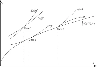
Let us summarize these results. The curve Γ = {(k, V ) | δV = u (f (k) , k)} separates the plane in two regions.
• The region below the curve corresponds to Case 0: there are no solution there.
• The region above the curve corresponds to Case 1: through each point (k∞, V∞) there are two
smooth solutions intersecting transversally. • If (k∞, V∞) is on the curve, but f
′
(k∞) + u′
2(f (k∞),k∞)
u′
1(f (k∞),k∞) ̸= δ, we are in Case 2. There are two
C1 solutions defined only on one side of k
∞. They are tangent at (k∞, V∞), and transversal
to Γ.
• If (k∞, V∞) is on the curve, and f ′
(k∞) + u′
2(f (k∞),k∞)
u′
1(f (k∞),k∞) = δ, we are in Case 3: there is a C
2
solution defined on a neighbourhood of k∞.the
Figure 1 gives the phase diagram in the (k, V ) plane:
Case 1 Case 2 Case 3 k V 1 δu(f (k), k) V1(k) V2(k) V(k) V1(k) V2(k)
Figure 1. The illustration of the solutions.
Proposition 13 gives us two solutions, Vi, i = 1, 2. Each of them gives rise to an strategy σi
through the formula σi(k) = φ0(Vi′(k) , k) with φ0 defined by (100). The strategy σi is C0 on the
half-interval, C1on its interior, with σ
i(k∞) = f (k∞).
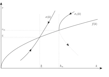
Proposition 14 One, and only one, of the strategies σ1 and σ2, converges to k∞.
Proof. Consider the Euler-Lagrange equation (16) for the Ramsey problem. The phase diagram is given in Figure 2, where k is defined by f′
(k) = δ − u′ 2/u
′ 1.
If k∞̸= k, there is one trajectory T going through (k∞, u (f (k∞) , k∞)). The point (k∞, u (f (k∞) , k∞))
separates it into two branches, the upper one and the lower one. One of them goes to (k∞, u (f (k∞) , k∞)),
and the other one leaves it. These two branches are also the trajectories associated with the two strategies σ1 and σ2, so one of them converges and the other diverges.
k k∞ k f(k) c c c∞ σ(k) σ1(k)
Figure 2. The phase diagram for the Euler equation.
Since we are looking for a strategy which converges to k∞, we pick the strategy σi, and the
solution Vi, associated with the branch oriented towards k∞. We will denote them by σ and V . We
have proved the following: Theorem 15 Suppose f′
(k∞) lies between g0(k∞) and g
0(k∞). If g
0(k∞) > g0(k∞), then there
exists an equilibrium strategy σ (k), defined on some interval ]k∞− κ, k∞] , which converges to k∞.
It is continuous on the interval, C1 on its interior, with σ (k
∞) = f (k∞). If If g
0(k∞) < g0(k∞),
there exists an equilibrium strategy with the same properties, defined on some interval [k∞, k∞+ κ[.
Note that one of the boundary values for f′
(k∞), namely g0(k∞), corresponds to the solution of
the Ramsey problem (α = 0). Indeed, the equation f′
(k∞) = g0(k∞) coincides with equation (18).
We have thus identified a class of equilibrium strategies for the Chichilnisky problem. They are one-sided, except when f′
(k∞) = g0(k∞), where we can apply Theorem 15 to get a strategy defined
on a neighbourhood of k∞. For every other value of k∞ satisfying (94) and (95), the function
V (k) and the strategy σ (k) defined by u′
1(σ (k) , k) = V ′
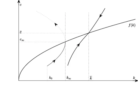
(k) are defined only on one of the two half-intervals limited by k∞. Suppose for instance it is the right one, [k∞, k∞ + κ[. Then, if
k∞≤ k0< k∞+ κ, the equilibrium strategy will bring k0 to k∞ in finite time and stay there.
To our knowledge, this is the first time equilibrium strategies have been found for the Chichilinisky criterion. Their economic interpretation, and their detailed study, will be the subject of forthcoming work.
Let us give some examples. Example 1: u (c) = U (c)
Neither depends on k, and we have:
g0(k) = δ,
g0(k) = (1 − α) δ
We have g0(k) < g0(k), so the equilibrium strategy exists only on the right hand side of g0(k).
The existence condition is:
(1 − α) δ < f′
(k∞) < δ
and the equilibrium strategy σ is defined on [k∞, ∞[. We denote f
′−1(δ) and f′−1((1 − α)δ) by k
and k respectively. There are three cases, depending on the position of the initial point k0:
• If k0 > k, then, for any k∞∈]k, k[, there exists an equilibrium strategy starting from k0 and
converging to k∞.
• if k < k0< k, then, for any k∞∈]k, k0[, there exists an equilibrium strategy starting from k0
and converging to k∞.
• if k0< k, the only equilibrium strategy starting from k0is the optimal strategy for the Ramsey
problem (that is, for the case α = 0 ) which converges to the level k where f′
(k) = δ. Example 2: u (c, k) = U (c, k) We find: g0(k) = δ − u′ 2(f (k), k) u′ 1(f (k) , k) g0(k) = (1 − α) δ − u ′ 2(f (k), k) u′ 1(f (k) , k)
The existence condition is: (1 − α) δ − u ′ 2(f (k), k) u′ 1(f (k) , k) < f′ (k∞) < δ − u′ 2(f (k), k) u′ 1(f (k) , k)
and the equilibrium strategy σ is defined on [k∞, k∞+ κ[ for some κ > 0. The situation is similar
to the preceding one, bearing in mind that now the strategy σ may be defined locally only Example 3: u = u (c) and U = U (k)
In that case, we find:
g0(k) = δ, g0(k) = δ − α (1 − α) U′ 2(f (k) , k) u′ 1(f (k) , k)
There are two subcases: • if U
′ 2(f (k),k)
u′
1(f (k),k) > 0, then g0(k) < g0(k). The equilibrium strategy then is defined on the right