HAL Id: pastel-00005622
https://pastel.archives-ouvertes.fr/pastel-00005622
Submitted on 14 Jan 2010
HAL is a multi-disciplinary open access archive for the deposit and dissemination of sci-entific research documents, whether they are pub-lished or not. The documents may come from teaching and research institutions in France or abroad, or from public or private research centers.
L’archive ouverte pluridisciplinaire HAL, est destinée au dépôt et à la diffusion de documents scientifiques de niveau recherche, publiés ou non, émanant des établissements d’enseignement et de recherche français ou étrangers, des laboratoires publics ou privés.
D’Ellsberg à Machina : les modèles de décision dans
l’ambiguïté à l’épreuve de l’expérimentation
Laetitia Placido
To cite this version:
Laetitia Placido. D’Ellsberg à Machina : les modèles de décision dans l’ambiguïté à l’épreuve de l’expérimentation. Sciences de l’Homme et Société. HEC PARIS, 2009. Français. �pastel-00005622�
ECOLE DES HAUTES ETUDES COMMERCIALES DE PARIS
Ecole Doctorale « Sciences de la Décision et de l’Organisation » - ED 471
Equipe de Recherche GREGHEC - UMR 2959
« From Ellsberg to Machina:
Confronting decision models under ambiguity with experimental evidence »
THESE
présentée et soutenue publiquement le 23 juin 2009
en vue de l’obtention du
DOCTORAT EN SCIENCES DE GESTION
par
Lætitia PLACIDO
JURY
Président du jury : Monsieur Chris STARMERProfesseur
University of Nottingham – Royaume Uni
Directeur de recherche : Monsieur Mohammed ABDELLAOUI
Directeur de recherche CNRS, Professeur Affilié Ecole des Hautes Etudes Commerciales
Rapporteurs : Monsieur Jean-Marc TALLON
Directeur de recherche CNRS, Professeur Associé
Ecole d’Economie de Paris, Université de Paris 1 Panthéon Sorbonne
Monsieur Peter P. WAKKER
Professeur
Erasmus University, Rotterdam – Pays-Bas
Suffragants : Monsieur Bertrand MUNIER
Professeur des Universités
Institut d’Administration des Entreprises – Paris 1 Panthéon Sorbonne
Monsieur Stéphane SAUSSIER
Professeur des Universités
Institut d’Administration des Entreprises – Paris 1 Panthéon Sorbonne
Monsieur Marc VANHUELE
Ecole des Hautes Etudes Commerciales
Le Groupe HEC Paris n’entend donner aucune approbation ni improbation aux
opinions émises dans les thèses ; ces opinions doivent être considérées
Remerciements - Acknowledgements
De nombreuses personnes ont contribué de près ou de loin à l’élaboration de cette thèse. Ces remer-ciements leur sont adressés.
Je tiens à remercier en tout premier lieu mon directeur de thèse, Mohammed Abdellaoui, pour m’avoir acceptée en tant que doctorante et pour la confiance et la liberté qu’il m’a accordées tout au long de cette thèse. Ses conseils avisés dans l’orientation de mon travail ont été et seront les moteurs indispensables à l’avancement de mes recherches.
Je remercie également les professeurs Jean-Marc Tallon et Peter Wakker d’avoir accepté d’être les rapporteurs de cette thèse et d’en avoir commenté les versions préliminaires, ainsi que les professeurs Bertrand Munier, Stéphane Saussier, Chris Starmer et Marc Vanhuele d’avoir accepté de faire partie de mon jury.
Je tiens à remercier tout particulièrement Aurélien Baillon pour sa très grande disponibilité, son en-thousiasme permanent et son regard critique qui m’ont permis d’avancer dans les moments décisifs de cette thèse. Les débats, parfois houleux, autour de nos sujets de recherche ont fait naître une franche amitié.
Mes remerciements reviennent également à :
Michèle Cohen pour m’avoir fait découvrir la théorie de la décision et m’avoir encouragée à pour-suivre dans cette voie ;
Peter Klibanoff pour sa patience et sa bienveillance. Travailler à ses côtés est une expérience des plus enrichissantes ;
Mark Machina dont les commentaires ont été d’un grand apport pour cette thèse ;
Olivier L’Haridon et Brian Hill qui resteront, je l’espère, de solides compagnons de route ;
Lionel Page, Corina Paraschiv, Cédric Paternotte, Kirsten Rohde et Horst Zank pour toutes les discus-sions stimulantes que nous avons eues ;
Nathalie Etchart, Catherine MacMillan et Aurélie Martin pour m’avoir apporté leur soutien dans les dernières étapes de cette thèse ;
Bertrand Munier, directeur du GRID, pour m’y avoir accueillie et donné les conditions de travail idéales pour le commencement de cette thèse ainsi qu’à toute l’équipe du GRID, en particulier Nicolas Drouhin pour avoir été à l’écoute depuis le début et pour les injections de confiance qu’il m’a prodiguées quand il le fallait ;
Marc Vanhuele, directeur du GREGHEC, ainsi que Philippe Mongin pour s’être souciés de ma bonne installation au sein du laboratoire et pour avoir fait en sorte que ma thèse puisse se terminer dans les meilleures dispositions ; Nathalie Beauchamp pour sa constante bonne humeur et son efficacité red-outable ; Antoine et Emmanuel pour avoir contribué à créer un environnement studieux et agréable.
Enfin, je remercie ma grand-mère, ma mère, mon père, Leïa, Indy et Gautier pour qui la vision obscure de la théorie de la décision n’a pas empêché un soutien au quotidien et une aide précieuse.
Table of contents
Introduction 9
Choice under uncertainty . . . 9
Contribution and outline of the thesis . . . 9
I Subjective Uncertainty: Models and Paradoxes 17 1 Modeling Subjective Uncertainty 18 1.1 Introduction . . . 18
1.2 Savage’s approach . . . 19
1.2.1 Framework and notations . . . 19
The state space . . . 19
The outcome space . . . 22
The choice space . . . 22
1.2.2 Savage’s axiomatization . . . 23
1.3 Anscombe-Aumann’s approach . . . 26
1.3.1 Framework and notations . . . 26
1.3.2 Anscombe-Aumann’s axiomatization . . . 26
1.4 Probabilistic sophistication . . . 28
1.4.2 Chew and Sagi’s PS . . . 29
1.5 Ellsberg paradox . . . 30
1.5.1 Two-urn experiment . . . 30
1.5.2 One-urn experiment . . . 31
1.6 The modeling of ambiguity . . . 32
1.6.1 Choquet expected utility . . . 32
1.6.2 Multiple Prior models . . . 34
Maxmin expected utility . . . 34
α-MEU . . . 37
Variational preferences . . . 39
Ambiguity as imprecise information . . . 40
Ambiguity and indecision . . . 41
Others approaches . . . 43
Limitations . . . 43
1.6.3 Multiple Stage models . . . 44
Klibanoff, Marinacci and Mukerji (2005) . . . 44
Seo (2008) . . . 45
Halevy & Ozdenoren (2008) . . . 45
Ergin & Gul (2009) . . . 46
1.6.4 Sources of uncertainty . . . 46
Epstein and Zhang (2001) . . . 46
Source dependence and small worlds . . . 47
2 Sources of Uncertainty and Ambiguity Attitudes 52 2.1 Introduction . . . 52
Bringing ambiguity attitudes to light through separate sources of
uncer-tainty . . . 54
. . . and playing with them via mixed sources of uncertainty . . . 55
Notations . . . 56
2.2 Separate sources of uncertainty . . . 56
2.2.1 Ellsberg two-urn paradox . . . 56
2.2.2 Common interpretations . . . 59
Interpretation in terms of missing information . . . 59
Interpretation in terms of a two-stage representation of uncertainty . . . 60
Uniform sources interpretation . . . 62
2.2.3 Psychological causes of ambiguity aversion . . . 64
Social factors . . . 64
Framing effects . . . 66
2.3 Mixed sources of uncertainty . . . 67
2.3.1 Ellsberg one-urn paradox . . . 68
The second-order uncertainty aversion interpretation . . . 70
Separating sources in mix decision problems . . . 71
2.3.2 The reflection paradox . . . 75
2.4 Conclusion . . . 77
II Ellsberg Paradox: Two Experimental Approaches 83 3 The Source of Uncertainty Approach 84 3.1 Introduction . . . 85
3.2 Framework . . . 87
3.2.2 Ellsberg paradox . . . 87
3.2.3 A general biseparable model . . . 88
3.2.4 Probabilistic sophistication . . . 89
3.2.5 Source functions . . . 89
3.2.6 A focus on source functions . . . 90
3.3 Experiment . . . 93
3.3.1 Experimental design . . . 93
Participants . . . 93
Two decision contexts . . . 93
Measuring indifferences . . . 93
Order treatments . . . 94
Incentive mechanism . . . 95
3.3.2 Elicitation technique . . . 95
Testing exchangeability . . . 95
Elicitation of the utility function . . . 96
Decision weights . . . 96
Parametric fitting of the source functions . . . 96
Indexes . . . 97
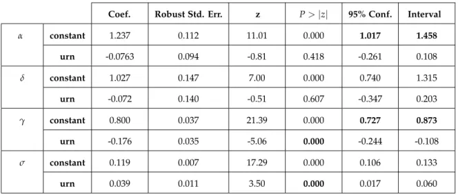
3.4 Results . . . 97
3.4.1 Exchangeability . . . 97
3.4.2 Utility . . . 99
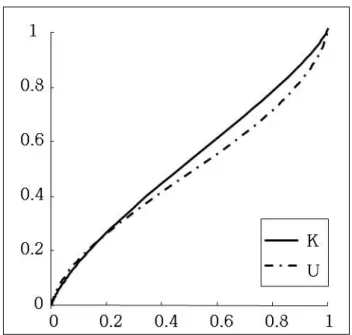
3.4.3 Sources functions . . . 99
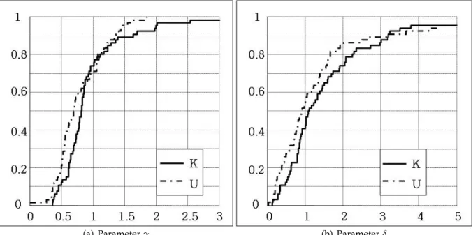
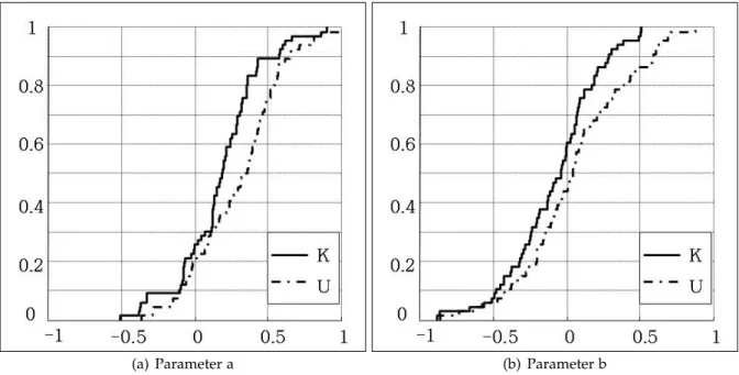
3.4.4 Parametric fitting of source functions . . . 101
3.4.5 Indexes . . . 103
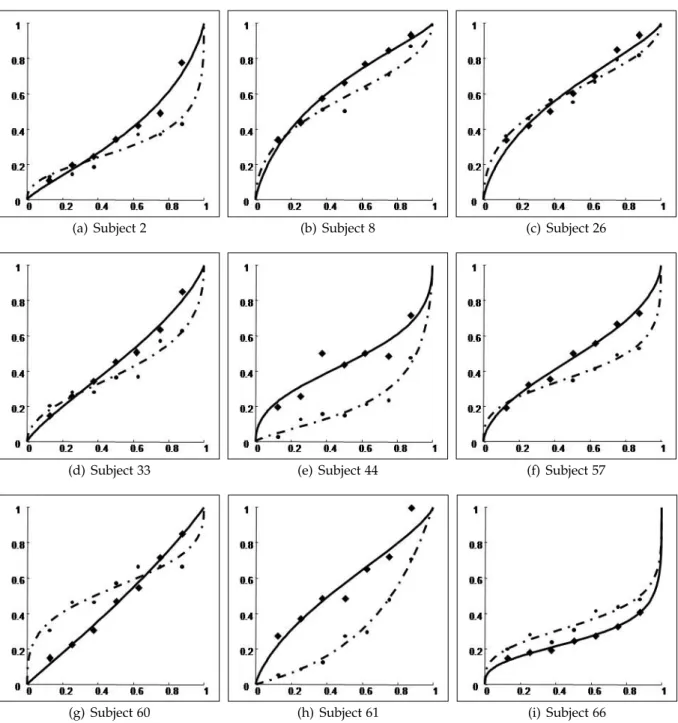
3.4.6 Heterogeneity . . . 104
3.5 Discussion and further results . . . 106
3.5.1 Qualitative features and statistical methods . . . 106
3.5.2 Order effects and the comparative ignorance hypothesis . . . 107
3.5.3 Ambiguity and asset prices . . . 108
3.5.4 Sources of uncertainty . . . 110
3.5.5 Ellsberg one-urn paradox . . . 110
3.5.6 Conclusion . . . 111
4 The Compound Risk Approach 120 4.1 Introduction . . . 121
4.2 Experiment . . . 123
4.2.1 Uncertainties . . . 123
4.2.2 Mechanisms to create ambiguity . . . 124
4.2.3 Sample . . . 125
4.2.4 Procedure . . . 125
4.2.5 Incentives . . . 127
4.3 Results . . . 128
4.3.1 Failures in reduction of compound lotteries . . . 128
Time neutrality . . . 129
Reduction and likelihood treatments . . . 129
Individual level . . . 130
Simple risk and mean compound risk . . . 131
4.3.2 Exchangeability . . . 131
4.4 Attitude towards ambiguity and attitude towards compound risk . . . 132
4.4.2 Regressions . . . 135
4.4.3 The impact of likelihood on attitudes towards ambiguity, risk and com-pound risk . . . 136
4.5 Summary and conclusion . . . 139
III Machina Paradox: A Challenge for Ambiguity Models? 147 5 Machina Paradox and CEU: An Empirical Evidence 148 5.1 Introduction . . . 149
5.2 Framework . . . 154
5.2.1 Subjective expected utility . . . 154
5.2.2 Choquet expected utility . . . 155
5.2.3 The reflection example . . . 157
5.2.4 Proper criteria to analyze ambiguity . . . 161
Individual payoffs . . . 162
Decumulative payoff events . . . 162
Exposure to ambiguity . . . 163
5.3 Experiment . . . 164
5.4 Results . . . 165
5.4.1 Confirming Ellsberg paradox . . . 165
5.4.2 Informational symmetry . . . 166
5.4.3 A paradox for Choquet expected utility . . . 167
5.4.4 An empirically-consistent approach for ambiguity . . . 167
5.4.5 Other effects . . . 168
5.5 Discussion . . . 168
5.5.1 Choquet expected utility versus informational symmetry? . . . 168
5.5.2 Informational symmetry and editing . . . 170
5.5.3 Quality of the CEU model . . . 171
6 An Allais-like Paradox for Generalized Expected Utility Theories ? 181 6.1 Introduction . . . 182
6.2 Framework of the experiment . . . 184
6.2.1 Rank-dependent expected utility . . . 184
6.2.2 Allais-like choices . . . 186
6.2.3 Experiment . . . 187
6.3 Results . . . 188
6.4 Conclusion . . . 189
7 Machina Paradox’s Collateral Damages for Ambiguity 192 7.1 Introduction . . . 193
7.2 Four popular models of ambiguity-averse preferences . . . 193
7.3 The 50:51 example . . . 196
7.4 The reflection example . . . 199
7.4.1 Decision criteria and experimental results . . . 200
7.4.2 Confrontation of the four models with the reflection example . . . 202
7.5 The implications of Machina’s examples for other models . . . 204
7.6 Conclusion . . . 205
Discussion 213 Are ambiguity attitudes rational? . . . 213
Introduction
Choice under uncertainty
Knight (1921) first introduced the distinction between measurable uncertainty, in which
prob-abilities are known; and non measurable uncertainty, in which they are unknown. In both
cases, a decision maker has to choose between uncertain alternatives, whose consequences
depend on events that can possibly occur. The decision maker endorses a preference relation
over all the available actions. The normative principle of decision theory is that the decision
maker ought to undertake the best action with respect to his preferences. The model used to
predict the behavior will depend on the informational context confronting the decision maker
and account for the decision maker’s attitude given this context.
The benchmark of decision making under uncertainty is the case of risk. All the events
under consideration can be associated with objective probabilities and the decision maker
typically applies expected utility theory (von Neumann and Morgenstern, 1944). Allais (1953)
shook the predictive power of the theory by pointing out its descriptive limitations in the
presence of the certainty effect. Savage (1954) extended (objective) expected utility to
infor-mational contexts where the decision maker has no objective probabilistic information at his
disposal. Subjective expected utility assumes that the decision maker assigns subjective
ad-ditive probability on events. Then, the decision maker computes the expected utility of each
action with respect to his subjective probability and chooses the action associated with the
INTRODUCTION
higher subjective expected utility. If the decision maker more generally behaves in a way
that can be analyzed in terms of probabilities without necessarily conforming to the expected
utility rule, then he is defined as probabilistically sophisticated (Machina and Schmeidler,
1992). However, an underlying condition of models that are based on subjective probability is
that the decision maker effectively treats subjective probabilities as if he is dealing with
objec-tive probabilities, independent of the amount of information that leads to the formulation of
the personal probability. This condition is far from being respected for some specific choice
problems, notably those involving ambiguity.
Ambiguity defines decision contexts where no probabilities are available to (nor can be
subjectively revealed by) the decision maker to take one’s decision. Ellsberg (1961) proposed
thought experiments suggesting that the presence of ambiguity in decision making may affect
behavior in a way that deviates from subjective expected utility. He suggested that most
peo-ple prefer to bet on the color of a ball drawn from a risky urn with known composition (fifty
red, fifty black), rather than on the color of a ball drawn from a similar urn containing 100
balls with an unspecified composition. This behavior reveals that the probability of drawing
a red (or equivalently black) ball in the unspecified urn is less than one-half. Such a decision
maker violates subjective probabilities and (ex ante) probabilistic sophistication which predict
that the probabilities of drawing a red or a black ball should sum to one. Ellsberg concluded
that decision makers tend to avoid ambiguity, exhibiting what he termed ambiguity aversion.
Subsequently, a large experimental literature has empirically confirmed Ellsberg’s
con-tradicting examples, and a large theoretical literature has developed alternative models to
accommodate non neutral attitudes towards ambiguity. A pioneer approach generalizes
sub-jective expected utility to non additive probability measures (Schmeidler, 1989; Gilboa, 1987;
Tversky and Kahneman, 1992). The multiple prior approach (Gilboa and Schmeidler, 1989;
INTRODUCTION
measures. In a final two-stage approach, a decision maker formulates subjective beliefs (first
stage) over probability distributions (second stage) but does not necessarily reduce the two
stages (Klibanoff, Marinacci and Mukerji, 2005; Seo, 2008; Halevy and Ozdenoren, 2008).
All these models provided successful predictions of the behavior under ambiguity until a
recent contribution from Machina (2009). Machina proposed a slight modification of the
Al-lais1and Ellsberg examples and predicted that the plausible preferences cannot be explained by the most popular models accounting for these paradoxes, i.e., rank-dependent utility under
risk (Quiggin, 1982) and Choquet expected utility for ambiguity (Schmeidler, 1989).
The object of this thesis is to describe and analyze individual decision making in the
context of ambiguity. It is based on both Ellsberg and Machina paradoxes and mainly adopts
the experimental approach.
Contribution and outline of the thesis
This thesis aims to provide new insights to the understanding of decision behavior under
ambiguity. It is composed of three parts.
The first part is a survey of the literature on ambiguity. Chapter 1 presents the
model-ing of subjective uncertainty and ambiguity. Chapter 2 envisages ambiguity attitudes as a
consequence of the joint presence of objective and subjective sources of uncertainty.
The second part explores two specific approaches to the Ellsberg paradox. Different
mod-els might be appropriate in describing the individual behavior towards ambiguity, the
di-versity of approaches reflecting the heterogeneity of human cognitive processes. A common
feature of the approaches adopted here is that they allow one to analyze attitudes towards
ambiguity as likelihood-dependent. Chapter 3 reconciles ambiguity attitudes with
probabilis-tic sophisprobabilis-tication in the Ellsberg two-urn problem. Ambiguity is viewed as a specific source of
INTRODUCTION
uncertainty (notably as opposed to risk). The method employs Chew and Sagi’s (2006, 2008)
exchangeability concept to define probabilistic sophistication within a source of uncertainty
while not requiring it between sources. It provides a quantitative measurement of behavior
through source functions, one for the risky urn and one for the ambiguous urn. The shapes
of these functions are found to be different, which empirically confirms the soundness of
ap-proaches based on sources of uncertainty (Tversky and Wakker, 1995), and at the same time,
reconciles non neutral attitudes towards ambiguity with probabilistic sophistication on
con-dition that exchangeability holds within each source of uncertainty. Chapter 4 adopts a quite
different, and perhaps, not contradictory perspective. It studies the idea that decision makers
assimilate ambiguity to compound risk. It further investigates a recent empirical finding that
establishes equivalence between reduction of compound lotteries and ambiguity neutrality
(Halevy, 2007). Our data confirm a link between ambiguity attitudes and compound risk
attitudes. However, it puts into perspective Halevy’s conclusion, since the equivalence does
not match the data: decision makers who fail to reduce compound lotteries are non neutral
to ambiguity but those who reduce compound lotteries are not necessarily ambiguity neutral
and are even prone to ambiguity aversion. This result does not support recent axiomatizations
(Halevy and Ozdenoren, 2008; Seo, 2008) that explicitly relate compound risk and ambiguity.
The third part is entirely based on a recent contribution by Mark Machina (2009). Machina
considers a slight modification of the Ellsberg original one-urn problem and convincingly
proves that the pattern of preferences that could emerge from his construction is not
compat-ible with Choquet expected utility (Schmeidler, 1989). Chapter 5 provides empirical evidence
for the thought experiment proposed by Machina and confirms the possibility of extending
the Ellsberg paradox to one of the major models that accounts for ambiguity aversion, i.e,
Choquet expected utility. At the same time, Chapter 6 empirically undermines such an
INTRODUCTION
Chapter 7, which is theoretical, it is proved that the conclusions of Machina are not restricted
to Choquet expected utility but can be extended to four other prominent models of ambiguity
as well. Notably, the class of models with sets of priors - including, Gilboa and Schmeidler’s
maxmin expected utility (1989), its extensions, α-maxmin expected utility and the variational
preferences - and the smooth model of ambiguity aversion (Klibanoff, Marinacci and Mukerji,
2005) are also contradicted by Machina’s paradox.
All chapters except those in Part 1 are self-contained in the sense that they are readable
independently. Consequently, notations and concepts may appear several times.
The experimental or theoretical results incorporated in this thesis correspond to the
fol-lowing research papers: Chapter 4 refers to a subpart of Abdellaoui, Baillon, Placido and
Wakker (2009a), Chapter 5 to Abdellaoui, Klibanoff and Placido (2009b), Chapter 6 and 7 to
Bibliography
Abdellaoui, M., Baillon, A., Placido, L., & Wakker, P. P. (2009a). The rich domain of
uncer-tainty: Source functions and their experimental implementation. Working paper.
Abdellaoui, M., Klibanoff, P., & Placido, L. (2009b). Ambiguity and reduction of compound
lotteries. Working paper.
Allais, M. (1953). Le comportement de l’homme rationnel devant le risque: critique des
postulats et axiomes de l’école américaine. Econometrica, 21, 503–546.
Baillon, A., L’Haridon, O., & Placido, L. (2009). Risk, ambiguity, and the rank-dependence
axioms: Comments. Working paper, HEC-Paris School of Management.
Chew, S. H., & Sagi, J. S. (2006). Event exchangeability: Probabilistic sophistication without
continuity or monotonicity. Econometrica, 74, 771–786.
Chew, S. H., & Sagi, J. S. (2008). Small worlds: Modeling attitudes toward sources of
uncer-tainty. Journal of Economic Theory, 139(1), 1–24.
Ellsberg, D. (1961). Risk, ambiguity and the Savage axioms. Quarterly Journal of Economics, 75,
643–669.
Ghirardato, P., Maccheroni, F., & Marinacci, M. (2004). Differentiating ambiguity and
BIBLIOGRAPHY
Gilboa, I. (1987). Expected utility with purely subjective non-additive probabilities. Journal of
Mathematical Economics, 16(1), 65–88.
Gilboa, I., & Schmeidler, D. (1989). Maxmin expected utility with non-unique prior. Journal of
Mathematical Economics, 18(2), 141–153.
Halevy, Y. (2007). Ellsberg revisited: An experimental study. Econometrica, 75(2), 503–536.
Halevy, Y., & Ozdenoren, E. (2008). Uncertainty and compound lotteries: Calibration. Working
paper, University of British Columbia.
Klibanoff, P., Marinacci, M., & Mukerji, S. (2005). A smooth model of decision making under
ambiguity. Econometrica, 73(6), 1849–1892.
Knight, F. H. (1921). Risk, Uncertainty, and Profit. Boston, MA: Houghton Mifflin Co.
L’Haridon, O., & Placido, L. (2008). An Allais paradox for generalized expected utility
theo-ries? Economic Bulletin, 4(19), 1–6.
L’Haridon, O., & Placido, L. (2009). Betting on Machina’s reflection example: An experiment
on ambiguity. forthcoming in Theory and Decision.
Machina, M. (2009). Risk, ambiguity, and the rank-dependence axioms. American Economic
Review, 99(1), 385–392.
Machina, M. J., & Schmeidler, D. (1992). A more robust definition of subjective probability.
Econometrica, 60(4), 745–80.
Quiggin, J. (1982). A theory of anticipated utility. Journal of Economic Behavior & Organization,
3(4), 323–343.
BIBLIOGRAPHY
Schmeidler, D. (1989). Subjective probability and expected utility without additivity.
Econo-metrica, 57, 571–587.
Seo, K. (2008). Ambiguity and second order belief. forthcoming in Econometrica.
Tversky, A., & Kahneman, D. (1992). Advances in prospect theory: Cumulative representation
of uncertainty. Journal of Risk and Uncertainty, 5, 297–323.
Tversky, A., & Wakker, P. P. (1995). Risk attitudes and decision weights. Econometrica, 63,
1255–1280.
von Neumann, J., & Morgenstern, O. (1944). Theory of Games and Economic Behavior. Princeton
Part I
Subjective Uncertainty: Models and
Paradoxes
Chapter 1
Modeling Subjective Uncertainty
1.1
Introduction
Standard economic modeling describes behavior under uncertainty by making the
assump-tion that a decision maker (henceforth, DM) always has either an objective probability at his
disposal (Von Neumann and Morgenstern: vNM, 1944) or can formulate subjective additive
probability (Savage, 1954) in any decision context. In both cases, the DM is assumed to
com-pute the expected utility of each possible decision with respect to the objective/subjective
probability and choose the decision associated with the highest objective/subjective expected
utility. However, Ellsberg (1961) remarks that such a rule no longer applies in a specific
de-cision context called ambiguity. This chapter aims at giving an overview of the literature on
subjective uncertainty including subjective expected utility and its generalizations to
ambigu-ity.
Section 1.2 presents the modeling of subjective uncertainty introduced by Savage (1954)
who first gave all the ingredients for obtaining a purely subjective decision model. Indeed,
both tastes given by the utility function and beliefs given by the probability measure
1.2. SAVAGE’S APPROACH
over decisions. Section 1.3 describes the approach of Anscombe and Aumann (1963), which
reintroduces some objective elements to make the axiomatization closer to expected utility
for risk. Section 1.4 presents generalizations of subjective uncertainty based on probabilistic
sophistication. Section 1.5 focuses on ambiguity attitudes as a contradiction of the classic
modeling of subjective uncertainty (Ellsberg, 1961). Eventually, Section 1.6 presents models
that have been developed to take into account non neutral ambiguity attitudes.
1.2
Savage’s approach
Savage’s (1954) subjective expected utility (SEU) consists of an extension of vNM expected
utility to decision context where objective probabilities are not available. It provides a set of
technical and behavioral axioms that are sufficient to characterize both a utility function and
a probability measure. Because both are derived from conditions on preferences, the theory
is said to be fully subjective.
1.2.1 Framework and notations
Savage’s formulation is based on three elements: the state space that modelizes uncertainty,
the set of outcomes that describes the possible consequences a DM can undergo, and the set
of acts that relates the two, and on which the DM has a preference relation.
The state space
The state space (or the world) S is "the object about which the person is concerned” and
contains the states of the world. We assume S finite. A state of the world s is an element of S
and is "a description of the world, leaving no relevant aspect undescribed”. The resolution
of uncertainty relies on the properties of the states of the world: (i) exhaustive: a DM is able
1.2. SAVAGE’S APPROACH
exclusive: two distinct states cannot simultaneously occur, (iii) only one state is true: "the state
that does in fact obtain” (Savage, p. 9).
Events Ei are subsets of S, and 2S is the set of all the subsets of S. The universal event S
is the event having every state of the world as element. The vacuous event∅ has no state as element. A collection of events {E1, . . . , En} with n belonging to the natural number, forms a
partition of the state space.
Conceptual and descriptive limitations. The main limitations of Savage’s state space are due to the assumption of exogeneity that bears on it.
First, each state represents nature’s exogenous uncertainty. This implies that it should
be possible to reconstruct on the basis of a DM’s observed choices, the unique state space
underlying his decisions. However, as argued by Machina (2003), there is no guarantee that
the state space thus obtained corresponds to the state space that preexists and is observed, or
to an endogenous construction of the DM.
Second, the exhaustivity requirement imposes that the DM have a complete representation
of the word. As shown by Newcomb’s paradox (see Gilboa, 2003), evidence can lead the DM
to conclude that his initial image of the world is incomplete. More concretely, the exhaustivity
of the state space seems impossible to guarantee in practice due to objective complexity and
human cognitive limitation. As pointed out by Karni (2006): "the depiction of the relevant
state space is often unintuitive and too complex to be compatible with DMs’ perception of
choice problems”.
Third, exogeneity implicitly supposes that the DM is aware of all the states that can occur.
Consequently, the state space leaves no room for unforeseen contingencies, and at best "when
the DM has reason to ’expect the unexpected’ (. . . ) the best one can do is specify a final,
catch-all state, with a label like ’none of the above’, and a very ill-defined consequence” (Machina,
1.2. SAVAGE’S APPROACH
Finally, exogeneity can be conceptually called into question for a theory that claims to
be subjectivist. Epstein and Zhang (2001) argue that a fully subjective theory should derive
both the domain and the subjective probability from preferences. They tend to remedy this
conceptual limitation by proposing an axiomatization that endogenously defines a domain on
which a DM has subjective probabilities from the rest of the world on which the DM ought
not to have such probabilities.
The two following remarks express more descriptive concerns since they point out
behav-ioral assumptions contained in Savage’s axioms. The realization of the state is independent
of the action undertaken by the DM. As argued by Karni (2006), this assumption seems
un-realistic and implies unconceivable fatalism. Eventually, the evaluation of a consequence is
independent on the state in which it is received (the utility is state independent).
These remarks reveal Savage’s construction to be conceptually limited and descriptively
inadequate for the representation of many decision problems. The literature provides some
extensions that aim to remedy to such limitations.
Extensions. Extensions have been provided that allow for a more flexible and realistic description of the world. Indeed, a DM facing a decision problem is generally not provided
with the background structure.
Ghirardato (2001) envisages that events which are relevant for the result of the DM’s
choices may have been left out of the description of the state space and refers to ’unforeseen
contingencies’. The DM is aware of his ignorance and perceives the state space as
under-specified; this is formally represented by correspondences: each state s under consideration
is a collection of possible states, differing in aspects which have not been included in the
description of s.
In Dekel, Lipman and Rustichini (2001), the state space reflects the DM’s subjective
1.2. SAVAGE’S APPROACH
his endogenously defined subjective state space.
Karni (2006) proposes a theory that dispenses with the state space and accommodates
both the presence of moral hazard considerations as well as the possibility that the evaluation
of the consequences of decisions are effect-dependent. He obtains subjective expected utility
with unique and action-dependent subjective probability.
Chew and Sagi (2008) points out that, although Savage envisaged a big world as defined
above, he, at the same time observed that decisions are generally made in smaller worlds,
which contain events summarizing the relevant aspects of the contingencies pertaining to
specific decision situations. In Savage ’s formulation, events in any small world are
compara-ble to events in any other small world and they all remain similar to the big world. Hence,
Savage implicitly assumes that the DM’s attitude is independent of the small world in which
the decision is taken. Chew and Sagi refine Savage’s small world approach, basing it on the
intuition of similarity among events. They introduce the concept of small world events domain
defined as a collection of comparable events; they provide consistency conditions that explain
the presence of distinct attitudes between small worlds.
The outcome space
To each event that occurs there follows a consequence, i.e., "anything that may happen to the
person”. The set of consequences X is finite and will refer to monetary outcomes, although
Savage defines more generally the "states of the person".
The choice space
Objects of choice are called acts. The set of acts isA = {f : S→ X}, i.e., maps from the state
space to the outcome space. f(s)represents the consequence of choosing f if the state of the
1.2. SAVAGE’S APPROACH
otherwise. A constant act gives the same outcome over all the states the world ( f(s) = x
f or all s ∈ S) and is shortly designated by the unique outcome x it is associated with. We
assume that acts have only finite consequences. Hence, an act will be alternatively written[x1
on E1; . . . ; xn on En] with the understanding that xi is obtained if Ei is true. The DM has a
preference relation%over A. %denotes weak preference with and∼the strict preference
and indifference, respectively (-denote the reverse preference).
E is a null event if indifference holds between all pairs of acts that only differ on E:
Definition 1(Null event). E⊆ S is a null event if for all f , g, h∈ A,
[f on E; h on non E] ∼ [g on E; h on non E].
Null events will turn to be those with zero probability.
1.2.2 Savage’s axiomatization
Savage provides a set of postulates for preference among acts. According to Savage, a rational
DM ought to satisfy these postulates and he shows that conforming to these postulates is
equivalent to agreeing with a ranking of acts in term of subjective expected utility.
P 1 (Ordering)The preference relation%is a weak order (complete and transitive) P1 says that preferences should be transitive: if a DM prefers act f to act g, and act g
to act h, then he should prefer act f to act h. The transitivity condition is itself normatively
desirable and not controversial as a rationality requirement. However, as argued by Shafer
(1986), Savage goes one step further by making the assumption of completeness, that imposes
a DM should always have well-defined preferences between acts f , g and h. Imagine a DM
who actually does not have preferences between these particular three acts, in words, he is
indecisive; it comes from Savage’s P1 that the DM is obliged to construct these preferences.
Moreover, even if they exist, preferences are often unstable and non robust to procedural
1.2. SAVAGE’S APPROACH
"When faced with a choice among several alternatives, people often experience
uncertainty and exhibit inconsistency. That is, people are often not sure which
alternative they should select, nor do they always make the same choice under
seemingly identical conditions.”
The three following axioms provide together the disentanglement between subjective
probabilities and the subjective values of consequences (utilities).
P 2 (Sure-thing principle) for all events E and for all acts f , g, h, h∗ ∈ A,
[f on E; h on non E] % [g on E; h on non E] ⇒ [ f on E; h∗on non E] % [g on E; h∗ on non E]
P2 says that if two acts are equal on a given event non E, then the preference ranking over
these acts should not depend on what they are equal to on non E. In words, the DM does not
care about what is sure, h or h∗, when choosing between f and g. Intuitively, this condition
implies that preferences are separable on mutually exclusive events. The sure-thing principle
constitutes the weak point of Savage’s theory and is violated as soon as DMs exhibit non
neutral ambiguity attitudes (see Chapter 2).
P 3 (Eventwise monotonicity) for all act f ∈ A, for all outcomes x, y∈X, for all non null event E,[x on E; f on non E] % [y on E; f on non E] ⇔x%y
The DM who weakly prefers the sure consequence x to the sure consequence y will choose
the right act because the alternative yields less on the event on which the acts differ. This
axiom implies that the tastes concerning outcomes do not depend on the events under which
they are received. Hence, utility is not state dependent.
P 4 (Weak comparative probability)for all events E, F and outcomes x y and x0 y0,
[x on E; y on non E] % [x on F; y on non F] ⇒ [x0 on E; y0 on non E] % [x0 on F; y0on non F]
P4 says that, since x is more desirable than y, the first act is a win if E occurs and the
second is a win if F occurs. The first is weakly preferred to the second if event E is judged at
1.2. SAVAGE’S APPROACH
desirable than y0. In brief, beliefs on events do not depend on the consequences. P3 adds
that this ranking in term of likelihood does not depend on the consequences used. Thus, P4
allows to infer an ordering of events in terms of likelihood and is then crucial for the existence
of subjective probabilities.
P 5 (Non degeneracy)∃two outcomes x, y∈ X such that x y
P5 guarantees the existence of the probability measure. If this axiom is not true (∀x, y∈
X, x∼ y), the DM is indifferent to all consequences so there is no longer a decision problem.
Note that it also means that S is not a null event.
P 6 (Small event continuity) For any acts f g and outcome x ∈ X there exists a finite set of events{E1, . . . , En}partitioning S such that ∀i∈ {1, . . . , n}:
f [x on Ei; g on non Ei]and[x on Ei; f on non Ei] g
P6 implies that S can be partionned in sufficiently small events so that a modification
of each act (by putting the best or the worst outcome on one of these small events) is not
sufficient for reversing the original preference order.
Theorem 1 (Savage, 1954). Under P1-P6 there exists a unique finitely additive and non atomic probability measure P(.)on 2Sand a state-independent utility function u(.) on the set of outcomes X
such that the subjective expected value of act f is:
SEU(f) =
∑
s∈S
P(s)u(f(s)) (1.1)
Moreover, u(.) is unique up to a positive linear transformation.
Act f is preferred to another act g if the expected utility calculated with respect to the
subjective probability measure P is higher for f than for g. The subjective measure P is
derived from the preference of the DM and is thus personal. Consequently, two DMs might
1.3. ANSCOMBE-AUMANN’S APPROACH
1.3
Anscombe-Aumann’s approach
Anscombe and Aumann (1963) propose an alternative derivation of SEU. An act f is a map
from the state space to the set of lotteries over consequences (and no longer to the set of
consequences as in Savage).
1.3.1 Framework and notations
The preference relation%is defined on the set of actsF = {f : S→ L}, whereLis the set of
simple lotteries (with finite support) on X. An element ofLis a lottery l= (x1, p1; . . . ; xn, pn)
which gives the consequences xi with probability pi. Hence, each act f inF combines "horse
race lotteries” (i.e., Savagean acts) and "roulette lotteries” (i.e., objective lotteries) and can be
written in the following way[. . . ;(. . . ; xi, pi; . . . ) on Ej; . . .]. f can be interpreted as a bet on
a horse race, but instead of receiving the winnings of the bet directly in money, the DM is
actually given a ticket for a lottery with objective probabilities.
The λ-mixture of acts f = (l1, . . . , ln)and g = (l10, . . . , ln0)with λ ∈ [0, 1] noted λ f + (1− λ)g yields λ f(i) + (1−λ)g(i) = λli+ (1−λ)li0 on state i. Thanks to mixture,
Anscombe-Aumann’s axiomatization will be very similar to vNM’s.
1.3.2 Anscombe-Aumann’s axiomatization
A 1 (Weak order)The preference relation% is a weak order (transitive and complete) Bewley (2002) proposes a theory of choice under subjective uncertainty that removes the
completeness axiom from the Anscombe-Aumann setting but he needs to introduce an inertia
assumption to deliver a representation theorem.
A 2 (Independence) for all f , g, h∈ F, and for all λ∈ [0, 1], f %g⇒λ f + (1−λ)h%λg+ (1−λ)h
1.3. ANSCOMBE-AUMANN’S APPROACH
A 3 (Jensen continuity) for all f , g, h∈ F, if f g h, then∃λ, µ∈]0, 1[such that,
λ f + (1−λ)h g µ f+ (1−µ)h
The lottery is only played after a particular state s ∈ S occurs; hence, axioms A1-A3
only deliver a state-dependent expected utility function Us : L →X and the preferences are
represented by:
A(f) =∑s∈SUs(ls)
Intuitively, for obtaining state independent expected utility we need something that says
that a preference between two lotteries l and l0has to be preserved whatever the state is. First
we need to introduce one definition:
Definition 2(Null state). s∈ S is a null state if for all q, q0 ∈ L (l1, . . . , ls−1, q, ls+1, . . . , ln) ∼ (l10, . . . , ls0−1, q0, l0s+1, . . . , l0n).
If a DM is indifferent between these two acts, then effectively state s does not matter, i.e.
it is equivalent to stating that the DM believes s will never happen. It will be assumed that
there are at least some states that are non-null states. To establish this, the following axiom is
needed:
A 4 (Non degeneracy) ∃f , g∈ F such that f g A4 guarantees the existence of non-null states.
A 5 (State independence)s∈S is a non-null state and q, q0 ∈ L. If
(l1, . . . , ls−1, q, ls+1, . . . , ln) (l10, . . . , ls0−1, q0, l0s+1, . . . , l0n)then, for every non-null state t∈ S,
(l1, . . . , lt−1, q, lt+1, . . . , ln) (l10, . . . , l0t−1, q0, l0t+1, . . . , ln0)
Theorem 2(Anscombe-Aumann, 1963). Under A1 - A5 there exists of a unique probability measure P(.) on S and a state-independent expected utility function U(.) on L such that act f is evaluated
through:
AA(f) =
∑
s∈S
1.4. PROBABILISTIC SOPHISTICATION
Moreover, U(.) is unique up to a positive linear transformation.
As in Savage, the subjective probabilities P(s)are derived from preferences over actions
and not imposed externally.
Savage and Anscombe-Aumann axiomatizations both result in expected utility functional
forms. In the following section, we present two derivations of subjective probabilities that do
not constrain to an expected utility form.
1.4
Probabilistic sophistication
Probabilistic sophistication (PS) is weaker than SEU since it assumes that the DMs formulate
probabilistic beliefs over events without requiring the expected utility form.
1.4.1 Machina and Schmeidler’s PS
Machina and Schmeidler (1992) abandon the expected utility form of Savage’s theory but
keep the idea that DMs should have subjective additive probabilistic beliefs. They establish
the conditions to obtain a probabilistically sophisticated non (necessarily) expected utility
maximizer. They remove P2 from the Savage settings and strenghten P4 in the following way:
P4* (Strong comparative probability). for all (disjoint) events E, F, for all f , g∈ Aand for all consequences x y and x0 y0,
[x on E; x0 on F; f on non(E∪F)] % [x0 on E; x on F; f on non(E∪F)]
⇒ [y on E; y0 on F; g on non (E∪F)] % [y0 on E; y on F; g on non(E∪F)]
They find that P1, P3, P4*, P5 and P6 are equivalent to the existence of the preference
functionnal WPS(.)over acts which takes the form of a composition of a preference function
V(.)over lotteries and a subjective probability measure µ(.)over events as follows:
1.4. PROBABILISTIC SOPHISTICATION
where V is a (non necessarily expected utility) preference function V(P) =V(x1, p1; . . . ; xn, pn)
over lotteries. Hence, a DM is said to be probabilistically sophisticated if her beliefs can be
completely summarized by a subjective probability µ(.)and she evaluates an act on the sole
basis of the implied probability distribution(x1, µ(E1); . . . ; xn, µ(En))over the consequences.
1.4.2 Chew and Sagi’s PS
Chew and Sagi (2006) provide a derivation of probabilistic sophistication from event
ex-changeability. LetΣ be an algebra of events over S.
Definition 3(Event Exchangeability). Two events E and F (disjoint)∈Σ are exchangeable (E≈ F) if for all x, y∈ X and act f, [ x on E; y on F; f on S-(E∪F)]∼[ y on E; x on F; f on S-(E∪F)].
A DM is always indifferent in permutting the payoffs between exchangeable events.
Ex-changeability results in equal likelihood: two exchangeable events are revealed equally likely
by the DM.
Definition 4(Exchangeability-Based Comparative Likelihood). For any events E and F∈ Σ, E
is ’at least at likely as’ F whenever E-F contains a subevent e≈ (F-E).
The three following axioms imply that the state space can be partitionned into equally
likely events, in such a way that the DM is indifferent in betting on an event of two different
partitions with the constraint that these partitions contain the same number of elements.
EA (Event Archimedean Property). Any sequence of pairwise disjoint and non null events
{ei}∞i=0⊆Σ such that ei ≈ei+1for every i=0, . . . is necessarily finite.
C (Completeness). Given any disjoint pair of events, one of the two must contain a subevent that is exchangeable with the other.
N (Event Nonsatiation). For any pairwise disjoint events E, F, A∈ Σ if E≈ F and A non null, no subevent of F is exchangeable with E∪A.
1.5. ELLSBERG PARADOX
EA, C and N are equivalent to the existence of a unique and finitely additive probability
measure onΣ that represents the ’at least as likely’ relation.
1.5
Ellsberg paradox
Ellsberg (1961) proposes two main thought experiments that disturbed the usual way of
mod-eling behavior under uncertainty. Notably, the following examples violate SEU and Machina
and Schmeidler’s PS.
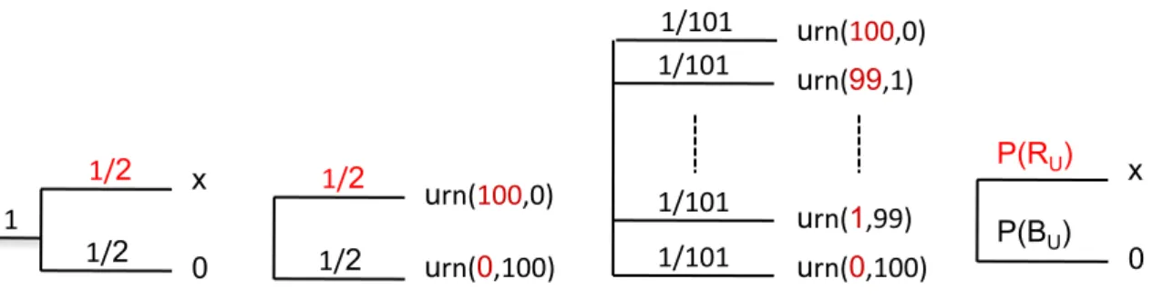
1.5.1 Two-urn experiment
Imagine two urns; the known urn contains fifty red balls and fifty black balls; the unknown
urn contains 100 balls that can be red or black but the proportion is not specified. The state
space is S= {0, 1, . . . , 100}where s corresponds to the state in which exactly s balls are red.
The payments of the DM are described by the set of possible consequences X = {0, x}, with
x >0.
Let us formalize Ellsberg paradox in the Anscombe-Aumann framework. The bet on red
(black) in the unknown urn is modeled through the horse race lottery f (f0) : S → L as
fol-lows: f(s) = s 100δx+ 100−s 100 δ0 and f 0(s) = 100−s 100 δx+ s
100δ0with δx the degenerate lottery that gives payoff x with certainty. The bet on red (black) in the known urn is represented
through g ( g0): g(s) = 1 2δx+ 1 2δ0 and g 0(s) = 1 2δ0+ 1
2δx. Ellsberg shows that, while being indifferent between betting on red or black within each urn ( f ∼ f0 and g ∼ g0), DMs may
reasonably prefer a bet on red (resp. black) in the known urn rather than a bet on red (resp.
black) in the unknown one ( g f and g0 f0). This preference for known (risky) over
unknown (ambiguous) bets is referred to by Ellsberg as ambiguity aversion.
Suppose now that preferences are represented by a subjective probability P on S and a
utility function u and assume u(0) = 0 and u(x) = 1. Thus, f ∼ f0 means ∑s∈SP(s)
s 100 =
1.5. ELLSBERG PARADOX ∑s∈SP(s) 100−s 100 which is equivalent to ∑s∈SP(s) s 100 = 1
2 meaning f ∼ g. This contradicts g f .
Ellsberg preference cannot be represented with subjective additive probability. Thus, PS
and SEU are violated.
1.5.2 One-urn experiment
One urn contains 90 balls; 30 are known to be red and the remaining 60 are known to be black
or yellow but the information about the precise proportion is missing. Ellsberg shows that
a DM who prefers a bet that gives a positive amount of money on {red} to an identical bet
on {black} (i.e., who is ambiguity averse in the same way as in the two-urn experiment), will
however prefer a bet that wins on {black and yellow} to a bet that wins on {red and yellow}.
Indeed, adding a winning event yellow to the initial bets should not affect the ranking
be-tween them (by P2). Choices are again driven by ambiguity avoidance and violate SEU and PS.
Ellsberg’s examples show that SEU and Machina and Schmeidler’s PS are violated as soon
as DMs exhibit ambiguity attitudes. Ambiguity attitudes contradict the Bayesian approach
that makes no difference between probabilities that are based on objective information and
probabilities that are built on a default in information. As argued by Schmeidler (1989)
the main limitation of SEU is that "The probability attached to an uncertain event does not
reflect the heuristic amount of information that led to the assignement of that probability.”
The models presented in the next section provide extension of SEU in order to account for
1.6. THE MODELING OF AMBIGUITY
1.6
The modeling of ambiguity
Ellsberg experiments (1961) rule out the possibility of modeling behavior under uncertainty
through consistent probability measures. The aim of this section is to present the models that
have been constructed in response to the paradox raised by Ellsberg. Each category of models
proposes a different way to solve the Ellsberg paradox. We distinguish four approaches in
the modeling of ambiguity.
The rank dependent approach, including Schmeidler (1989) and cumulative prospect
the-ory (Tversky and Kahneman, 1992), abandons subjective probabilities, allowing the
proba-bilities of events to be non-necessarily additive. The multiple prior approach preserves the
expected utility form but describes ambiguity through by means of a set of priors. The
multi-stage approach represents ambiguity as compound risk where the different stages of
the compound lottery are not necessarily reduced. The source of uncertainty approach
en-visages that each uncertainty subjectively covers different features and consequently, that all
uncertainties cannot be treated similarly in the decision process.
1.6.1 Choquet expected utility
The point of departure of the modeling of non additive probability is illustrated by the
fol-lowing example provided by Schmeidler (1989). Imagine a DM can bet on two coins. The
first coin has been extensively tested and was found to be fair. No information exists
re-garding the second coin. While the first coin carries enough evidence to be assigned with
a fifty-fifty distribution, the second will be naturally assigned the same distribution but by
invoking some other rule, typically Laplace’s principle of insufficient reason. The two
distri-butions, while being the same, feel different. Actually, the DM tends to consider that the two
bets are not equivalent, and he would be willing to bet less on the second coin (Gilboa et al.,
1.6. THE MODELING OF AMBIGUITY
probabilities that result from the absence of information.
Schmeidler (1989) finds the conditions to extend SEU to non additive probabilities. He
keeps Anscombe-Aumann’s A1, A3 and A4 and introduces the comonotonic independence
axiom and a monotonicity axiom.
Definition 5(Comonotonicity). Two acts f and g∈ F are comonotonic if there are no states s and s0 such that f(s) f(s0)and g(s0) g(s).
The following comonotonic independence condition replaces Anscombe-Aumann s’ A2.
A’2 (Comonotonic Independence)For all f , g, h∈ F, if f g, f and g are comonotononic with h, then λ f + (1−λ)h λg+ (1−λ)h
A’ 5 (Monotonicity)for all f , g∈ F, if f(s) %g(s)for all s∈S, then f % g
We need to introduce the definition of a non additive probability measure (also called
capacity):
Definition 6(Capacity). The function ν : S→ [0, 1]is a capacity if (i) ν(∅) =0, ν(S) =1 and (ii) E⊆F⇒ν(E) ≤ν(F).
In the following representation, outcomes of act f = [x1on E1; . . . ; xnon En]expressed in
monetary amounts are rank-ordered from worst to best x1 ≤ · · · ≤xn. Note that the ranking
of outcomes imply that the partition{E1; . . . ; En}of S is also rank-ordered.
Theorem 3(Schmeidler, 1989). Preferences satisfying axioms A1, A’2, A3, A4, A’5 have the follow-ing Choquet Expected Utility (CEU) representation:
CEU(f) =
n
∑
j=1
π(j)u(xj) (1.3)
where the decision weight π(j)is equal to ν(∪ni=jEj) −ν(∪ni=j+1Ej). Moreover, the capacity ν(.)on S
1.6. THE MODELING OF AMBIGUITY
The difference between CEU and SEU consists in the weights that precede utility when
evaluating an act. The weights P(Ej) under SEU are generated by an additive probability
measure on S while the weights π(j) under CEU are generated by a possible nonadditive
measure. The decision weight π(j) of event Ej depends on the event Ej and its ranking
position. Note that when ν(.) is additive, ν(∪ni=jEj) −ν(∪ni=j+1Ej) reduces to ν(Ej)and SEU
is obtained.
1.6.2 Multiple Prior models
The multiple prior approach assumes that the DM may not hold a unique belief on the states
of the world. Consequently, ambiguity is reflected by the multiplicity of priors. The extensions
of the original Maximin Expected utility (Gilboa and Schmeidler, 1989) consist in:
1. enlarging the attitudes towards ambiguity by allowing a continuum from extreme
pes-simism to extreme optimism in (i) combining the two extreme behaviors (min and max)
or (ii) adding an extraneaous ambiguity index.
2. taking into account the prior information available to the DM.
A similar but not equivalent approach consists in considering probability intervals for
events. Eventually, multiple priors can be related to possible incomplete preferences.
Maxmin expected utility
Gilboa & Schmeidler (1989) establish the axiomatization of Wald’s (1950) idea of maxmin
expected utility (MEU). The idea is as follows: when no information is available, it may be
too difficult for the DM to formulate a unique prior. In a way, it is less demanding to allow
the DM to consider a set of priors. This set is subjectively defined. For instance, an extreme
case would be to envisage all the possible probability distributions: in Ellsberg’s two-urn
1.6. THE MODELING OF AMBIGUITY
The axiomatic keeps Anscombe-Aumann’s A1, A3 and A4, adds A’5, replaces the
inde-pendence axiom (A2) by the certainty indeinde-pendence axiom (A"2) and adds an uncertainty
aversion axiom (A6).
FC is the set of constant acts, i.e, acts that give the same lottery whatever the state is;
elements of FC are indexed by c. A"2 is weaker than A2 since it requires that independence
holds whenever acts are mixed with a constant act hc.
A" 2 (Certainty-independence)for all f , g∈ F and hc ∈ FC, and for all λ∈]0, 1],
f g⇔λ f + (1−λ)hc λg+ (1−λ)hc
This following axiom captures the hedging phenomena. The DM should prefer a mixture
of two indifferent acts to each of these two acts.
A 6 (Uncertainty Aversion) for all f , g∈ F and λ∈]0, 1[, f ∼ g⇒λ f + (1−λ)g% f
The mixture operation reduces the uncertainty separately born by each act. We observe
that this axiom ex ante imposes a constraint on the DM’s reaction to ambiguity and thus MEU
will be able to describe Ellsberg type behavior.
It is worth remarking that adding this axiom to the CEU theorem results in a nonadditive
probability ν that satisfies convexity, i.e., ν(E) +ν(F) ≤ ν(E∪F) +ν(E∩F). Conversely, if ν
is convex, then the CEU preference relation satisfies A6.
Theorem 4 (Gilboa and Schmeidler, 1989). Preferences satisfying axioms A1, A"2, A3, A4, A’5 and A6 have a the following MEU representation:
MEU(f) =min
P∈C s
∑
∈SP(s)u(f(s)) (1.4) with u the utility function which is unique up to a positive linear transformation, and C the unique(closed and convex) set of priors P. Uniqueness ofC is given by A4.
1.6. THE MODELING OF AMBIGUITY
act for each prior probability distribution and then chooses the act that yields the highest
evaluation with respect to the worst prior distribution. We have seen that one prior
distribu-tion (the singleton set C = {P}, which corresponds to SEU) is not able to explain Ellsberg
preferences. However, we can see that a set of priors explains Ellsberg preferences. Take
the case where the set of priors C corresponds to L. With the usual normalization
condi-tions for utility (u(0) = 0 and u(x) = 1), Ellsberg preferences f ∼ f0 and g ∼ g0 imply
MEU(f) = MEU(f0) =0 and MEU(g) = MEU(g0) = 1
2 and these equalities are completely consistent with g f and g0 f0. It is worth noticing that the same result would be obtained
with a smaller set of priors (for instance, ifC = {priors such that s∈48, 49, 50}).
Maxmin is often viewed as associating the modeling of ambiguity to pessimism because of
the presence of the axiom of uncertainty aversion. However, nothing is said about the nature
of the set of beliefs that are revealed by the representation theorem. For instance, this set
may be assumed to comprise only optimistic probability distributions so that a DM who acts
pessimistically relative to his optimistic beliefs may finally behave in a less pessimistic way
than a true pessimist would have behaved. In short, behavioral traits that are not necessarily
due to ambiguity can be contained in the setC.
Moreover, it seems natural to interpret the size of C as a representation of the ambiguity
that the DM may perceive in the decision problem, but one problem with such interpretation
is the fact that the set C appears in Gilboa and Schmeidler’s analysis only as a result of
the assumption of ambiguity hedging. It therefore seems that the DM’s revealed ambiguity
cannot be disentangled from his behavioral response to such ambiguity. That is precisely
1.6. THE MODELING OF AMBIGUITY
α-MEU
Ghirardato, Maccheroni and Marinacci (2004) provide the axiomatization of the Hurwitz
cri-terion and extend MEU to allow for a more varied descriptions of ambiguity attitudes. α-MEU
combines both the maxmin and its extreme opposite maxmax (where the best probability is
considered) approaches. This combination permits us to account for all ambiguity attitudes
between maxmin and maxmax.
They distinguish between (i) the ambiguity perceived by the DM, which is given by a
set of probabilities C and (ii) the reaction of the DM to it, his ambiguity attitude, which is
captured by a unique coefficient α.
They first derive an "unambiguous preference” relation denoted by %∗ from the
prefer-ences of the DM that is built on a unanimity criterion: a DM unambiguously prefers (%∗) an
act f to an act g if the expected utility of act f is higher than the expected utility of g with
re-spect to every probability measure in the setC. The setCdescribes the DM’s revealed perception
of ambiguity1. A DM 1 perceives more ambiguity than a DM 2 if for all f , g f %∗
1 g⇒ f %∗2 g.
WhenC = {P}then%∗ is complete and corresponds to%. Hence, the DM 2 has a richer
un-ambiguous preference because she behaves as if she is better informed. Moreover, the size of
the set of priors gives information on the ambiguity attitude of a DM. Thus, in the previous
case, the DM 1 is more ambiguity averse than the second because she considers that more
probability distribution can occur (C1 is larger thanC2).
In a second step, ambiguity attitudes are represented through a parameter that captures
ambiguity attitudes. The following axiom guarantees that the certainty equivalent of f with
respect to%∗ (noted E∗(f)) contains all the information the DM uses in evaluating f .
A 7 For every f, g∈ L, E∗(f) =E∗(g) ⇒ f ∼ g
Theorem 5 (Ghirardato, Maccheroni, Marinacci, 2004). Preferences satisfying axioms A1, A"2,
1.6. THE MODELING OF AMBIGUITY
A3, A4, A’5 and A7 have the following α-MEU representation:
α−MEU(f) =αmin
P∈C
∑
S u(f(s))dP(s) + (1−α)maxP∈C∑
S u(f(s))dP(s) (1.5) Moreover,Cis unique, u(.) is unique up to an affine transformation and α∈ [0, 1]is unique ifCis nota singleton.
The DM’s reaction to ambiguity is captured by the ambiguity aversion coefficient α. The
set C is shown to be equal to the set of priors that Gilboa and Schmeidler derived in their
representation for α equal to 1. If α is equal to 0, maxmax is obtained. The set C yields
the smallest set of possible probability distributions that can be obtained, i.e, the closest
approximation of SEU.
Let us show that an ambiguity averse DM in the Ellsberg 90-ball urn experiment has an α
superior to 1/2. Let i defines the number of yellow balls and 60−i the number of black balls
in the urn. imin (resp. imax) is the minimum (resp. maximum) of i with respect to the set of
beliefs. A DM who prefers a bet on red (R) to a bet on yellow (Y) or similary black (B) reveals
(with the normalization conditions u(x) =1 and u(0) =0):
R Y⇒ 30 90 > αimin 90 + (1−α)imax 90
since the worth distribution is iminand
R B⇒ 30 90 > α(60−imax) 90 + (1−α)(60−imin) 90
since the worth distribution is imax.
By definition imax≥imin. Ellsberg type preferences R Y and R B imply that imin=imax
1.6. THE MODELING OF AMBIGUITY
Variational preferences
The variational preferences model (Maccheroni, Marinacci and Rustichini, 2006) is an
alterna-tive generalization of the multiple prior model.
The axiomatization conserves all MEU’s axioms except that the certainty independence
(A"2) is replaced by the weak certainty independence axiom (A2"’).
A 2”’ (Weak Certainty independence) if f , g∈ F and hc, h0c ∈ Fc, and λ ∈]0, 1[then, λ f + (1−λ)hc%λg+ (1−λ)hc⇒λ f + (1−λ)h0c%λg+ (1−λ)h0c
The certainty independence axiom actually involves two types of independence:
indepen-dence relative to mixing with constant acts and indepenindepen-dence relative to the weights used in
such mixing. A"’2 retains the first form of independence, but not the second one. They
al-low for preference reversals in mixing with constants unless the weights themselves are kept
constant.
Theorem 6(Maccheroni, Marinacci and Rustichini, 2006). Preferences satisfying axioms A1, A”’2, A3, A4, A’5, A6 are variational and have the following representation:
VP(f) =min
P∈D
Z
Su
(f(s))dP(s) +b(P) (1.6)
where b is an ambiguity aversion index from D(Σ)to(0,+∞)where D(Σ)is the set of all probability distributions onΣ, an algebra over S.
Variational preferences are ambiguity averse due to A6. The lower is b, the higher is the
ambiguity aversion exhibited by the DM. b associates a weight to each probability distribution
P. A relation%1 more ambiguity averse than%2 is equivalent to (u1 =u2 and b1 ≤b2). MEU
with the set of priorsC is a special case of the variational preferences where b(P) =0 if P∈ C
1.6. THE MODELING OF AMBIGUITY
Ambiguity as imprecise information
In the previous models, nothing is said about the informational structure of the decision
prob-lem and the models themselves do not envisage the case where the DM possesses objective
information in the sense where it does not explicitly appear in their construction.
Informa-tional aspects, if they exist, appear in the revealed set of beliefs as an output of the decision
process. However, in most decision situations data is often available to the DM even vague or
imprecise.
For instance, in Ellsberg’s three-color problem, the prior information is the set of
proba-bility distributions that admit the probaproba-bility 1/3 on the event ’drawing a red ball’. Thus, the
DM has information since the probability interval for drawing a black or yellow ball is smaller
than the unit interval that would correspond to full ambiguity. Gajdos, Hayashi, Tallon and
Vergnaud (2008) specifically aim at modeling information as a part of ambiguity.
They describe the informational structure of a decision context by P that represents the
objective a priori information and r a reference prior also called anchor (r belongs to the
convex hull of P). For instance, in the three-color problem, the set of priors appropriate to
model available information is the set of all probability distributions that place 1/3 on red.
The reference prior of this set is the natural distribution(1/3, 1/3, 1/3)(by symmetry).
The concept of reference prior is central in this model since aversion towards imprecision
is built around it. Indeed, one situation is considered more imprecise than another if the set
of probability distributions considered possible in the second situation is included in the set
of the first. In Ellsberg’s two-color example, having one red and nighty-nine black is more
precise that no information about the proportion of the two colors, but it seems reasonable to
assume that a DM would prefer to bet on red in the ambiguous urn than in the more precise
known urn. Thus, a proper description of information requires a condition on anchor.
1.6. THE MODELING OF AMBIGUITY
is more imprecise than P2 and (ii) r1 = r2 (they have the same center). For instance, in the
two-color problem, if there are two balls in the ambiguous urn, the information is described
by P1 = {(1, 0),(0, 1)} and the center is(1/2, 1/2); if there are three balls in the ambiguous
urn, the information P2 = {(1, 0),(2/3, 1/3),(1/3, 2/3),(0, 1)}has the same center (1/2, 1/2).
Hence, the imprecision of the two situations is the same (the number of balls considered as
immaterial).
In this model, the DM ’s preferences are defined on both act and information. The
repre-sentation theorem allows two acts to be compared in two different informational situations.
(f ,[P1, r1]) % (g,[P2, r2]) ⇔ α min p∈co(P1) Z Su (f(s))dp1(s) + (1−α) Z Su (f(s))dr1 ≥ α min p∈co(P2) Z Su (g(s))dp2(s) + (1−α) Z Su (g(s))dr2 (1.7)
The functionnal form is a convex combination of the minimum expected utility with respect to
probability distributions in the set of objectively admissible probability distribution and of the
expected utility with respect to the anchor. The revealed set is a subset of the set of admissible
probability distributions. Hence, an extremely pessimistic DM will keep the entire initial set
of admissible priors. Conversely, a DM not affected by imprecision reduces any prior set of
probability distribution to the anchor distribution. α measures the degree of pessimism. If α
is equal to zero, the DM is EU with respect to the anchor, and if α is equal to one, he is MEU
with respect to all distributions compatible with information.
Ambiguity and indecision
For many authors, (Mandler 2005, among others), the completeness assumption - which