Longevity and Economic Growth : three Essays

de

PSL Research University

Préparée à

-Dauphine

Soutenue le

par

cole Doctorale de Dauphine

ED 543

Spécialité

Dirigée par

Longevity and Economic Growth: Three Essays.

08.11.2016

Paris School of Economics

Aix-Marseille Université University of Oregon Université Paris-Dauphine Université Paris-Est

Sciences économiques

1

L’Université Paris-Dauphine n’entend donner aucune approbation ni improbation aux opinions émises dans les thèses ; ces opinions doivent être considérées comme propres à leurs auteurs.

3

Qui veut s’élever au-dessus des hommes doit se préparer à une lutte, ne reculer devant aucune difficulté. Un grand écrivain est un martyr qui ne mourra pas, voilà tout.

Honoré de Balzac, Illusions Perdues

5

Remerciements

Je remercie en premier lieu Najat El Mekkaoui de Freitas d’avoir accepté d’encadrer ce travail doctoral. Je lui suis reconnaissant pour ses nombreuses suggestions, relectures et critiques de mon travail qui m’ont permis de l’améliorer tout au long de cette thèse. Je la remercie également pour son aide dans ma recherche d’un contrat postdoctoral et pour m’avoir présenté à de nombreux chercheurs. Enfin, je la remercie pour sa composition de mon jury de thèse. Je suis honoré par la participation de chacun de ses membres.

Je remercie Hippolyte d’Albis et Gregory Ponthiere d’avoir accepté d’être mes rappor-teurs. Je les remercie pour leurs nombreuses remarques et suggestions durant ma présoute-nance. Je remercie aussi Hippolyte d’Albis pour ses commentaires sur des versions prélimi-naires des chapitres 1 et 3.

Je remercie Raouf Boucekkine d’avoir accepté d’être membre de mon jury. Je le remer-cie également de m’avoir accueilli à Marseille pour discuter d’une version préliminaire du chapitre 1.

I thank Shankha Chakraborty for accepting to be member of my PhD committee. It is a great honour for me to discuss my work with him.

Je remercie Philippe de Vreyer d’avoir accepté d’être membre de mon jury. Je le remercie également de m’avoir accueilli au sein du laboratoire DIAL, de m’avoir confié des groupes de travaux dirigés ainsi que d’avoir toujours répondu positivement à mes demandes de finance-ment pour des conférences.

Je remercie Vincent Iehlé, Bernard Masson et David Ettinger pour m’avoir confié des groupes de travaux dirigés. Je remercie aussi Vincent Iehlé pour ses commentaires sur le chapitre 1, pour sa disponibilité ainsi que pour son soutien dans ma recherche d’un contrat postdoctoral.

I have benefited from discussions with Marcello d’Amato and Paul Romer, whom I would like to thank both.

Je remercie les camarades et amis dauphinois qui m’ont accompagné durant ces quatre années : Anne-Charlotte, Ano, Daniel, Florence, José, Julien, Léo et Nicolas. Je remercie Benoît pour sa relecture minutieuse du manuscrit.

Je remercie ma famille : mes parents, mes deux soeurs, Alice et Caroline, et mon oncle. Cette thèse leur est dédiée.

Contents 6

List of Figures 8

List of Tables 9

Introduction 11

1 Endogenous lifetime and economic growth : the role of the tax

rate 17

1.1 Introduction . . . 17

1.2 The model . . . 20

1.3 The influence of the tax rate on the growth rate and on the SS income level . . . 22

1.3.1 The growth-maximizing tax rate . . . 22

1.3.2 The impact of the tax rate on the SS income level . . . 24

1.4 Impact of the tax rate on the SS welfare . . . 25

1.4.1 u(c) =ln(c)case : . . . 26 1.4.2 u(c) = c1−σ 1−σ case :. . . 27 1.5 Conclusion . . . 28 1.6 Appendix A . . . 29 1.7 Appendix B . . . 30 1.8 Appendix C . . . 32 1.9 Appendix D . . . 34 1.10 Appendix E . . . 37

2 Growth, longevity and endogenous health expenditures 41 2.1 Introduction . . . 41

2.2 The model . . . 44

2.2.1 Outline . . . 44

2.2.2 Firms. . . 44

2.2.3 Preferences . . . 45

2.2.4 Partial equilibrium results . . . 45

2.3 The dynamic general equilibrium . . . 49

2.3.1 Dynamics in the case p=0. . . 50

2.3.2 Dynamics in the case p>0. . . 50

2.4 Discussion and numerical illustration . . . 54

2.4.1 Alternative preferences . . . 54 2.4.2 Numerical application . . . 55 2.5 Conclusion . . . 58 2.6 Appendix A . . . 59 2.7 Appendix B . . . 60 2.8 Appendix C . . . 61 2.9 Appendix D . . . 63 2.10 Appendix E . . . 65 2.11 Appendix F . . . 65 2.12 Appendix G . . . 65

3 Aging and sectorial labor allocation 69 3.1 Introduction . . . 69

3.2 Longevity in a multi-sector Diamond economy : partial equili-brium analysis . . . 72

3.2.1 Outline of the model . . . 72

3.2.2 Intratemporal reallocation of resources at the individual level . . . 72

3.2.3 The allocation and the population effect . . . 74

3.3 General equilibrium . . . 79 3.3.1 Firms. . . 80 3.3.2 Preferences . . . 80 3.3.3 Equilibrium . . . 82 3.3.4 Numerical analysis . . . 90 3.4 Conclusion . . . 95 3.5 Appendix A . . . 96 3.6 Appendix B . . . 97 3.7 Appendix C . . . 101 3.8 Appendix D . . . 102 3.9 Appendix E . . . 104 3.10 Appendix F . . . 105 3.11 Appendix G . . . 107 3.12 Appendix H . . . 107 3.13 Appendix I . . . 108 3.14 Appendix J . . . 109 Conclusion 111 References 113 7

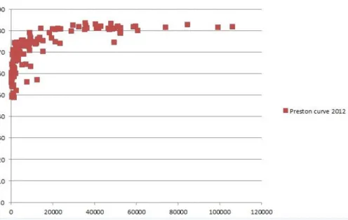
1 GDP per capita (x-axis) and life expectancy (y-axis) across countries (2012).

Source : World Bank database. . . 14

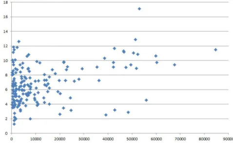
1.1 GDP per capita and ratio of total health expenditures to GDP across countries (2012). Source : World Bank database. . . 18

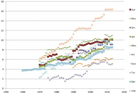
2.1 Ratio of total health expenditures to GDP in 10 OECD countries . . . 42

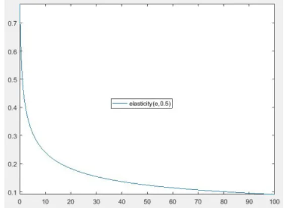
2.2 Health elasticity to consumption elasticity ratio (i.e. e_→ p_p′(₍e_e)₎e(1−σ)). p(e) = e0.5 1+e0.5, σ=0.5. . . 49

2.3 Income share spent on health as a function of income (i.e. w_→ x(w)). p(e) = e0.5 1+e0.5, σ=0.5, R=4.801. . . 49

2.4 Health expenditures-Life expectancy . . . 57

2.5 Income-Income share spent on health . . . 57

2.6 Wage dynamics over 10 periods . . . 57

2.7 Income share spent on health dynamics over 10 periods . . . 57

3.1 Y, O and Y+O. . . 78

3.2 Change of C1t C2t after a longevity shift with homothetic and non-identical prefe-rences. . . 78

3.3 Change of C1t C2t after a longevity shift with non-homothetic preferences. . . 78

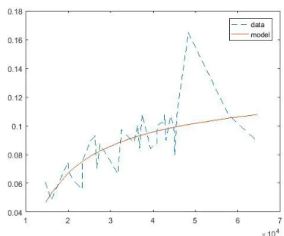
3.4 q_→ l1t l2t for n=1.52, t=2010 . . . 92

3.5 n_→ l1t l2t for q=0.4, t=2010 . . . 92

3.6 Time evolution of l1t l2t for different demographic parameters . . . 93

3.7 q_→ lIt l1t+l2t for n=1.52 . . . 93 3.8 n_→ lIt l1t+l2t for q=0.4 . . . 93 3.9 q_→yt for n=1.52 . . . 94 3.10 n_→ytfor q=0.4 . . . 94 8

LIST OF TABLES 9

List of Tables

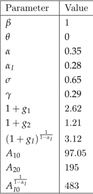
3.1 Parameter values used in the numerical analysis . . . 92 3.2 Percentage change of l1t

l2t,

lIt

l1t+l2t , ytwhen(q, n)changes from(0.4, 0.52). . . 94

3.3 Percentage change of l1t

l2t and

lIt

Introduction

Current income per capita in the US is about 15 fold that of Sub-Saharan countries. Un-derstanding income disparities across countries has been one of the main question addressed by economists since The Wealth of Nations by Adam Smith (1776). The possibility for longe-vity to be one important factor shaping these disparities has only started to be considered in the last fifteen years. This contrasts with another demographic variable, fertility, which has played a central role in the theory of economic growth since the essays of Malthus (1807). Indeed, for most of human history, countries have been trapped in the Malthusian regime, in which the level of technological advancement is not correlated with the income level, yet with the population density : further technological progress allows individuals to have more children, which annihilates income per capita gains. The break-up of this mechanism is a necessary condition for countries to enter the modern growth regime. Weil and Galor (1999) argue that this is made possible by a change in the nature of technological progress that becomes more and more skill-demanding. This creates an incentive for individuals to have fewer children and to invest more in their education, which marks the onset of standards of living improvements.

More recent contributions underline the role of life expectancy improvement in this change of regime and as an important dimension to take into account in the economic growth theory. Boucekkine et al. (2004) advance that the exit of the Malthusian regime is not a consequence of a greater demand for human capital, as suggested by Weil and Galor (1999), but is due to a greater human capital supply caused by more favourable climatic conditions that improve life expectancy. At the heart of their explanation is the so-called Ben-Porath mechanism : as longevity increases, the time period during which individuals can benefit from their schooling investments increases, which stimulates human capital supply. To gain intuition, consider the case of individuals facing low survival chances. Oster et al. (2013) study the college attendance decision of a sample of individuals who have a parent with Huntington disease. This illness, which has a one-half probability to be transmitted to child, limits the life expectancy of an infected individual to 20 years after symptoms begin. Oster et al. (2013) show that individuals discovering their genetic mutation during high school are 30% less likely to attend college than those who do not. Furthermore, the earlier the symptoms begin, the earlier individuals stop their schooling as the Ben-Porath mechanism suggests. Note that this effect directly arises from the lifetime budget constraint of individuals : with an increasing utility function, that does not depend on schooling, the best schooling time is the one that maximizes lifetime income and it is increasing with the number of years the

dual can work. However, for agents that make their decisions by maximizing their lifetime utility function, longevity also directly enters their preferences. To see how this interacts with their decisions, consider again the case of individuals facing a limited life expectancy. Lorentzen et al. (2008) study their behavior on a sample composed of people living near the power plant of Tchernobyl during the catastrophe and individuals infected by HIV. They show that these individuals engage into more risky behaviors such as : smoking, drinking, unsafe sexual relationships. Indeed, these individuals know that they cannot enjoy utility in the future, so they dedicate all their resources, here particularly their health capital, to maximize their present utility which merges into their lifetime utility. However, this is unlikely to compensate the welfare loss due to their premature death because they still have a decreasing marginal utility. On the contrary, individuals who do not face low survival chances can get a greater lifetime welfare by choosing to channel resources in the future. Furthermore, individuals can decide to spend resources to increase their future survival chances to enjoy consumption utility for a longer period. In other words, physical capital supply is also driven by health conditions. This is a second link, first highlighted by Bloom et al. (2003) and Chakraborty (2004), through which longevity and economic growth interact. As human and physical capital are the main production factors, this helps to understand the results of Weil (2007) according to whom up to 20% of across countries income per capita dispersion can be explained by differences of adult survival rates. Thus, studying the role played by health in economics contributes to better understand the mechanics of economic development. This PhD dissertation proposes three essays on the links between health and economic development. More specifically, I will address the three following questions : (i) Can a country experience a higher economic growth rate by spending more on health ? (ii) Do health expenditures endanger economic growth ? (iii) How does the aging process affect the income level and the sectorial labor allocation of a multi-sector economy ?

In addition to the theoretical insights quoted previously, a link between life expectancy and income per capita can be sensed from the observation of the trajectories of the two variables. For most countries, they both fluctuate around a nearly constant value during most of human history before entering a positive growth regime at different dates. More precisely, consider the case of England, the first country to enter the modern growth regime. Evolution of life expectancy has paralleled that of income with some lags. Life expectancy was 39,24 in England in 1820. It was still close to this value in 1850 (40,6), while during the same period income per capita has increased by 41%.1 Then, except during war periods, both life expectancy and income have been increasing.2_{Life expectancy is now more than the}

double of its value in 1820, while income has been multiplied by more than 13. The picture

1. Historical data on life expectancy are from de la Croix and Sommacal (2009), while those on income are from Fouquet and Broadberry (2015). Any other data used in the introduction, whose source is not mentioned, are obtained from the World bank database. Income is GDP per capita in current US dollars.

2. There are exceptions to this in developed countries. In Russia, life expectancy has decreased after the fall of the soviet union. Case and Deaton (2015) document a rising mortality in midlife among white non-Hispanic Americans during the period 1999-2014.

Introduction 13

of developing countries is more contrasted. Overall, thanks to the eradication of smallpox, which was responsible for 2 million deaths a year until the end of 1960, health conditions have improved (Bloom et al. 2005).3This is confirmed by the world life expectancy evolution which increased from 52 in 1960 to 71 in 2013. In East Asia, life expectancy stands at 76, while it was 46,4 just after WWII. In Sub-Saharan countries, average life expectancy has increased from 51 to 58,1 over the last decade. However, in terms of income evolution, large disparities exist. In 1962, income per capita of East Asia was 4.3% that of the US, while income per capita of Subsaharan Africa was 4.1% that of the US. In 2014, income per capita of East Asia was 18% that of the US, while income per capita of Subsaharan Africa was 3% that of the US. Regarding Sub-saharan Africa, current life expectancy in the region corresponds to the one of England in 1925. Yet, income per capita at that time exceeded by more than 60% the current level in Sub-saharan countries.

These empirical facts are well captured by the Preston curve (see Figure 1). Preston (1975) estimates the cross-sectional relationship between income per capita and life expectancy. He observes a concave and increasing relationship between the two variables. The concavity of the curve is a consequence of the quasi complete convergence of some developing countries in terms of life expectancy while their convergence in terms of income is still incomplete. For example, life expectancies of US and China, respectively equal to 79 and 75, only differ by 5%, while the income per capita in US is more than sixfold the one of China. The fact that current Sub-saharan individuals live as long as European did in 1925, while their income is only 60% of the English level in 1925 is an illustration of the upward shift with time of the curve.

Understanding the origin of the Preston curve is a mirror problem of understanding the link between life expectancy and income. The curve reflects the causal impact of life expec-tancy on income, the reverse causality as well as the influence of other correlates. Dalgaard and Strulik (2014) argue that about 80% of the Preston curve can be attributed to the causal effect of income on life expectancy : richer countries can spend more resources on health, for example, by implementing better medical facilities and public infrastructure such as raw sewage disposals that reduce the propagation of diseases. A contrario, empirical evidence on the causal impact of life expectancy on income are contrasted, leaving 20% of the relationship between income and life expectancy unexplained. Acemoglu and Johnson (2007) and Ashraf et al. (2008) find no significant effect of life expectancy on the growth rate of income per capita, while Aghion et al. (2011) and Sunde and Strittmatter (2013) find a positive effect of life expectancy on economic growth. These results are unexpected from two perspectives. First, microeconometric studies unambiguously claim that healthier individuals get a higher income.4 Second, it is unexpected from life cycle theory, as I mentioned it previously, these

3. As for developed countries, some countries have undergone a decrease of life expectancy particularly be-cause of HIV epidemics. This is the case for South-Africa and Namibia. In South-Africa, life expectancy was 62 in 1992, while it was 52 in 2005. In Namibia, life expectancy was 61 in 1991, while it was 54 in 2003.

Figure1 – GDP per capita (x-axis) and life expectancy (y-axis) across countries (2012).

Source : World Bank database.

models predict that a greater longevity should stimulate both human and physical capital supply. As pointed out by Acemoglu (2010), this means that there are general equilibrium effects at stake.5 Thus, in this PhD dissertation, I will study theoretically how life expec-tancy interferes with income from dynamic general equiilibrium models. Not only does the understanding of the causal impact of life expectancy on income enables to understand how previous health improvements have contributed to shape the wealth of Nations, but it also enables to better understand how income will evolve in the future as life expectancy will pursue its upward trend. Indeed, evolution of life expectancy in developed countries, coupled with that of fertility, is such that they enter the aging phase : the ratio of workers to people aged more than 65 is increasing. Indeed, the dependency ratio, the ratio of people aged less than 20 or more than 65 to those aged between 20 and 65, currently at 68,35% in OECD countries, is expected to reach 86,7% in 2050 according to OECD.

In various dynamic general equilibrium settings, I will study the consequences on the econo-mic outcome of an exogenous shock on the longevity parameter or I will study the possibility for the longevity to be itself an endogenous variable. There are two types of economic models that I will use extensively for the analysis. The first step, at the microeconomic level, is to de-rive the behavior of agents, particularly with respect to their longevity, through the life cycle hypothesis. Pioneered by Modigliani and Brumberg (1954), this theory hypothesizes that in-dividuals allocate their lifetime resources in order to maximize their lifetime utility function. Thus, longevity naturally enters the individual decisions as opposed to the infinite horizon framework used in standard growth models. The second step consists in the aggregation of

5. d’Albis et al. (2012) and Sunde and Cervellati (2013) suggest that a life expectancy increase can be the result of an increase of survival probabilities at different ages, which can activate life-cycle mechanisms differently. For example, schooling time responds to increases in survival probabilities in adulthood and not to survival probabilites in retirement period.

Introduction 15

the behavior of agents differing with respect to their birth dates to determine the equilibrium of the economy. This is precisely what overlapping generations (henceforth OLG) models allow to do. Pioneered by Allais (1947), Samuelson (1958) and Diamond (1965), OLG models are microfunded macroeconomic models in which agents may differ with respect to their age. They represent a natural tool to introduce demographic variables into macroeconomic studies. Blanchard (1985) is the first who explicitly introduced longevity as an exogenous variable in an OLG model using a version of the life-cycle model of Yaari (1965). There are numerous declinations of this type of work in growth models with different growth engines. For instance, Boucekkine et al. (2003) translate a life-cycle model à la Ben-Porath (1967) into an OLG model, while Prettner (2013) examines the consequences of a longevity shift in an endogenous growth framework. Chapter 3 places itself in this kind of analysis, that I extend to multi-sector growth models. Indeed, in a multi-sector Diamond model, I study how the labor allocation of the economy is impacted by a longevity shock and I show that these labor reallocations can produce negative effects on the income per worker level. The second type of studies of longevity in OLG economies is due to Cipriani and Blackburn (2002) and Chakraborty (2004). They formulate OLG models in which the longevity is no more a parameter, but an endogenous variable. In Cipriani and Blackburn (2002), human capital investments exert a positive externality on longevity, while in Chakraborty (2004) there is a government that taxes at a constant rate the wage of individuals to finance public health expenditures that increase longevity. In the first chapter, this paper is extensively quoted as I argue that the potential of his framework has not been fully exploited. Indeed, I will study how the tax rate influences the transitional dynamics as well as the steady state of the economy. In the second chapter, I will propose an OLG model with endogenous lifetime in which the agents choose their level of health expenditures. More specifically, the dissertation is organized into three chapters which can be summarized as follows.

In the first chapter, I study the impact of health expenditures on economic growth and on welfare. For this, I draw on the seminal contribution of Chakraborty (2004). In his two-period overlapping generations model with a lifetime depending on public health expenditures, I study the influence of the tax rate, which is an exogenous parameter in Chakraborty (2004), on the economy. First, I determine the growth-maximizing tax rate, which is shown to be 0 in low-income countries. Second, I show that the steady-state income level is an inverted U-shaped function or a decreasing function of the tax rate. Third, I study the tax rate that maximizes the steady-state welfare level.

In the second chapter, I propose a theoretical model to study the growth impacts of health expenditures chosen by the agents. Indeed, I develop a Diamond model with endogenous growth in which young individuals can spend resources to increase their longevity in retire-ment period. First, I derive the demand for health and show that the income share spent on health is an inverted U-shaped function of income. Second, I fully characterize the dynamic general equilibrium and determine the growth impacts of the health expenditures. Several cases can occur. Health expenditures can speed up or slow down economic growth. They can be a barrier to growth or they can be a necessity for growth to take place. A simple

calibration of the model to OECD countries suggests that the latter case is the most likely one.

Finally, the third chapter determines the theoretical impact of the aging process on the sectorial allocation of labor. To this aim, I build a multi-sector two-period overlapping gene-rations model in which I examine the consequences of both a longevity shift and a fertility shift on the labor allocation of the economy. There are three effects at stake : (i) Given prices, a longevity shift directly affects consumption levels of the individuals. (ii) Given the consumption levels of young and old individuals, aging increases the ratio of old to young individuals. (iii) Aging affects the price vector of an economy through its impact on the ac-cumulation of production factors. These effects change the relative demand between sectors, which modifies the labor allocation. I first state necessary and sufficient conditions for aging to create intratemporal reallocation of resources at the individual as well as at the aggregate level in partial equilibrium. Then, I study the dependence of the labor ratios between sectors with respect to demographic variables along a path satisfying the Kaldor facts.

1

Endogenous lifetime and

economic growth : the role of

the tax rate

1.1

Introduction

The last decade has been the stage of a vivid academic debate on the health-growth nexus. This was stimulated by reports from International Organizations advocating health enhan-cing policies (see Acemoglu and Johnson (2006)). According to their views, the benefits of these policies are two-fold : (i) Improving health has positive welfare impacts. (ii) Improving health spurs economic growth. For example, Weil (2014) quotes the following passage of the WHO commission report :

Improving the health and longevity of the poor is an end in itself, a funda-mental goal of economic development. But it is also a means to achieving the other development goals relating to poverty reduction. The linkages of health to poverty reduction and to long-term economic growth are powerful, much stronger than is generally understood. The burden of disease in some low-income regions, especially sub-Saharan Africa, stands as a stark barrier to economic growth and therefore must be addressed frontally and centrally in any comprehensive deve-lopment strategy.

Over the period 1950-1990, the life expectancy increase in developing countries is well-documented (Bourguignon and Morrison 2002 ; Becker et al. 2005). Even though HIV caused life expectancy reversals in some countries such as in South-Africa or Namibia, overall pro-gresses can be observed from the increase of the world life expectancy average from 52 in 1960 to 71 in 2013.1_{This is particularly due to reductions in infant mortality rates (Cutler et al.}

2006). Although survival rates of children in developing countries have not reached those of developed countries, future gains in life expectancy in developing countries will mainly pass through health improvements at older ages. While Acemoglu and Johnson (2006) attribute

1. These numbers and the others used in the introduction are all obtained from the World Bank database.

the past health improvements to the diffusion of new drugs and new medical practises, survi-val gains at older ages will depend on domestic health expenditures (Cutler et al. 2006). This motivates us to ask whether statements (i) and (ii) are valid when health improvements are costly.

In Figure 1.1, I plot the ratio of total health expenditures to GDP as a function of GDP per capita across countries. While the share of resources spent on health seems to increase with income when income is not too low, there is no clear relation between the two variables when income is low. Sierra Leone spends almost 12% of its income on health, which is almost the share spent by France, while the income per capita of France is 25 times that of Sierra Leone. On the contrary, in Lao or Pakistan, this ratio is less than 2.75%. This raises several questions : Can a low-income country spur economic growth by spending more resources on health ? From a welfare point of view, can it be optimal for a country not to spend resources on health ? This paper uses theory to answer these questions. Otherwise said, I determine analytically if statements (i) and (ii) remain valid when health improvements are not free of cost.

Figure1.1 – GDP per capita and ratio of total health expenditures to GDP across countries (2012).

Source : World Bank database.

More precisely, I extend the results of Chakraborty (2004), who builds a Diamond model with a survival probability into second period that depends on public health expenditures. Indeed, I study the impact of the tax rate, which is an exogenous parameter in Chakraborty (2004), on the income level and on the welfare in the steady state (hereafter SS) to answer the two following questions : How does the income level vary with respect to the tax rate ? Is the welfare-maximizing tax rate always positive ? Doing this, I complement a large theoretical literature on the health-growth nexus that has got interested into statements (i) and (ii).

Statement (ii) has received much attention in the literature. On the empirical side, the re-sults are contrasted. Aghion et al.(2011) observe a positive impact of life expectancy growth rate on GDP per capita growth rate. Instrumenting life expectancy by the introduction date

1.1. Introduction 19

of a public health care system, Strittmatter and Sunde (2013) also find a positive effect of life expectancy on GDP per capita growth rate. On the other hand, Acemoglu and Johnson (2007) argue that the positive impact of health on GDP growth is counteracted by a popula-tion increase so that GDP per capita of health improvements become non-significant. Using a simulation approach, Ashraf et al.(2008) also conclude that the income benefits of health improvements are negligible. On the theoretical side, authors have examined the impact of the life expectancy parameter on the income level in various dynamic general equilibrium frameworks. In a R&D based-growth model, Prettner (2013) shows that a longevity increase has a positive effect on the income per capita growth rate. In a growth model with human capital investments, de la Croix and Licandro (1999) show that a longevity increase induces two counteracting effects on the growth rate. On the one hand, the Ben Porath effect in-creases human capital supply. On the other hand, this leaves more retirees and more people educated a long time ago. Finally, when capital accumulation is the growth engine, longevity increases are seen as positive because they increase the propensity to save of the individuals and then economic growth (Bloom et al. (2003) and Chakraborty (2004)). These results are causal statements that neglect the possible costs of longevity improvements.

My contribution to the literature that has studied statement (ii) is to determine the impact on economic growth of costly longevity improvements. Closely related to my work are Chakraborty (2004) and Bhattacharya and Qiao (2007). Both papers are based on Diamond model with an endogenous survival probability into second period. In Bhattacharya and Qiao (2007), the survival probability depends on both private health expenditures, whose level is chosen by the agent, and public health expenditures, whose financing tax rate is an exogenous parameter.2 _{The authors show that the SS income per worker level is an inverted U-shaped}

function of the tax rate. Here I aim to determine how the income per worker level depends on the total level of health expenditures. To do this, I abstract from the financing source of health expenditures and directly build on the model of Chakraborty (2004) by considering that all health expenditures are public. Then, I assess how the SS income level depends on these health expenditures. The question is not trivial because health expenditures create a trade-off on savings, hence on economic growth as capital accumulation is the growth engine in our specification. On the one hand, health expenditures increase longevity and so the propensity to save (Bloom et al. (2003) and Chakraborty (2004)). On the other hand, health expenditures reduce the disposable income and so savings. From this framework, I can also provide results on the welfare impact of health expenditures in SS, hence I can assess if the theory is also in line with statement (i).

Statement (i) has been much less examined by economists. Becker et al. (2005) argue that life expectancy improvements in developing countries in the XXth _{century significantly}

improved welfare. Murphy and Topel (2006) assess the social value of longevity gains in US on the previous century and show that it is potentially large. Theoretically, the literature has also discussed normative aspects of health expenditures particularly the decentralization

2. The authors also make a simplifying assumption, that I do not follow here, according to which only old agents derive utility from consumption.

of social optimum in the context of health related externalities.3 For example, Jouvet et al.(2010) and Ponthiere (2016) discuss the decentralization of social optimum in economies in which pollution exerts negative externalities on the longevity of individuals. To the best of my knowledge, the literature has not discussed whether positive health expenditures maxi-mize welfare in an environment free of externalities. However, there are reasons to believe that the level of health expenditures that maximizes welfare is not necessarily positive. Even though marginal utility of longevity is positive, longevity improvements can decrease welfare as they can diminish the level of resources per period. Second, health expenditures reduce the disposable income of individuals. Third, it is possible that health expenditures decrease the SS income level. This leaves three possible negative forces on welfare that health expen-ditures can exert. This justifies to investigate carefully whether the welfare-maximizing level of health expenditures is necessarily positive.

The rest of the paper proceeds as follows. Section 1.2 outlines the model of Chakraborty (2004) with two slight modifications. Section 1.3 studies the growth-maximizing tax rate and the tax rate that maximizes the steady-state income level. Section 1.4 studies the welfare-maximizing tax rate. Section 1.5 concludes.

1.2

The model

The model follows the one outlined by Chakraborty (2004). Consider a two-period OLG model in which the survival into second period occurs with probability pt for an individual

born at time t. pt is taken as exogenous by the individuals. The number of young agents is

constant and normalized to 1. Agents work during the first period and retire in second period. The consumption plan of a cohort-t individual is chosen by maximizing the following lifetime expected utility function :

Ut =u(c1t) +ptu(c2t+1) (1.1)

Subject to the budget constraints :

c1t+st≤ (1−τ)wt and c2t+1≤ 1+_pr_tt+1st.

Where c1t is the first period consumption, c2t+1 the second period consumption, rt+1the

interest rate. τ is the tax rate on wages imposed by the government. st are the savings that

are invested in capital by mutual funds. Assuming perfect competition among mutual funds, as in Yaari (1965), implies that the rate of return is 1+rt+1

pt

u is the utility per period function. I will consider two different specifications for u : u(c) =ln(c)(case (A)) and u(c) = ₁c1₋−_σσ, with σ<_{1 (case (B)). Case (A) is the one considered}

by Chakraborty (2004). In this case, utility becomes negative when the income level is low, which yields a negative marginal utility of longevity. As long as longevity is not chosen by the agent, this has no consequences, however in section 1.4 when I determine the welfare-maximizing tax rate, this property is crucial. To determine if my results are sensitive to the

1.2. The model 21

positiveness of the utility function, I also consider case (B), in which utility level is positive for any income levels. Hence, marginal utility of longevity is always positive. Case (B) is used in growth models in which health expenditures are chosen by individuals such as Chakraborty and Das (2005) and Bhattacharya and Qiao (2007).

It follows that savings are given by :

st= pt

(1+rt+1)

σ−1

σ +p_t

(1−τ)wt (1.2)

Where σ=1 is case (A), while σ <1 is case (B).

The final good is produced with labor, Lt, and capital, Kt. It is consumed or invested in

physical capital or used by the government to increase longevity. The production function is Cobb-Douglas : Yt = AKtαLt1−α with A>0 and α∈ (0, 1). Inputs are paid at their marginal

productivity. Using the fact that the workforce size is 1, I get that :

1+rt= AαKαt−1 (1.3)

and

wt = A(1−α)Ktα (1.4)

Where I have assumed that capital fully depreciates at each period. pt has yet to be

specified. The government finances public health expenditures with a balanced budget and pt is an increasing and strictly concave function of health expenditures per young person :

pt= p(τwt).

Where p satisfies :

p(0) = p>_{0, lim}

x→∞(p(x)) = p≤1, p

′_{(0) =γ}< ∞ (1.5)

I will also consider the limit cases p=0 and γ=∞ to see how they change my results.

τ is taken as constant in this section. I will study the influence of τ in the next two

sections. Finally, the dynamics of the economy is obtained by imposing the equilibrium on the capital market :

Kt+1 = p (τA(1−α)Kα_t) (Aα)σ−σ1K 1−σ σ (1−α) t+1 +p(τA(1−α)Kαt) (1−τ)A(1−α)Kαt (1.6)

The study and the interpretation of (1.6) in case (A) can be found in Chakraborty (2004). Here I add a sufficient condition for the SS of (1.6) to be unique. Moreover, I study the dynamics in case (B) and provide a sufficient condition for the SS uniqueness. Taking care of the uniqueness of the SS is necessary for the following sections in order to define economic variables in SS as functions of the tax rate.

Proposition 1.1. Assume σ = 1. If α ≤ 1/3 or if α ∈ (1/3, 1/2] and x → (−_pp′′′((xx)))x is

increasing, then (1.6) has a unique positive steady state, which is stable.

Proposition 1.2. Assume σ < _{1. (1.6) has a positive steady state. If α} < _{1/2 and x} →

(−p′′(x))x

Proof. See Appendix A

I will note K(τ) the unique SS of (1.6), as in the following sections I want to empha-size the impact of τ on the SS of the economy. Propositions 1.1 and 1.2 command some technical remarks. In case (A), when α _{∈ (}1/3, 1/2], an additional condition is required to insure SS uniqueness. The same condition is required for the case (B). This condition is not restrictive for three reasons. First, as x _{→ p}′x(x) is increasing, the assumption only requires

that x _{→ −}p′′(x)does not decrease too much. Second, x _→ (−_pp′′′((xx)))x takes greater values

for large x than for small x. Third, the survival functions used in the literature satisfy this condition. Following an example given by Chakraborty (2004), Raffin and Seegmuller (2014) use a survival function of the form : p(x) = p₁+₊px_x . This function satisfies the condition of Proposition 1.1 and 1.2. This is also true for p(x) = p+pxβ

1+xβ with β ∈ (0, 1]. Consider the

following logistic function : p(x) = p

p p−p

e−kx₊ p p−p

with k > _{0. For this function to be an}

ad-missible survival function, p_p must be greater than 1₂. Then, it also satisfies the condition. A simple way to build survival functions is to consider a probability density, f , on[0, ∞)and to define p(x) = pR₀x f(a)da+p. Then, p is an admissible survival function if and only if f is decreasing. For usual decreasing density distributions (Gaussian, exponential, Weibull), the condition is also satisfied. Then, for the rest of the paper, I will assume that x_→ (−_pp′′′₍(_xx₎))x is

increasing and α<1/2 .

1.3

The influence of the tax rate on the growth rate and on

the SS income level

In this section, I examine two questions linked to statement (ii). Is the growth-maximizing tax rate positive ? How does the SS income level vary with the tax rate ?

1.3.1 The growth-maximizing tax rate

I first determine how the exogenous variable τ influences the transitional dynamics of the economy. At time t, given that capital stock is Kt, is the tax rate that maximizes next period

capital stock positive ? Define :

τt∗ =arg max τ∈[0,1] (Kt+1 Kt −1 ) =arg max τ∈[0,1] ( p(τA(1−α)K α t) (Aα)σ−σ1K 1−σ σ (1−α) t+1 +p(τA(1−α)Kαt) (1−τ)A(1−α)Kαt) (1.7) Subject to (1.6).

τ_t∗ maximizes the growth rate of income per worker, the growth rate of output as well as the growth rate of income per capita at time t. Increasing the tax rate τ creates opposite effects on the growth rate. First, it increases the longevity and so the propensity to save

p(τA(1−α)Kα

t)

(Aα)σ−σ1K1−σσ(1−α)

t+1 +p(τA(1−α)Kαt)

1.3. The influence of the tax rate on the growth rate and on the SS income level 23

the interest rate and decreases savings when the IES is strictly greater than 1. Moreover, increasing the tax rate decreases the disposable income (1−τ)A(1−α)Kα_t. This leaves a priori ambiguous the total effect of the tax rate on the growth rate. It is useful to define C, the unique positive real number that satisfies :

C= p

ασ−σ1C1−σσ +p

(1−α) (1.8)

Then, the following proposition characterizes τ_t∗ :

Proposition 1.3. Note a(Kt, τt∗)the growth rate of the economy at time t when the tax rate

τ_t∗ is applied. There exists bK>_{0 such that :}

I) If γA1−1αC1−1α+1−σσ < p 2

ασ−σ1, then :

(i) If Kt<K(0), then τt∗ =0 and a(Kt, τt∗) >0.

(ii) If K(0) <Kt <K, then τb t∗=0 and a(Kt, τt∗) <0.

(iii) If Kt>K, then τb t∗ >0 and a(Kt, τt∗) <0.

(II) If γA1−1αC1−1α+1−σσ > p 2

ασ−σ1, then there exists K1

>K such that :b

(i) If Kt<K, then τb t∗ =0 and a(Kt, τt∗) >0.

(ii) If bK <K_t <K₁, then τ_t∗ >0 and a(K_t, τ_t∗) >0.

(iii) If Kt>K1, then τt∗ >0 and a(Kt, τt∗) <0.

(III) If γ=∞ or p=0, then bK=0.

Proof. See Appendix B

Proposition 1.3 goes at odds with the claim that a positive level of health expenditures is growth-maximizing and yields a positive growth rate. Indeed, Proposition 1.3 shows that there is only one case in which such a scenario happens. Moreover, a sufficiently high level of capital is required for the optimal tax rate to be positive, which implies that increasing health expenditures is detrimental to economic growth in low-income economies. This is due to my assumption that the marginal productivity of health expenditures in 0 (hence

γ) is finite, otherwise as implied by point (III), the optimal tax rate is initially positive

and yields a positive growth rate. Indeed, when the capital stock is low, the wage is low, so the marginal gain in longevity of increasing the tax rate is low. Thus, the increase of the propensity to save is low and it is smaller than the decrease of the disposable income due to the increase of the tax rate. This implies that savings decrease with the tax rate. The role of the marginal productivity of health expenditures in 0 also appears for larger levels of the capital stock. When γ is low such that the economy is in case (I), then the marginal gain in longevity by increasing the tax rate is low for any capital stock levels, which implies that health expenditures are always detrimental to growth. On the contrary, when γ is large enough for the economy to be in case (II), then the governement can spur economic growth by setting a positive level of health expenditures for a large enough capital stock.

1.3.2 The impact of the tax rate on the SS income level

In this subsection, I want to determine the variations of the function τ_→K(τ)to assess the long-run economic consequences of health expenditures. The result is in the following proposition, which is one the main results of the paper :

Proposition 1.4. (I) If γA1−1αC1−1α+1−σσ ≤ p

2

ασ−σ1, then τ →K(τ)is decreasing.

(II) If γA1−1αC1−1α+1−σσ > p 2

ασ−σ1, then τ→K(τ)is inverted U-shaped.

(III) If γ= ∞ or p=0, then τ→K(τ)is inverted U-shaped.

Proof. See Appendix C

Proposition 1.4 shows that taking into account the cost of longevity improvements com-pletely modifies the consequences in terms of economic development of health improvements. Consider first the same Diamond economy, yet with a constant survival function equal to p and a tax rate equal to 0. The SS income level of this economy is an increasing function of p. Hence if there are exogenous shocks that increase p, then the SS income level increases. This confirms the statement (ii) of the introduction. However, if increasing longevity is costly, such as specified in our framework, then according to Proposition 1.4, it is possible that increasing longevity can only be realized at the expense of the income level. There are three important parameters that determine the occurence of this case (case (I)). It happens for a low techno-logy level A, a low initial marginal productivity of health expenditures γ and a high initial longevity p.4These three parameters influence the impact of the tax rate on the propensity to save, hence the benefits in terms of income of health expenditures. As previously argued, when γ is low, increasing health expenditures does not increase by much the longevity and so the propensity to save. This is also the case for a low value of A, as it implies a low wage, so much that increasing the tax rate does not change by much the longevity. When the initial longevity is already large, health expenditures cannot increase the longevity by much, which also implies low benefits in terms of income of health expendiutres. In the contrary case, case (II), the tax rate that maximizes the SS income level is positive, hence the benefits of increa-sing the tax rate, a higher propensity to save, are initially higher than the costs, a reduced disposable income.

Point (iii) shows that the violations of the Inada conditions by the survival function are determinant ingredients of my results. If γ = ∞, then, as previously argued, increasing initially health expenditures increase by a large amount the longevity, which implies that the propensity to save increases more than the disposable income reduction.Thus, health expenditures initially increase income. When p = 0, if the tax rate is null, then individuals do not live in second period, so they do not save. As capital is an essential input, the income level is null. Thus, the tax rate that maximizes the SS income level is necessarily positive.

The inverted U-shaped curve can also be viewed from another perspective. There are income levels that are obtained by two economies that are similar except their tax rate. Even

4. I prove that p→ C 1 1−α+ 1−σσ

1.4. Impact of the tax rate on the SS welfare 25

though they achieve the same economic outcome, the economy that spends more on health achieves a higher life expectancy.

Which of these two cases corresponds to low-income or developed countries ? Case (I) occurs for economies with a low level of technology and for which the effect of health spending on longevity is small. Thus, this case is more likely to correspond to low-income countries, while case (II) is more likely to correspond to developed countries. This implies that health expenditures spur economic development in low-income countries only if they adopt effective medical technologies.

The results also give some clues on the impacts on growth of the health policies applied across the world, which roughly correspond to the political-economic equilibrium of the mo-del. In this equilibrium, the tax rate applied at each period is that chosen by the young because the old do not vote. This happens because the old realize their mortality shock at the end of the previous period so much that they do not benefit from the current health ex-penditures. Moreover, as the tax is applied on the wages, old individuals are not concerned by the financing of these expenditures. Thus, the tax rate applied is the one that maximizes (1.1) subject to the budget constraints. Then, when income is low, individuals choose a tax rate equal to 0 because the survival function p does not satisfy Inada conditions. According to Proposition 1.3, this policy is likely to maximize the economic growth rate. As income grows, individuals decide to spend a positive amount on health expenditures and the tax rate increases, which is in accordance with the situation of developed countries.5 _{According to}

Proposition 1.3, this policy can spur or harm economic growth depending on the effective-ness of the health expenditures.

1.4

Impact of the tax rate on the SS welfare

In this section, I study how the tax rate influences the welfare in SS. Write U(τ) the lifetime welfare in SS and define :

τ∗ =arg max

τ∈[0,1]

(U(τ)) (1.9)

I do not provide a complete characterization of the cases in which τ∗ is positve or not. In light of the results of the previous section, I rather answer the two following questions : Is τ∗ necessarily positive in an economy in which the tax rate that maximizes the SS income level is positive ? Is it possible to have τ∗ _{positive in economies in which the tax rate that}

maximizes the SS income level is 0 ? It is convenient to separate the case σ=1 from the case

σ<_1.

5. The fact that the tax rate of the political-economic equilibrium increases with income is proved in the appendix B of Chakraborty (2004).

1.4.1 u

(

) =

(

)

I first highlight the channels through which the tax rate influences welfare in SS. For any variable X, I will write X(τ)its SS value. U(τ)can be written as follows :

U(τ) =ln( w(τ)(1−τ)

1+p(τw(τ))) +p(τA(1−α)K(τ)

α_)ln((1+r(τ))w(τ)(1−τ)

1+p(τw(τ)) ) (1.10)

Let us ignore first the general equilibrium effects of τ. Increasing τ reduces the disposable income, which reduces welfare in first and second period. Increasing τ also increases the longevity, which has two consequences on welfare. First, as the length of the working period is fixed, it implies that individuals must diminish their resources spent per period, hence the consumption levels decrease, which decreases welfare in first and second period. Second, individuals enjoy consumption utility during a longer period. This increases welfare if the utility in second period is positive, otherwise this decreases welfare. Indeed, the logarithm utility case implies that for low income levels, the marginal utility of longevity is negative. Overall, the tax rate produces several counteracting forces on welfare. The total impact of the tax rate also includes its impact on the prices. For example, if the tax rate reduces the SS income level, then increasing τ creates an additional negative force on welfare as this reduces the wage.

Proposition 1.5. (i) There exists α < 1

2, A >0 and γb >0 such that if α < α, A< A and

γ∈ (γ, ∞b ], then τ →K(τ)is inverted U-shaped and τ∗ =0.

(ii) There exists eA > _{0 such that for all A} > _{0, there exists 0} < _γ(_A) < p

2+₁1 −α

(pA(1−α))1−1α

such that if A> A and γe (A) <γ< p 2+₁₋1_α

(pA(1−α))1−1α, then τ →K(τ)is decreasing and τ

∗ >0.

(iii) If p=0, then τ∗ >0.

Proof. See Appendix D

Proposition 1.5 shows that the SS welfare effects of health expenditures may be comple-tely different from their effect on the SS income level.

Proposition 1.5 also clearly goes at odds with statement (i) according to which health improving policies always increase welfare. It further states that even in economies in which health expenditures stimulate the SS income level, a positive level of health expenditures can produce a negative effect on welfare. There are two important parameters restrictions that insure the occurence of such a scenario. The first one is a lower-bound on γ which insures that the SS income level is an inverted U-shaped function of the tax rate according to Proposition 1.4. The second one is an upper-bound on the technology level A. The higher A, the higher income, the higher second period utility level. Hence a low A implies a low marginal utility of longevity, which implies that welfare can decrease with longevity. Thus, there remains only one channel through which the tax rate positively influences welfare : through its (initial)

1.4. Impact of the tax rate on the SS welfare 27

positive effect on the income level. Under the parameters restriction of (i), this positive chan-nel is offset by the negative ones, which implies that the tax rate that maximizes SS welfare is equal to 0. Note that this happens for arbitrarily large values of γ (even when γ = ∞). If γ is very large, health expenditures are very effective to increase longevity initially, ho-wever as welfare decreases with longevity, there is still only one channel through which the tax rate positively influences welfare, which is offset by the other negative channels. To which extent does this result depend on the utility specification ? I have previously highlighted three channels through which health expenditures negatively impact welfare. First, the disposable income reduction is always present once longevity improvements are costly. Second, the di-minution of per period resources also negatively affects welfare independently on the utility function. However, it can be cancelled by an increase of the retirement legal age. Third, for low income levels, the marginal utility of longevity is negative. This is a direct consequence of the logarithmic specification. In the next section, I determine if the result holds with a CES utility function with IES strictly greater than 1, which insures a positive marginal utility of longevity for any income levels.

On the contrary, in case (ii), SS welfare is maximized with a positive level of health expen-ditures, even though the SS income is diminished by these health expenditures. This happens for a large enough value of the technology parameter. As previously said, the higher A, the higher the marginal utility of longevity. Thus, if A is large enough, then welfare increases with longevity and it is possible to find parameters such that this positive force on welfare offsets the negative ones.

Finally, the point (iii) shows that contrary to the study of the SS income level, the origin of the violation of the Inada conditions by the survival function is important to take into account. As previously argued, when γ=∞, τ∗can be null or positive, while with p =0, τ∗ is always null. The result is obvious as the income level is null in this case if the tax rate is 0, which implies that welfare is−∞.

1.4.2 u

(

) =

1−σ case :

In this case, the SS welfare is given by :

U(τ) = 1

1−σ((1−τ)w(τ))

1−σ_(1+r(τ))1−σ_{(p(τw(τ)) + (1+r(τ))}σ−1

σ )σ (1.11)

Let us consider first the partial equilibrium effects of increasing τ on welfare, hence let us maintain w(τ)and r(τ)fixed in (1.11). This reduces the disposable income, which decreases welfare. This also increases longevity. Recall that a longevity increase has two consequences on welfare : it decreases the level of resources spent per period, which negatively impacts welfare and it increases the period length during which individuals can enjoy consumption utility, which increases welfare as the marginal utility of longevity is always positive in this case. From (1.11), we see that the total effect of a longevity increase on welfare is always positive with our utility specification. This contrasts with the logarithm utility case, in which a longevity increase can decrease welfare. This shuts-off a channel through which health

expenditures can negatively impact welfare. In the following proposition, I show that this does not impede the existence of parameters for which τ∗ _{= 0 while τ → K(τ) is inverted}

U-shaped.

Proposition 1.6. (i) The set of parameters that imply that τ∗ _{=0 and τ →K(τ)is inverted}

U-shaped has positive measure. (ii) If p=0, then τ∗ >0.

Proof. See Appendix E

Proposition 1.6 shows that my results obtained with a logarithm utility specification remain valid with a CES utility function with IES strictly greater than 1. Hence a positive marginal utility of longevity does not suffice to make the welfare-maximizing level of health expenditures necessarily positive. This is true even though the SS income level is maximized for a positive level of health expenditures.

1.5

Conclusion

In this paper, I assessed theoretically the consequences in terms of economic perfomance and welfare of increasing longevity when these health improvements are costly. To this aim, I extended the results of Chakraborty (2004) by studying the influence of the tax rate on the economy. First, I studied the influence of the tax rate on the transitional dynamics of the economy and I showed that the growth-maximizing tax rate is 0 in low-income countries. Second, I studied how the SS income level varies with the tax rate. I found that the curve is decreasing or inverted U-shaped, hence the level of health expenditures that maximizes the income level is not necessarily positive. Third, I studied the tax rate that maximizes the SS welfare. I observed that this tax rate can be positive in economies in which health expenditures reduce the SS income level, while it can be null in economies in which a positive level of health expenditures maximizes the SS income level.

These results cast doubt on the views that consider health-improving policies as necessa-rily positive for economic development as well as for welfare. While the literature has already pointed out that a life expectancy increase can be detrimental to economic development, this paper has underlined the costs of the longevity improvements as a cause of this negative nexus. Relative to my results on welfare, my contribution is to shed light on negative chan-nels through which health expenditures affect welfare. Simulation studies could be useful to highlight countries in which increasing health expenditures can increase or not welfare.

1.6. Appendix A 29

1.6

Appendix A

In the various proofs, I will use the following result :

Lemma 1.7. If x_→ (−p_p′′_′((_xx₎))x is increasing, then x_→e(x):= p_p′(₍x_x)₎x is upper-bounded by 1. Proof. The sign of e′(x)is the one of 1₋ (−_pp′′′((xx)))x−e(x). Define g(x) = 1− (−

p′′_(x))x

p′(x) . g(.)

is decreasing from a positive value to a negative value. If e(x) is in the set A _{= {}y ≥ 0, y < g(x)}, then e′(x) > 0, while e′(x) ≤ 0 if e(x) is in the set B = {y ≥ 0, y ≥ g(x)}.

Initially e(x_{) ∈} A because e(0) =0<g(₀). So e initially increases and must hit the boundary

of B, where its slope is null, while the slope of the boundary of B is negative. Thus, e enters the set B, where it is trapped because if it hits the boundary its slope is null, while the splope of the boundary is negative. Thus, x_→e(x)is inverted U- shaped. And e(x)is upper-bounded by g(0), which is strictly smaller than 1

I first show that the dynamical system (1.6) defines a unique trajectory (Kt)t≥0 for any

initial condition. Rewrite (1.6) as : Kt+1[(Aα) σ−1 σ K 1−σ σ (1−α) t+1 +p(τA(1−α)Kαt)] = p(τA(1−α)Ktα)(1−τ)A(1−α)Ktα (1.12)

The LHS of (1.12) increases with Kt+1from 0 to ∞. Thus for any Kt≥0 and any τ∈ [0, 1],

there exists a unique Kt+1 that solves (1.12). Write this solution as Kt+1 = g(Kt, τ). The

implicit function theorem insures the differentiability of g. Its partial derivative with respect to K is given by : ∂g ∂K(K, τ) =A(1−α)αK α−1(1−τ)p(τA(1−α)Kα) +p′(τA(1−α)Kα)τ[(1−τ)A(1−α)Kα−g(K, τ)] (Aα)σ−σ1(1+1−σ σ (1−α))g(K, τ) 1−σ σ (1−α)+p(τA(1−α)Kα) (1.13) Note that : (1−τ)A(1−α)Kα_{−g(K, τ) =} (Aα)σ−σ1g(K,τ)1−σσ(1−α) (Aα)σ−σ1g(K,τ)1−σσ(1−α)+p(τA(1−α)Kα₎(1−τ)A(1−α)K α _>0. Thus, _∂K∂g(K, τ) >0. Moreover, from (1.13), _∂K∂g(K, τ) ∼ K→0 K α−1_{(1−τ)A(1−α)α. Hence lim} K→0 ∂g ∂K(K, τ) = ∞.

Hence if (1.6) has positive steady states, then the first one is stable. For K>0, the fixed point equation writes :

K= p(τA(1−α)K

α₎

(Aα)σ−σ1K1−σσ(1−α)+p(τA(1−α)Kα)

(1−τ)A(1−α)Kα (1.14)

⇔ (Aα)σ−σ1K1−σσ(1−α)+p(τA(1−α)Kα) = p(τA(1−α)Kα)(1−τ)A(1−α)Kα−1 (1.15)

The LHS of (1.15) is increasing with K from p to ∞. The sign of the derivative of the RHS with respect to K is given by :

=Kα−2(1−α)p(τA(1−α)Kα)[τAαK α_p′_{(τA(1−α)K}α₎ p(τA(1−α)Kα₎ −1] As α< 1 2 : τAαKα_p′_{(τA(1−α)K}α₎ p(τA(1−α)Kα₎ < τA(1₋α)Kα_p′_{(τA(1−α)K}α₎ p(τA(1−α)Kα₎ <1

Where the last inequality follows from Lemma 1.7. This shows that the RHS of (1.15) is decreasing with K from ∞ to 0. This proves that the fixed point equation has a unique positive solution.

1.7

Appendix B

(g(Kt, τ)). Apply the implicit function theorem to

(1.12) to obtain the partial derivative of g with respect to τ :

∂g ∂τ(Kt, τ) = A(1−α)K α (1−τ)A(1−α)Ktαp′−p−gp′ (1+1−_σσ(1₋α))g1−σσ(1−α)(Aα)σ−σ1 +p Thus, ∂g_∂τ(Kt, τ) >0 is equivalent to : (1−τ)A(1−α)Ktα− p(τA(1−α)K_tα) p′_{(τA(1−α)K}α t) >g(K_t, τ) (1.16)

Note that the LHS of (1.16) is decreasing with τ. If (1.16) is satisfied in τ = 0, then

τ → g(Kt, τ) is initially increasing. As the LHS decreases with τ, there necessarily exists

τ∗ ∈ [0, 1]such that(1−τ∗)A(1−α)Kαt − p(τ∗_A(1−α)Kα t) p′(τ∗_A(1−α)Kα t) = g(Kt, τ ∗_{), hence} ∂g ∂τ(Kt, τ∗) = 0.

The derivative of the LHS of (1.16) is still negative at τ∗_{, this implies that (1−τ)A(1−}

α)Kα t − p(τA(1−α)Kα t) p′(τA(1−α)Kα t)

< g(K_t, τ) in the right-neighborhood of τ∗. Then, for all τ > τ∗, (1−

τ)A(1−α)Kαt −

p(τA(1−α)Kα

t)

p′(τA(1−α)Kα

t) ≤ g(Kt, τ), because when g is equal to the LHS of (1.16), its

derivative is null, while the derivative of the LHS is negative. Hence τ →g(Kt, τ)is inverted

U-shaped in this case. With the same argument, I can show that τ _→ g(Kt, τ)is decreasing

if A(1−α)Kα_t −γp < g(Kt, 0).

Use (1.12) to write the condition A(1₋α)Kα

t − p

γ <g(Kt, 0)as :

(Aα)σ−σ1g(K_t, 0)1+1−σσ(1−α) < p 2

γ. Note that g(0, 0) = 0 and lim_K→∞g(K, 0) = ∞. Moreover,

as _∂K∂g(K, 0) >0 for all K>0, there exists bK such that A(1−α)K_tα− p

γ < g(Kt, 0)if and only

if Kt < K. This shows that τb t∗ = 0 (respectively τt∗ > 0) if Kt < K (resp. Kb t > K ). I nowb

determine if the economy grows or declines when the tax rate τ_t∗ is applied. For this, I need to sign g(Kt,τt∗)

Kt −1. There are two cases to consider. First, if K(0) <K .b

For Kt <K , τb _t∗ =0, so g(Kt,τt∗)

1.7. Appendix B 31 g(Kt, 0) Kt −1 >0 ⇔ g(K_Kt, 0) t > g(K(0), 0) K(0) (1.17) Write the LHS of (1.17) as : g(Kt, 0) Kt = A(1₋α)Kα_t−1 1+g(Kt, 0) 1−σ σ (1−α) (Aα) σ−1 σ p (1.18)

This shows that Kt → g(K_Kt_t,0) is decreasing. Hence (1.17) is equivalent to Kt< K(0). Thus,

when τ∗

t is applied, the economy grows if Kt < K(0) and declines if K(0) < Kt < K. Forb

Kt >K, writeb g(K_Kt_t,τ) as : g(Kt, τ) Kt = p(τA(1₋α)Kα t) (Aα)σ−σ1g(K_t, τ)1−σσ(1−α)+p(τA(1−α)Kα t) (1−τ)A(1−α)Kα_t−1 (1.19) Note that the denominator of the RHS of (1.19) is increasing with Kt. The derivative of

the numerator is : (1−α)K_tα−2p(τA(1−α)Ktα)[ p′(τA(1−α)Kα_t)Kα_tτAα p(τA(1−α)Kα t) − 1]

Note now that p′(τA(1−α)Kαt)KαtτAα

p(τA(1−α)Kα t) < p′(τA(1−α)K α t)KtατA(1−α) p(τA(1−α)Kα t) < 1 according to Lemma 1.7.

This implies that Kt → g(K_Kt_t,τ) is decreasing. Thus, for all Kt> K,b g(Kt,τ

∗ t) Kt < g(K,τb ∗ t) b K < g(K,0b ) b K < 1.

Consider now the case bK < K(0). As K_t → g(Kt,0)

Kt is decreasing and is worth 1 at Kt =

K(0), it must be that g(Kt,0)

Kt >1 for all Kt <K. Hence the economy grows if Kb t <K when τb

∗ t is applied. Define m(Kt) = max τ∈[0,1]( g(Kt,τ)

Kt ). m(Kb) >1 and this function is decreasing as Kt →

g(Kt,τ)

Kt

is decreasing. Moreover, from (1.12) : g(Kt, τ)

Kt

< _A(₁−_α)_Kα−1

t

This implies that lim

Kt→∞

(m(Kt)) = 0. Thus, there exists a unique K1 > K such thatb g(Kt,τt∗)

Kt > 1 if and only if Kt < K1. Finally, to obtain the condition of Proposition 1.3, note

that the the condition K(0) <K is equivalent to the conditionb (Aα)σ−σ1g(K(0), 0)1+1−σσ(1−α)<

p2

γ. Note that g(K(0), 0) =K(0)and that K(0) = (AC)

1

1−α, where C is defined by (1.8). This