HAL Id: tel-00011806
https://pastel.archives-ouvertes.fr/tel-00011806
Submitted on 8 Mar 2006HAL is a multi-disciplinary open access archive for the deposit and dissemination of sci-entific research documents, whether they are pub-lished or not. The documents may come from teaching and research institutions in France or abroad, or from public or private research centers.
L’archive ouverte pluridisciplinaire HAL, est destinée au dépôt et à la diffusion de documents scientifiques de niveau recherche, publiés ou non, émanant des établissements d’enseignement et de recherche français ou étrangers, des laboratoires publics ou privés.
the enlargement of abdominal aortic aneurysms
Anne-Virginie Salsac
To cite this version:
Anne-Virginie Salsac. Changes in the hemodynamic stresses occurring during the enlargement of abdominal aortic aneurysms. Fluid Dynamics [physics.flu-dyn]. Ecole Polytechnique X; University of California, San Diego, 2006. English. �tel-00011806�
29
Chapter 3
Evolution of the wall shear stresses during the
progressive enlargement of symmetric Abdominal
Aortic Aneurysms
A. Introduction
The prevailing view concerning the formation and growth of abdominal aortic aneurysms is based on the assumption that they result from a coupling between structural changes in the intimal and medial layers of the arterial wall and disturbed patterns of hemodynamic stresses acting on the vessel wall. Any structural or conformational wall change has an influence on the flow in the implicated arterial segment and downstream of it. Conversely, changes in the blood flow result in altered pressure and wall shear stresses (WSS) and may lead to wall inflammation, thrombus formation and breakdown of the wall integrity. Thus, once an aneurysm is formed, it is reasonable to assume that the expansion processes are not purely dependent on cellular and molecular processes, but rather on an interplay between mechanical stimuli exerted by the pulsatile blood flow and physiological wall changes. As detailed in the introduction, past investigators have shown that regions of high wall shear stresses, low and oscillating WSS and high
gradients of WSS may all contribute to the vascular disease, primarily via their effect on the endothelial cells.
All the flow studies have provided a good qualitative description of the flow in an AAA. However, no comprehensive quantitative study of the evolution of the flow field as the AAA enlarges has been reported and, more importantly, there has been no accurate measurements of the evolution of the WSS. The aim of chapters 3 and 4, therefore, is to conduct precise measurements of the spatial and temporal changes in the wall shear stresses acting on the endothelial cells as the AAA grows. In the following, we will discuss the results of a parametric study, in which the flow characteristics were studied inside symmetric aneurysms, while varying systematically the geometric parameters of the models. Aneurysms tend to be symmetric at the early stages of the disease (D < 4 cm), but they may become non-symmetric when they reach larger sizes. The effects of non-symmetry will be considered in the next chapter. Quantitative measurements of the velocity field inside the AAA models are obtained using Particle Image Velocimetry (PIV), while reproducing a physiologically correct pulsatile flow waveform. The hemodynamic stresses acting on the vessel wall are then calculated in each model from the measured velocity field. In order to validate our experimental measurements of the WSS, we analyze these measurements in the context of an analytical model of the flow inside a healthy aorta as well as in an AAA, which was developed based on the well-known Womersley solution.
Section C describes the flow in a healthy infrarenal aorta measured experimentally. The results are compared to the standard analytical results of a pulsatile flow in a straight infinitely long tube. Section D details the results of the parametric study performed in in
vitro models of AAAs and of the analytical solution. A discussion about the
physiological implications of the measured changes in the flow properties resulting from the AAA enlargement is given in section E.
B. Experimental setup
The experiments consist of a parametric study in symmetric models of AAA. The aspect and dilatation ratios have been systematically varied in order to analyze the changes in the hemodynamic forces as the aneurysm enlarges. The different parameters considered in this part of the study are indicated in the left-hand side table of Table 2.I.
The instantaneous velocity fields are measured inside the AAA under pulsatile flow conditions using the two-dimensional Particle Image Velocimetry system described in Chapter 2. In the case of transverse measurements, the use of a prism in contact with the free surface of the water contained in the box enabled us to avoid any problem resulting from the free surface distortion and changes in the index of refraction (see Schowalter, Van Atta & Lasheras (1994) for further information).
C. Characteristics of the flow in a healthy abdominal aorta
1. Measurements of the flow in a healthy abdominal aorta Hemodynamics
Before discussing the flow characteristics in an aneurysmal aorta, we shall first characterize the flow in a healthy infrarenal aorta as the reference case. The infrarenal aorta is idealized as a straight pipe of diameter d. The model is supplied with the typical pulsatile inflow waveform measured in a male subject at rest. The mean flow rate is 1 liter/min and the simulated heart rate 71 pulses per minute. This input flow condition corresponds to a peak Reynolds number Re = 2700, a time-averaged Reynolds number p
〈Re〉 = 330 and a Womersley number α = 10.7, where the Reynolds numbers are
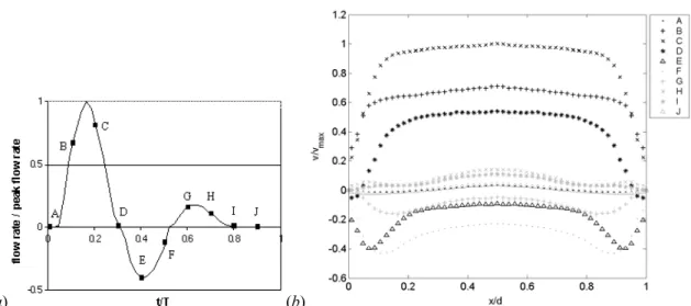
calculated based on the flow rate. The input waveform of the flow rate, non-dimensionalized by the systolic peak, is plotted in Figure 3.1 (a).
(a) (b)
Figure 3.1: (a) Flow waveform input in the pump, non-dimensionalized by the peak flow
rate Qp, (b) corresponding velocity profiles across the abdominal aorta,
non-dimensionalized by the velocity based on Qp, at different instants of time in one cardiac
cycle. The y-axis is along the symmetry axis of the model and the x-axis is in the
transverse direction.
The time evolution of the velocity field was measured in the central axial plane of the tube using the PIV system. The measurements were done zooming in on only half the vessel in order to achieve a high spatial resolution (mesh size 0.019d × 0.019d). Figure 3.1 (b) shows, at 10 representative instants of time in the cardiac cycle, the profiles of the
longitudinal velocity, v, phase-averaged over 6 cardiac cycles. At the beginning of the
cycle, the fluid is almost at rest (Figure 3.1 (b) A). During the acceleration portion of the
systole (Figure 3.1 (b) B), the flow develops into the characteristic top-hat velocity
profile. When the Womersley number is small, viscous forces dominate and the velocity profiles are parabolic in shape. However, for Womersley number above 10, which is the case in the abdominal aorta, the unsteady inertial forces dominate, and the flow is nearly top hat with thin boundary layers. At the peak systole, the thickness of the boundary layer scales as d/α. After the peak systole, the flow decelerates first along the walls and quickly
reverses, while the bulk of the fluid still moves forward, with a blunt velocity profile (Figure 3.1 (b) D). The bulk of the flow reverses only at peak diastole (Figure 3.1 (b)
the resting period (Figure 3.1 (b) I-J), the flow relaxes to near rest before being
accelerated again at the beginning of the next cardiac cycle. It is important to point out that although the flow develops an inflexional velocity profile during diastole, it remains entirely laminar during the whole cardiac cycle. At the high values of Womersley number corresponding to these measurements, the characteristic time for the growth of the instability is much longer than the period of the pulsatility.
Wall shear stresses
The evolution of the wall shear stresses was calculated over time from the velocity measurements described above. In the case of a laminar, axisymmetric flow, the WSS is simply given by . -x v µ WSS ∂ ∂ = (3.1)
The wall shear stresses have been calculated using a linear interpolation between the velocity measurement the closest to the wall and the null velocity at the wall (see Appendix A for calculation of WSS). A linear interpolation was used in the vicinity to the wall, similarly to what is commonly used for turbulent boundary layers.
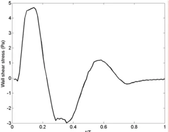
The measured temporal evolution of the wall shear stress, plotted in Figure 3.2, follows closely the evolution of the flow rate. The WSS ranges from -3 Pa to 4.9 Pa, the extrema occurring respectively at peak diastole and peak systole. The convention is to assign a negative value to WSS corresponding to reversed flow. As mentioned in Chapter 2, all the measured values correspond to the physiologically correct flow. The time-averaged WSS, , 1 0
∫
= T mean WSS dt T WSS (3.2)Figure 3.2: Wall shear stresses measured in a model of healthy infrarenal aorta.
is measured to be equal to 0.27 Pa, T being the period of the cardiac cycle. The time-average of the magnitude of the shear stress,
, 1 0
∫
= T mag WSS dt T WSS (3.3)is equal to 1.5 Pa. The oscillating shear index, , 1 2 1 ⎟ ⎟ ⎠ ⎞ ⎜ ⎜ ⎝ ⎛ − = mag mean WSS WSS OSI (3.4)
is equal to 0.4. This index quantifies the pulsatility of the flow and the main direction of the flow. It ranges from 0 (forward flow throughout the cardiac cycle) to 1 (fully reversed flow). An OSI index of 0.5 corresponds to a pure oscillating flow with a WSSmean of 0.
Oyre et al. (1997) measured the wall shear stresses along the suprarenal and infrarenal portions of the aorta in vivo and non-invasively using magnetic resonance velocity mapping. They found WSS of comparable magnitude to our experiments (-1.3 Pa ≤ WSS ≤ 4.9 Pa). From their curve of WSS, one can calculate an OSI index of 0.32. Cheng, Parker & Taylor (2002) and Taylor et al. (2002) did similar measurements with cine phase-contrast magnetic resonance imaging. But, in the case of a patient at rest, they only measured a peak wall shear stress of 2 Pa and a time-average of 0.16 Pa. Their lower
WSS values may be accounted for by the low spatial resolution of their measurements, which only allowed them to measure the velocity at 7 locations across the vessel. A higher resolution is needed to get a good estimate of the gradient of the velocity at the wall.
2. Analytical solution of the flow in a healthy abdominal aorta Hemodynamics
As a first approximation, the healthy abdominal aorta can be modeled as a straight infinite rigid tube. The flow of a viscous fluid in an infinite tube under a periodic pressure gradient was first studied by Richardson & Tyler (1929). Womersley (1954) and Helps & McDonald (1954) calculated analytical solutions for the arterial pulsating flow expressing the time-varying pressure gradient as the Fourier series of sinusoidal modes (see also Pedley 1979).
In a tube with large L/d ratio, the radial motion of the liquid can be neglected and the longitudinal velocity v is independent of the distance y. The continuity equation is then identically satisfied. The y- and r-momentum equations that govern the arterial flow can be written in the following non-dimensionalized form
, r v r r r Re y p t v Re α2 ⎟⎟ ⎠ ⎞ ⎜⎜ ⎝ ⎛ ∂ ∂ ∂ ∂ + ∂ ∂ − = ∂ ∂ ∗ ∗ ∗ ∗ ∗ ∗ ∗ ∗ ∗ 1 (3.5a) , r p 0 = ∂ ∂ ∗ ∗ (3.5b) in which the longitudinal velocity v(r, has been non-dimensionalized by U, the lengths t) r and y by the radius of the aorta a0 (a0 = d/2), the time t by the pulsation frequency ω
and the pressure p by ρU2. The stars indicate the dimensionless variables.
The pressure gradient, which is only a function of time (equation (3.5)), can be expressed as a Fourier series with constant coefficients
. 0 ∗
∑
∞ = ∗ ∗ ∗ − = ∂ ∂ int n n e G y p (3.6) We seek for solutions for the longitudinal velocity under the form of a Fourier series. The solution to equation (3.4) that satisfies the no-slip boundary condition at the walls is(
)
, ) ( ) ( 1 0 3/2 2 / 3 0 2 ∗∑
∞ = ∗ ∗ ∗ ∗ ∗ ∗ ∗ ⎟⎟ ⎠ ⎞ ⎜⎜ ⎝ ⎛ − + − = int n n n n n 2 0 e α i J α i r J 1 α G i Re r 1 4 ReG ) ,t (r v (3.7)where J0 is the Bessel function of the first kind of order 0 and αn = a0 nω/ν . One can remark that α1 = a0 ω/ν is the Womersley number α previously defined. It is interesting to notice that the time-average term of the Fourier decomposition takes the form of a Poiseuille flow induced by the mean pressure gradient ∗
0
G .
The velocity profile corresponding to our measurements can be calculated applying the conservation of mass at each instant of time. The input flow rate is
(
( ))
, 8 π π 1 2 ∗∑
∞ = ∗ ∗ ∗ ∗ ∗ ∗ = = + − int n n n n 0 1 F α e iα ReG ReG ) (t v ) (t Q (3.8)where v∗ is the instantaneous velocity, space-averaged over the tube cross-section and . ) ( ) ( 2 ) ( 3/2 0 2 / 3 1 2 / 3 n n n n α i J α i J α i α F = (3.9)
In order to analyze the above measurements, the input flow rate supplied to the vessel model in our experiment, Q∗(t∗) is decomposed into a Fourier series. The Fourier coefficients of the pressure gradient, ∗
n
G , are calculated using equation (3.8) and the
velocity profile, v∗(r∗,t∗) is then computed from equation (3.7).
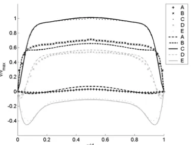
Figure 3.3 compares the PIV measurements of the phase-averaged velocity profiles across the abdominal aorta with the profiles predicted by the above Womersley solution for the same flow conditions. The comparison requires changing the variables from the Cartesian coordinate system (x, y) used in the experiment to the cylindrical coordinate system (r, y) used in the analytical solution. This change is valid as long as the
measurements are made in the central axial plane of the model and three-dimensional effects can be neglected. The difference between the experimental and the theoretical profiles is found to be about 8%, whereas the standard deviation between the 6 independent realizations that have been used to compute the average is 3.7%. The agreement between the measured velocity field and the theoretical laminar profile confirms the standard result that although the velocity profile is highly inflectional after the peak systole, the unsteadiness of the flow prevents the instability from developing.
Figure 3.3: Comparison of the velocity profiles across the abdominal aorta measured experimentally with the ones calculated with the Womersley solution.
The differences between the measured and the theoretical profiles may be a consequence of the assumptions used in the analytical model, such as the infinite vessel size. The analytical solution assumes the flow to be fully developed, whereas it may not be quite the case experimentally, since the model of AAA is located only about 20 diameters downstream of the pump. In the experiment, a difference may exist between the output wave profile from the pump and the effective waveform that enters the model. This could be either due to an inaccuracy of the pump or to modifications of the waveform between the outlet of the pump and the model due to entrance effects or to a
weak pressure peak damping. However, it is important to notice, in Figure 3.3, that the first measurement point closest to the wall is almost placed on the theoretical curve at each time step. This should guarantee a good measurement of the wall shear stress.
Wall shear stresses
The wall shear stress can be calculated from the velocity field given in equation e α F ReG ReG r v ) (t WSS int n n n 0 r . ) ( 2 2 1 1 ∗ ∗
∑
∞ = ∗ ∗ = ∗ ∗ ∗ ∗ = + ∂ ∂ − = (3.10)The computed time variation of the wall shear stress corresponding to the flow rate used experimentally (Figure 3.1 (b)) is shown in Figure 3.4.
Figure 3.4: Profile of wall shear stresses calculated with the analytical solution in a healthy abdominal aorta over one period.
The theoretical solution predicts a peak WSS of 4.87 Pa, WSSmean = 0.16 Pa, WSSmag =
1.3 Pa and OSI = 0.42, which is in good agreement with the measured values, apart from the mean value that is too low. When compared with the WSS profile measured experimentally (Figure 3.2), one can observe a good agreement. The theory, however, predicts a larger slope between the systolic and diastolic peaks. Two explanations may account for this difference in shape. In the experiment, the high frequencies may be
damped, causing a broader systolic peak. The analytical solution may also not correspond to the experimental testing conditions, the assumptions of an infinitely long, rigid model being not satisfied experimentally.
The WSS is the parameter that is physiologically relevant at the level of the endothelial cell response. This section has shown that the WSS fluctuates significantly in a healthy abdominal aorta, where the OSI parameter can be between 0.32 and 0.42. As discussed in the introduction, any departure from the healthy pattern of WSS strongly affects the morphology, metabolism and gene expression of the endothelial cells. In the next section, we will analyze how the presence of an AAA influences the spatial and temporal distribution of WSS.
D. Flow in abdominal aortic aneurysms
1. Results of the parametric study of the flow characteristics in AAA Typical flow in an aneurysm
Before analyzing the effect of aneurysmal growth on the flow topology, we will discuss the important spatial and temporal features, which characterize the typical flow field in an abdominal aortic aneurysm. For that purpose, we have selected an aneurysm with a dilatation ratio D/d = 1.9 and an aspect ratio L/d = 2.9 (model 4). The velocity field was measured in a central axial plane of the aneurysm with the PIV system with a mesh size of 0.068d × 0.068d. The vorticity and total stresses were calculated from the velocity field. The total stress is defined as the maximum eigenvalue of the stress tensor (see Appendix B) and is therefore a good measure of the maximum strain rate developing in the flow. It is important to understand how the vorticity and stresses evolve over time inside the aneurysm, since the changes in the wall shear stresses are directly related to them.
A B C D
E F G H
I J K
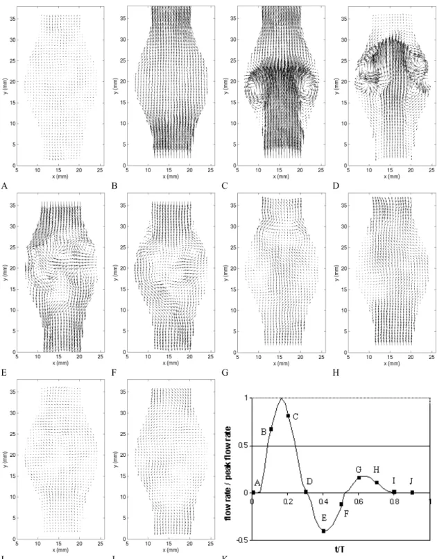
Figure 3.5: Instantaneous velocity field measured in model 4 (D/d = 1.9, L/d = 2.9) with the PIV system.
1 1 -1 (a) B C D E 0 (b) B C D E
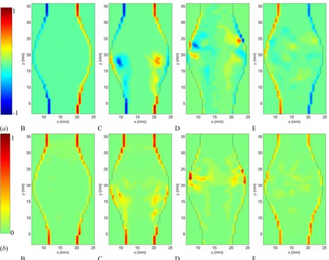
Figure 3.6: (a) Instantaneous vorticity and (b) stress fields measured in model 4 (D/d = 1.9, L/d = 2.9) at times B to E, non-dimensionalized by the peak value occurring in the healthy vessel.
During the acceleration portion of the systole, the flow remains laminar and fully attached to the bulging walls (Figures 3.5 and 3.7 (a) A-B). The fact that the flow remains attached in the divergent portion is a consequence of the positive pressure gradient generated at the beginning of the systole: the temporal acceleration of the flow is at this point larger than the convective deceleration originated by the upstream (proximal) diverging walls of the artery. Figure 3.6 B shows that, during the entire acceleration portion of the cardiac cycle, the vorticity and stresses are confined to very thin Stokes layers and the bulk of the flow behaves as a potential flow (irrotational and inviscid).
1 1 (a) B C D E -1 (b) B C D E 0 (c) B C D E
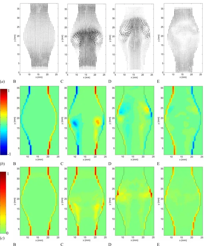
Figure 3.7: (a) Velocity, (b) vorticity and (c) stress fields, at times B to E, measured in model 4 (D/d = 1.9, L/d = 2.9) and phase-averaged over 6 cardiac cycles. The vorticity and stress fields are non-dimensionalized by the peak values occurring in the healthy vessel.
Just after the initiation of the flow deceleration (Figures 3.5 and 3.7 (a) C), one can notice the sudden reversal of the velocity field close to the wall, while the bulk of the flow is still moving forward. At this point, the flow detaches from the proximal neck. Downstream of the flow separation, the flow remains laminar and attached to the wall. The vorticity field (Figures 3.6 (a) and 3.7 (b) C) shows the roll up of the Stokes layer into a large start-up vortex. This intense vortex is followed by a free shear layer, in which some secondary vortices form due to the Kevin Helmholtz instability. The effect of flow separation is also to displace the peak of shear stresses from the wall into the bulk of the flow (Figures 3.6 (b) and 3.7 (c) C). The wall is now dominated by very low values of shear stresses, with the exception of a small portion, where the WSS is of opposite sign because of the passage of the start-up vortex very close to the wall. The vortex ring leads to a local marked increase in the wall shear stresses.
(a) (b) (c)
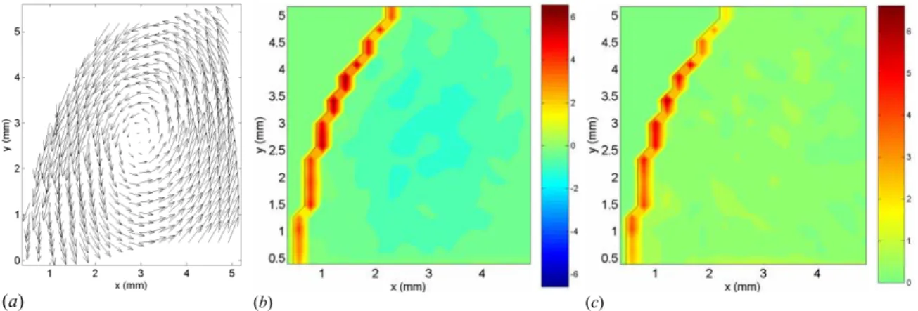
Figure 3.8: Zoom measurements of the velocity (a), vorticity (b) and stress (c) fields in the distal area of model 4 (D/d = 1.9, L/d = 2.9). The vorticity and stress values are the ones corresponding to the physiologically correct flow in SI units.
The vortex ring travels along the aneurysm until it impinges on the distal neck of the AAA (Figures 3.5 and 3.7 (a) D), resulting in a sharp increase in wall shear stresses in the converging portion of the AAA. At this point, the cylindrical internal shear layers span across the entire length of the AAA (Figure 3.6 (a) D) and the flow is fully detached from the wall along the entire AAA length. At the point of impact, the Stokes layer is
again characterized by vorticity and stresses of the opposite sign, because of the presence of the vortex ring.
(a) C D
(b) C D
Figure 3.9: Instantaneous (a) and phase-averaged (b) velocity field measured in the transverse cut located at the point of maximum diameter at times C and D.
However, the characteristic length scale of the Stokes layer becomes so small that the resolution is not sufficient to provide a reliable measurement of the flow characteristics very close to the wall at time D. Therefore, we measured the flow field in model 4, zooming in on the region near the distal wall, in order to increase the resolution (mesh size 0.027d × 0.027d). Figure 3.8 shows the velocity, vorticity and stress fields at time D. The measurements show the primary vortex ring hitting the distal wall. On the vorticity plot (Figure 3.8 (b)), one can observe the change in sign of vorticity as one moves from
the centerline to the wall passing through the vortex ring. The presence of high velocity so close to the wall induces very thin Stokes layers (≅ 0.02d) with high stresses (≥ 6 Pa). Unfortunately, the resolution is still not high enough to resolve the Stokes layer. The measured wall shear stress is therefore still underestimated.
A loss of the two-fold symmetry can be observed on the instantaneous fields as the vortex hits the wall. It corresponds to a loss in axisymmetry, which increases strongly after the vortex ring has hit the distal wall (times E and F). The resulting flow presents a larger randomness, which can be noticed when comparing the instantaneous and phase-averaged fields (Figures 3.5 and 3.6 with 3.7). It is particularly noticeable on the velocity vector plots (Figure 3.5). As the flow reverses in the diastole, the coherent shear layer and the preceding vortex ring break down leading to disordered vortices of decreasing intensity (Figures 3.5 and 3.6 E-F). Even if the Reynolds number is moderate and the range in scale of energetic vortices limited, we will call this stage a weak turbulence. In order to quantify the non-axisymmetry, we measured the velocity field in transverse planes of the AAA. Figure 3.9 shows both the instantaneous and phase-averaged velocity fields measured in the transverse cut located at the point of maximum diameter. At time C, the core of the vortex ring is located right upstream of the measurement plane. The vortex ring must be slightly inclined, since high outward velocity vectors are measured at the center of the aneurysm. However, at time D, a negative radial velocity field is induced at the rear of the vortex ring. Figure 3.9 shows that the loss of symmetry has already occurred at time C.
Near the end of the cardiac cycle corresponding to the resting period of the heart (Figure 3.5 G-J), the turbulence weakens due to vortex entanglement (energy cascade) and viscous dissipation and the flow relaxes back to a near stagnant state. At the beginning of the next cycle, some weak perturbations persist from the dissipated
turbulence. The initial flow conditions are therefore not perfectly identical for each cycle, and a small cycle-to-cycle variation is observed in our measurements.
Effect of the dilatation parameter
In order to assess the effect of the dilatation ratio on the flow topology, the flow field in the decelerating portion of the systole is plotted on Figure 3.10 for 3 comparable models. Models 1, 2 and 5 have the same aspect ratio as model 4, L/d = 2.9, but their dilatation ratio increases linearly with the model number (see Table 2.I). The corresponding vorticity fields are shown on Figure 3.10.
(a) C D (b) C D
(c) C D
Figure 3.10: Comparison of the phase-averaged velocity field measured with the PIV system in models 1 – D/d = 1.3 (a), 2 – D/d = 1.5 (b) and 5 – D/d = 2.1 (c) at times C and D. A small phase-lag between the different experiments is possible, since the frequency
of acquisition of the measurements is a harmonic of the frequency of the flow, but the relative phase between experiments varies
(a) C D (b) C D
(c) C D
Figure 3.11: Comparison of the phase-averaged vorticity field measured in models 1 –
D/d = 1.3 (a), 2 – D/d = 1.5 (b) and 5 – D/d = 2.1 (c) at times C and D,
non-dimensionalized by the peak value occurring in the healthy vessel.
It is remarkable that the clinically relevant features of aneurysmal flows, i.e. detachment of the flow and impingement on the distal neck, occur even for a dilatation parameter as low as 1.3 for short aneurysms (Figures 3.10 (a) and 3.11 (a)). Even an incipient aneurysm is characterized by the formation of recirculating zones close to the wall. We can notice that the flow separation occurs around the peak systole in all of the models (between times B and C in Figures 3.10 and 3.11). The time, at which flow separation occurs, does not seem to depend on the dilatation parameter, contrary to the point of flow separation. As the aneurysm grows in size, the point of flow separation gets
1
closer to the proximal neck. The size of the detached flow region also increases as the dilatation parameter is increased. When D/d increases, the detachment becomes more massive and a larger vortex ring is generated. A shear instability length scale can be observed in the shear layer for the small dilatation ratio models. It is of the order of the vessel radius a (Figure 3.10 (a) and (b)). It is, however, impossible to conclude whether this length scale is the primary one or whether vortex pairing has already occurred.
(a) C D (b) C D
(c) C D
Figure 3.12: Comparison of the phase-averaged velocity field measured in models 11 –
L/d = 5.2 (a), 6 – L/d = 3.9 (b) and 1 – L/d = 2.9 (c) at times C and D.
Effect of the aspect ratio
Figure 3.12 features the effects of decreasing the aspect ratio on the phase-averaged velocity fields at times C and D (models 11 – L/d = 5.2, 6 – L/d = 3.9 and 1 – L/d = 2.9).
The models have decreasing aspect ratios, but they all have the same dilatation ratio (D/d = 1.3). Figure 3.13 shows the corresponding contours of the phase-averaged vorticity.
(a) C D (b) C D
(c) C D
Figure 3.13: Comparison of the phase-averaged vorticity field measured in models 11 –
L/d = 5.2 (a), 6 – L/d = 3.9 (b) and 1 – L/d = 2.9 (c) at times C and D,
non-dimensionalized by the peak value occurring in the healthy vessel.
A first striking difference is the length traveled by the vortex ring. This length, l, measured as the greatest distance between the core of the vortex ring and the proximal neck, was plotted on Figure 3.14 for the different values of L/d and D/d ratios.
The ratio l/d is to be compared with the Strouhal number calculated with the systolic time tsyst (Gharib, Rambod & Shariff 1998; Stroud, Berger & Saloner 2000)
1
d t U St syst syst
syst = . (3.11)
This Strouhal number is the controlling parameter of the vortex shedding. A characteristic systolic velocity can be chosen as half the peak velocity, which would correspond to an average systolic velocity. The Strouhal number is then found to equal to
. 3 16 . 0 π 4 2 1 2 = = d T d Q St p syst (3.12)
since the systolic time is about 16% of the cardiac period T. One can see that l/d tends to
Stsyst, as D/d increases. However the aspect ratio of the model may limit the evolution of
the vortex ring, when the length available to the vortex ring to propagate is less than 3d, as seen for L/d = 2.9. In the models with L/d = 2.9, the core of the vortex ring do not go beyond y/d = 2.3, which corresponds to the location of the point of impingement on the distal wall. Apart from the case of small aspect ratios, where L/d becomes a limiting parameter, the length traveled by the vortex ring inversely scales with L/d.
Figure 3.14: Maximum position of the core of the vortex ring inside the AAA plotted as a function of the D/d and L/d ratios.
The second difference is the time at which flow separation occurs in the cycle. Whereas the flow separates around the peak systole for L/d = 2.9 (model 1) (between times B and C on Figures 3.12 (c) and 3.13 (c)), the separation is delayed to time C for
L/d = 3.9 (model 6) (Figures 3.12 (b) and 3.13 (b)) and even further to time D for L/d = 5.2 (model 11) (Figures 3.12 (a) and 3.13 (a)). Since the separation occurs later in the deceleration phase for higher aspect ratios, the generated vortex ring has a reduced strength. This implies that longer aneurysms are less pathological than short ones. An increased length delays the appearance of "disturbed flow" conditions and drastically reduces the magnitude of the vortex strength. As far as the geometrical parameters are concerned, these results correlate well with the ones found by Hatakeyama, Shigematsu & Muto (2001), who characterized the risk factors for rupture as the diastolic pressure, the ratio D/L and the expansion rate of the maximum diameter.
2. Results of the parametric study of the wall shear stresses in AAA Comparison of the WSS in a typical AAA with the reference case
We discuss here the results of the parametric study, concentrating now on the spatial and temporal changes in wall shear stresses, which occur as the AAA enlarges. We shall first present the results obtained in model 4 (D/d = 1.9, L/d = 2.9) to analyze the general changes that occur in a typical established aneurysm as compared to a healthy abdominal aorta. The effects of the dilatation parameter and aspect ratio will then be discussed in the following subsections.
The wall shear stresses are defined as
, ). . ( 2µ σn t WSS = r r (3.13)
nr and tr being respectively the normal and tangential unit vectors and ]
[ 2
1µ u uT
the rate of deformation tensor for a Newtonian fluid.
(a) (b)
(c) (d)
Figure 3.15: Time evolution of the non-dimensionalized, phase-averaged wall shear stresses along the aneurysmal wall in models 1 – D/d = 1.3 (a), 2 – D/d = 1.5 (b), 4 – D/d = 1.9 (c) and 5 – D/d = 2.1 (d). y/d = 0 is located at the proximal neck for each of the models. On the time scale, t/T = 0.1 corresponds to time A, t/T = 0.2 to time B, etc.
The phase-averaged WSS, non-dimensionalized by the peak WSS, is shown in Figure 3.15 (c) for the case of model 4. In the systole (t/T = 0.2), the WSS decreases as the local diameter increases. The WSS follows a similar trend as the velocity, which inversely scales with the diameter in order to conserve mass. This is due to the fact that the flow is fully attached to the walls at systole. At t/T = 0.3, the flow detaches from the proximal neck (y/d = 0) creating a region of zero WSS between 0 ≤ y/d ≤ 0.8. The region of large
negative WSS around y/d = 1.2 is due to the presence of the core of the large primary vortex ring. At t/T = 0.4, the vortex has traveled to y/d = 2.1, but the fact that the measurements are taken at discrete times prevents us from following the vortex ring more closely during its evolution through the AAA. At t/T = 0.4, the vortex ring impinges on the distal wall. However, as discussed in the previous subsection, the WSS value is underestimated at the point of impact, because of the very small size of the Stokes layer and of the resolution of our measurements. Furthermore, the presence of the primary vortex ring so close to the wall induces the roll-up of the Stokes layer into a counter-rotating vortex of smaller size, which can be observed at y/d = 1.5, t/T = 0.4. Upstream of it, the wall still experiences very low WSS (WSS ≅ 0). At the end of the diastole as well as in the resting period of the cycle, the walls of the entire aneurysm are dominated by very low WSS.
The gradients of the phase-averaged WSS are plotted on Figure 3.16 (c). Strong gradients are observed at the proximal and distal necks at times t/T = 0.2, when the changes in WSS are maximum at the necks and t/T = 0.3, when the flow detaches in the aneurysm. The formation of the vortex ring also induces very strong gradients just upstream and downstream of it (t/T = 0.3-0.4). The locations of these regions of high gradients therefore move along with the vortex ring, affecting different parts of the wall over time. But the time, when most of the aneurysm wall experiences strong gradients, occurs after the flow massively detaches from the wall (t/T = 0.3).
(a) (b)
(c) (d)
Figure 3.16: Time evolution of the gradient of the phase-averaged wall shear stresses along the aneurysmal wall in models 1 – D/d = 1.3 (a), 2 – D/d = 1.5 (b), 4 – D/d = 1.9 (c) and 5 – D/d = 2.1 (d), measured in N/m3. y/d = 0 is located at the proximal neck for each of the models. On the time scale, t/T = 0.1 corresponds to time A, t/T = 0.2 to time B, etc.
The WSSmean, as defined in section C.1 along with WSSmag and the OSI index, sharply
drops after the proximal neck to almost zero and remains very low between 0.1 ≤ y/D ≤ 0.7. This can be seen on Figure 3.17 (c), which shows the WSSmean for model 4. The WSSmean then reaches higher negative values, the negative peaks correlating with the
presence of the vortex ring, respectively at times t/T = 0.3 and 0.4. One can observe that,
on average, most of the aneurysm wall is subjected to negative WSSmean of small
(a) (b)
(c) (d)
Figure 3.17: Evolution of WSSmean along the aneurysmal wall in models 1 – D/d = 1.3 (a),
2 – D/d = 1.5 (b), 4 – D/d = 1.9 (c) and 5 – D/d = 2.1 (d). The results are shown only inside the AAA.
The WSSmag decreases in the proximal half and increases back in the distal half with
some fluctuations (see Figure 3.18 (c)). One can notice that the values of the healthy vessel are not met at the proximal neck but further upstream, at y/d = -0.4. The presence of the aneurysm partly disrupts the flow at the entrance vessel close to the neck.
(a) (b)
(c) (d)
Figure 3.18: Evolution of WSSmag along the aneurysmal wall in models 1 – D/d = 1.3 (a),
2 – D/d = 1.5 (b), 4 – D/d = 1.9 (c) and 5 – D/d = 2.1 (d).
The OSI index points out the regions of oscillatory flows (OSI ≅ 0.5) as well as the regions of mean forward (OSI < 0.5) or reversed (OSI > 0.5) flow. The region of very low
WSSmean observed in model 4 (0.1 ≤ y/d ≤ 0.7) is characterized by an OSI index close to
0.5 (Figure 3.19 (c)). In the regions of high negative WSSmean, the OSI index further
increases to reach 0.8 over a large portion of the AAA (1.3 ≤ y/d ≤ 2.2). Most of the aneurysm wall experiences an OSI index larger than 0.5, which shows that reversed flow conditions are dominant.
(a) (b)
(c) (d)
Figure 3.19: Evolution of the OSI factor along the aneurysmal wall in models 1 – D/d = 1.3 (a), 2 – D/d = 1.5 (b), 4 – D/d = 1.9 (c) and 5 – D/d = 2.1 (d).
Effect of the dilatation parameter on the WSS
In the systole, the decrease of the WSS becomes more pronounced with increasing
D/d ratio. This can be observed, when comparing the plots of wall shear stresses for models 1, 2, 4 and 5 shown in Figure 3.15. Also, as D/d increases, the point of flow separation gets closer to the proximal neck (y/d = 0.8 for D/d = 1.3 (model 1) to be compared to y/d = 0.1 otherwise). So the WSSmean drops more abruptly to near zero values
as D/d increases (Figure 3.17). The third important effect of the dilatation ratio concerns the size of the detached region. The recirculation region is seen to increase with D/d,
increasing from a length equivalent to 1d for D/d = 1.3 (model 1), to 2d for D/d = 1.5 (model 2), to the whole length of the aneurysm (2.8d) for D/d = 2.1 (model 5). The increase in the size of the detached region leads to an increase in the section of the vessel wall subjected to a reversed flow, characterized by a negative mean WSS (Figure 3.17) and an OSI index greater than 0.5 (Figure 3.19). The accentuation of the drop in WSS in the systole and the increase in size of the regions subjected to very low WSS are responsible for the gradual decrease in WSSmag as D/d increases (Figure 3.18). The
average value of the WSSmag inside the AAA drops from 1.1 Pa for D/d = 1.3 (model 1),
to 0.75 Pa for D/d = 1.5 (model 2), to 0.60 Pa for D/d = 1.9 (model 4) and finally to 0.37 Pa for D/d = 2.1 (model 5). The decrease in WSSmag causes an increase in the maximum
value of the OSI index (Figure 3.19), so that the index average value dramatically increases as D/d increases. The dilatation ratio does not seem to influence the amplitude of the negative WSS at the location of the vortex ring.
Effect of the aspect ratio on the WSS
For a same dilatation parameter D/d, the main effect of increasing the aspect ratio of the aneurysm is to make all the above described changes in the patterns of WSS less pronounced. Figure 3.20 shows the spatial and temporal evolution of the WSS in models 11, 6 and 1, which have a dilatation ratio of 1.3 and decreasing aspect ratios (5.2, 3.9 and 2.9). In the systole, the effect of the dilatation is visible for all the models. Note that, even in model 11, the increase in diameter leads to a decrease in WSS.
(a) (b)
(c) Figure 3.20: Time evolution of the non-dimensionalized, phase-averaged wall shear
stresses along the aneurysmal wall in models 11 – L/d = 5.2 (a), 6 – L/d = 3.9 (b) and 1 –
L/d = 2.9 (c). y/d = 0 is located at the proximal neck for each of the models. On the time scale, t/T = 0.1 corresponds to time A, t/T = 0.2 to time B, etc.
As L/d increases, the flow separation is delayed, as shown in Figure 3.20. It is observed to occur only at t/T = 0.3 for L/d = 3.9 (model 6) and at t/T = 0.4 for L/d = 5.2 (model 11). The vortex ring, generated at a later time in the cardiac cycle, is therefore weaker in intensity, inducing smaller negative WSS. The delay of the flow separation to instants when the WSS are smaller and the decrease in intensity of the vortex ring are the reasons for the very large decrease in WSS gradients measured as L/d increases (Figure 3.21). Note that, in model 11, the GWSS drop to negligible values (Figure 3.21 (a)). In
this case, the flow separation is so incipient that no appreciable vortex ring is seen forming, which explains why the WSSmean (Figure 3.22 (a)) and the OSI index (Figure
3.23 (a)) remain in the normal range measured in the healthy abdominal aorta. For the rest of the discussion, we will now set model 11 aside, since it is the only model not to exhibit the classical characteristics of the flow in an AAA.
(a) (b)
(c) Figure 3.21: Time evolution of the gradient of the phase-averaged wall shear stresses
along the aneurysmal wall in models 11 – L/d = 5.2 (a), 6 – L/d = 3.9 (b) and 1 – L/d = 2.9 (c), measured in N/m3. y/d = 0 is located at the proximal neck for each of the models. On the time scale, t/T = 0.1 corresponds to time A, t/T = 0.2 to time B, etc.
(a) (b)
(c) Figure 3.22: Evolution of WSSmean along the aneurysmal wall in models 11 – L/d = 5.2
(a), 6 – L/d = 3.9 (b) and 1 – L/d = 2.9 (c). The results are shown only inside the AAA. One can notice that the relevant parameters, such as the WSSmean or the OSI index,
have a similar variation in space for both models. The values are practically identical in
each case and the maximum in OSI or the minimum in WSSmean occur at the same
location, although the length of the models is different. This shows that the L/d parameter has little effect on the physical processes that occur inside the AAA.
(a) (b)
(c) Figure 3.23: Evolution of the OSI index along the aneurysmal wall in models 11 – L/d = 5.2 (a), 6 – L/d = 3.9 (b) and 1 – L/d = 2.9 (c).
3. Analytical solution for a slowly expanding abdominal aorta Hemodynamics
The study of the changes in the WSS resulting from very small dilatations of the abdominal aorta, prior to their development into an aneurysm, is crucial for a better understanding of the etiology of the disease. An analytical solution of the flow in an incipient aneurysm, such as the one studied in model 11 (D/d = 1.3, L/d = 5.2), would therefore be a useful tool to study the evolution of AAAs in a systematic way.
One can obtain an analytical solution for the WSS by extending the case of a straight pipe, shown in section C.2, to a slowly expanding pipe. In this case, the radial velocity,
ur(y, r, t), cannot be neglected. Using the dimensionless variables introduced in section
C.2, the equation of mass conservation can be written as
0 = ∂ ∂ + + ∂ ∂ ∗ ∗ ∗ ∗ ∗ ∗ y v r u r ur r (3.15)
and the y- and r-momentum equations as
, 1 1 2 2 2 ⎟⎟ ⎠ ⎞ ⎜⎜ ⎝ ⎛ ⎟⎟ ⎠ ⎞ ⎜⎜ ⎝ ⎛ ∂ ∂ ∂ ∂ + ∂ ∂ + ∂ ∂ − = ∂ ∂ + ∂ ∂ + ∂ ∂ ∗ ∗ ∗ ∗ ∗ ∗ ∗ ∗ ∗ ∗ ∗ ∗ ∗ ∗ ∗ ∗ ∗ r v r r r y v Re y p y v v r v u t v Re α r (3.16a) . ) / ( 1 2 2 2 2 2 ⎟⎟ ⎠ ⎞ ⎜⎜ ⎝ ⎛ ∂ ∂ + ∂ ∂ + ∂ ∂ + ∂ ∂ − = ∂ ∂ + ∂ ∂ + ∂ ∂ ∗ ∗ ∗ ∗ ∗ ∗ ∗ ∗ ∗ ∗ ∗ ∗ ∗ ∗ ∗ ∗ ∗ r r u r u y u Re r p y u v r u u t u Re α r r r r r r r (3.16b)
Let Λ be the characteristic length along which the local radius a(y) varies, i.e. Λ =
a0da/dy. We assume that the changes in the y-velocity, v∗(y∗,r∗,t∗), are small along y. We therefore introduce a new variable Y = ε∗ y , where the small parameter ε is defined ∗
as ε = Λ /a0. Furthermore, we define a new radial velocity, U , such that r∗ u = εr∗ U with r∗
∗
r
U of order 1 and a new pressure P = ε∗ p . With the introduction of these new ∗
variables, the conservation of mass and momentum equations become 0 = ∂ ∂ + + ∂ ∂ ∗ ∗ ∗ ∗ ∗ ∗ Y v r U r Ur r (3.17) , 1 1 2 2 2 2 ⎟⎟ ⎠ ⎞ ⎜⎜ ⎝ ⎛ ⎟⎟ ⎠ ⎞ ⎜⎜ ⎝ ⎛ ∂ ∂ ∂ ∂ + ∂ ∂ + ∂ ∂ − = ∂ ∂ + ∂ ∂ + ∂ ∂ ∗ ∗ ∗ ∗ ∗ ∗ ∗ ∗ ∗ ∗ ∗ ∗ ∗ ∗ ∗ ∗ ∗ r v r r r Y v ε Re Y P Y v εv r v εU t v Re α r (3.18a) . ) / ( 1 1 2 2 2 2 2 2 2 ⎟⎟ ⎠ ⎞ ⎜⎜ ⎝ ⎛ ∂ ∂ + ∂ ∂ + ∂ ∂ + ∂ ∂ − = ∂ ∂ + ∂ ∂ + ∂ ∂ ∗ ∗ ∗ ∗ ∗ ∗ ∗ ∗ ∗ ∗ ∗ ∗ ∗ ∗ ∗ ∗ ∗ r r U r U Y U ε Re r P ε Y U εv r U εU t U Re α r r r r r r r (3.18b)
Assuming α2/Re of order unity3, the leading order of equation (3.18b) leads to
∗ ∗ ∂
∂P / r = 0. At the first order, the momentum equations are decoupled and reduce to the
3 In the abdominal aorta of a healthy adult male at rest, α ≈ 10 and 〈Re〉 ≈ 300, so that α2 /Re≈ 1.
ones corresponding to the straight pipe. The dimensionless longitudinal velocity ) t , r (Y v∗ ∗, ∗ ∗ is then given by . ) ( ) / ( 1 ) ( 4 1 0 3/2 2 / 3 0 2 2 2 2
∑
∞ ∗ = ∗ ∗ ∗ ∗ ∗ ∗ ∗ ∗ ⎟⎟ ⎠ ⎞ ⎜⎜ ⎝ ⎛ − + − = int n n n n n 0 e α i J R r α i J iα R ReG r R ReG v (3.19)where R∗(Y∗)=a(Y∗)/a0 is the dimensionless local radius, α
n(Y∗) = a(Y∗) nω/ is ν
the Womersley number corresponding to the nth harmonic of the pulsation ω and G∗(Y∗) n is the nth Fourier coefficient of the pressure gradient ∂P /∗ ∂Y∗.
To achieve mass conservation, the flow rate at any location Y∗ inside the aneurysm
. )] ( 1 [ 8 2 1 2 4 4 0 ∗ ∗
∑
∫
∗ ∗ ∗ ∗ ∗ ∞= ∗ ∗ ∗ = = + − int n n n n 0 R e α F iα R πReG R πReG dr v r π Q (3.20)must be equal to the flow rate input at the pump
, ) , , 0 ( 2 1 0 ∗ ∗ ∗ ∗ ∗ ∗ ∗ = =
∫
πr v Y r t dr Q (3.21)which is only a function of time. Therefore the Fourier coefficients of the flow rate cannot depend on Y∗, which implies
= ∗ ∗R 4 G0 const, (3.22a) = − ∗ ∗ 2[1 ( )] n nR F α G const. (3.22b)
The radial velocity Ur∗(Y∗,r∗,t∗) is then calculated integrating the mass conservation equation (3.17) along with the conditions (3.22).
. ) ( ) / ( ) ( 1 ) ( 4 1 4 1 1 3/2 2 / 3 1 2 2 2 2 2 ∗
∑
∞ = ∗ ∗ ∗ ∗ ∗ ∗ ∗ ∗ ∗ ∗ ∗ ∗ ∗ ∗ ∗ ∗ ∗ ⎟⎟ ⎠ ⎞ ⎜⎜ ⎝ ⎛ − − + ⎟⎟ ⎠ ⎞ ⎜⎜ ⎝ ⎛ − = int n n n n n n 0 r e α i J R r α i J R r α F α F dY dR R ReG R r R r dY dR R ReG U (3.23)A B C D E
F G H I J
Figure 3.24: Velocity field calculated with the slowly expanding aneurysm model in an AAA with the same geometry as model 11.
From the Fourier decomposition of Q∗, one can calculate the Fourier coefficients of the pressure gradients, Gn∗(Y∗) using (3.20) and then the velocity components,
) t , r (Y
v∗ ∗, ∗ ∗ and Ur∗(Y∗,r∗,t∗), respectively from (3.19) and (3.23). Figure 3.24 shows the velocity field across a small aneurysm calculated for a slowly expanding aneurysm model with a dilatation ratio D/d = 1.3 and aspect ratio L/d = 5.2 (geometric parameters of model 11). The flow conditions are the same as the ones used experimentally.
Wall shear stresses
. ) ( 2 2 , 1 ∗ ∗ ∗
∑
∞ = ∗ ∗ = ∗ ∗ ∗ ∗ ∗ = + ∂ ∂ − = int n n n 0 R r e α F ReG ReG r v ) t (Y WSS (3.24)Figure 3.25 shows the profile of WSS calculated for an aneurysm corresponding to model 11. Note that for this incipient AAA, the WSS profile is very similar to the one measured in model 11 (Figure 3.20 (a). The only slight difference is the presence of slightly higher negative WSS at the location of the incipient flow separation (y/d = 1) in the experimental result, followed by smaller negative values of WSS associated with the separation of the shear layer from the wall.
Figure 3.25: Wall shear stresses calculated with the slowly expanding aneurysm model in an AAA with the same geometry as model 11.
E. Discussion
It has been long known that the structural function of the intimal layer of the abdominal aorta (comprising the endothelial cells) is sensitive to the local hemodynamic parameters. Experiments, in which the temporal distribution of shear stresses applied to the endothelial cells could be carefully controlled, have shown that the endothelial
behavior depends not only on the magnitude of the shear stresses but also on their spatial and temporal variations. These mechanotransduction mechanisms have been postulated to play a key role in vasoregulation and in the localization of intima hyperplasia and intima lesions in regions of “disturbed flow conditions”, i.e. regions where the WSS and GWSS differ from the healthy conditions. Thus, the characterization of the changes in the WSS resulting from the enlargement of the artery is essential to understand the etiology of AAAs as well as the role that the hemodynamics plays in its progression.
Our comparative measurements of the spatial and temporal distribution of the wall shear stresses in idealized models of AAA have shown that the flow inside the aneurysm is characterized by the formation of regions of larger and lower amplitude of wall shear stresses than in the healthy vessel, as well as regions of large gradients of wall shear stresses, which are virtually non existent in the healthy case. We have found that, even at large values of the dilatation parameter, the flow remains attached to the walls during systole as a consequence of the large systolic acceleration, typical of the flow waveform in the aorta. However, we have found that, in all cases studied, the flow detaches from the wall during the deceleration period immediately following the peak systole. A large start-up vortex forms and, as it propagates through the aneurysm, secondary vortex rings develop in the associated internal shear layers. With the exception of a small zone affected by the vortex, the vessel walls are then exposed to very low and oscillating wall shear stresses. The flow detachment and the impingement of the vortex ring on the distal end of the AAA cause the formation of regions along the wall with large spatial gradients of wall shear stresses. In addition, we have shown that a region of sustained gradients of wall shear stresses always forms for aspect ratios smaller than the systolic Strouhal number, Stsyst, when the primary vortex ring impinges on the distal end. During the
diastole, the flow reversal causes a transition to a state of weak turbulence, which is subsequently dissipated over the resting period of the cardiac cycle.
A-1 A0 A1 A2 A3 A4
y/d = -0.4 y/d = 0 y/d = 0.75 y/d = 1.5 y/d = 2.25 y/d = 3
WSSmax (N/m2) 4.5 2.8 1.2 0.8 1 3.3
WSSmin (N/m2) -2.5 -1.5 -1 -1 -2 -2
WSSmean (N/m2) 0.44 0.28 -0.09 -0.23 -0.24 0.39
WSSmag (N/m2) 1.46 0.88 0.46 0.38 0.6 1.2
OSI 0.35 0.34 0.60 0.81 0.70 0.34
Table 3.I: Comparison of different characteristic quantities, WSSmax, WSSmin, WSSmean, WSSmag and OSI, at 6 positions along the AAA in model 4 (D/d = 1.9): A-1 (y/d = -0.4), A0 (y/d = 0), A1 (y/d = 0.75), A2 (y/d = 1.5), A3 (y/d = 2.25) and A4 (y/d = 3).
These changes in the flow characteristics result in very large changes in the spatial and temporal WSS distribution acting on the endothelial cells as compared to those acting on the healthy aorta (Figure 3.4). Depending on their location along the aneurysm wall, the EC experience very different patterns of WSS and GWSS as the AAA enlarges. Our measurements show the existence of two main regions, the location and size of which change as the aneurysm grows: the detached region and the reattachment region. The first region is located approximately in the proximal half of the AAA and is dominated by a large decrease in the magnitude of the WSS, as shown in Table 3.I. The WSS profile evolves from the highly pulsatile waveform measured in the healthy vessel (y/d = -0.4) to an oscillatory waveform of small amplitude (±1 N/m2) and zero mean value near the mid-point region (y/d = 0.75) to a waveform of even smaller amplitude and negative mean at the point of maximum diameter (Figure 3.26). A peak in the GWSS occurs at the time of flow separation (Figure 3.27). However, this peak, owing to its short duration, is unlikely to have an important impact on the function of the endothelial cells.
A-1 A2
A0 A3
A1 A4
Figure 3.26: Time evolution of the wall shear stresses at a few locations inside model 4 (D/d = 1.9): A-1 (y/d = -0.4), A0 (y/d = 0), A1 (y/d = 0.75), A2 (y/d = 1.5), A3 (y/d = 2.25) and A4 (y/d = 3). One can see again the similarity between the WSS profile measured in the healthy part of the tube (A-1) with the analytical solution (Figure 3.4). One can then observe the extent of the changes in WSS inside the aneurysm, when comparing the profiles of WSS at location A0, A1, A2 and A3 with Figure 3.4.
A-1 A2
A0 A3
A1 A4
Figure 3.27: Time evolution of the gradients of wall shear stresses at a few locations inside model 4 (D/d = 1.9): A-1 (y/d = -0.4), A0 (y/d = 0), A1 (y/d = 0.75), A2 (y/d = 1.5),
A3 (y/d = 2.25) and A4 (y/d = 3).
In contrast, in the reattachment region, comprising nearly the second half of the AAA, we have measured sustained GWSS along with high negative WSS (around y/d =
2.25 in Figures 3.26 and 3.27). Our measurements show that this second region is subjected to GWSS over 70% of the duration of the cardiac cycle (Figure 3.27). Even the distal neck experiences strong fluctuating gradients. Furthermore, the impinging vortex ring produces high wall shear stresses in the reversed flow direction (negative values) at a late time in the cardiac cycle.
Our measurements of the spatial and temporal distribution of WSS could provide the basis for the design of endothelial cell experiments, where one could study their proliferation, altered gene expression, cell adhesion as well as the activation of the various biological processes under the realistic flow conditions encountered inside the AAA. These studies will greatly enhance our understanding of the role that the mechanical stimuli play in the etiology and progression of AAAs.
The flow changes reported here for symmetric AAA are expected to be even more pronounced in in vivo AAAs, since most later-stage aneurysms grow non-symmetrically, because of the presence and support of the spinal column. In the next chapter, we will show that the basic mechanisms linked to the separation of the flow at the peak systole and the roll up of the vortices are similar for non-axisymmetric AAAs. Since the vortex stretching is stronger and occurs sooner in the non-symmetric case, the turbulence is likely to be more intense. In vivo, the presence of the renal arteries and the lumbar curvature may also have an important effect on the flow and constitute a limitation of our study. The low distal impedance in the renal arteries leads to a suction effect that causes blood at the posterior wall to reverse and to flow back upstream into the renal arteries. Vortices are therefore formed at the entrance of the infrarenal aorta (Moore et al. 1992), modifying partly the flow in the parent vessel to the AAA, especially along the posterior wall. The lumbar curvature may also cause the formation of detached vortices leading to a mechanism similar to the one described here for a straight aneurysm. We can infer in both cases that the flow field may be phenomenologically similar as far as flow
separation, vortex roll up, vortex impingement on the wall as the one we conducted. Therefore, although this study was conducted in simplified models of AAA, it captures all the critical flow changes that occur once an aneurysm forms, and provides a much needed tool to analyze quantitatively the effects of the modifications in the mechanical stimuli on the formation and growth of AAAs.
F. Conclusion
We have measured systematically the effects of the growth of AAAs on the spatial and temporal distribution of the wall shear stresses. Measurements conducted in rigid symmetric AAA models have shown that flow separation occurs even at very early stages during the AAA formation (D/d ≥ 1.3). The flow separation and the associated formation of a strong vortex ring and of internal shear layers lead to regions of perturbed stress distribution, which do not exist in a healthy abdominal aorta. For all the aneurysm models characterized by a dilatation ratio greater than 1.5, the mean WSS consistently drops from the healthy aorta value of 0.40 N/m2 to values very close to zero, when averaged over the whole aneurysm length. However, the decrease in the average magnitude of the WSS becomes larger as the dilatation ratio increases.
In terms of WSS patterns, two main regions were identified, the detached region and the reattachment region, the size and location of which change as the aneurysm grows. On the one hand, the detached region, located in the proximal half of the aneurysm, is dominated by oscillatory wall shear stresses of very low, negative WSSmean. A very large
peak in the GWSS occurs at the location and time of flow separation and reaches about −600 N/m3. But the gradients remain otherwise quite small in the proximal half.
On the other hand, the region of flow reattachment is characterized by large, sustained GWSS and large negative WSS. Most of the distal wall is subjected to GWSS
values occurring upstream and downstream of the traveling vortex ring. Simultaneously, the WSSmean, negative over the entire distal half of the AAA, reaches -0.4/-0.5 N/m2 and
the OSI index a maximum of 0.8 in the region of impact of the vortex ring.
Further studies of endothelial cell subjected to the specific spatial and temporal distribution of WSS and GWSS reported here should provide the necessary information, in order to elucidate the possible role that these disturbed patterns of WSS may have on the etiology and progression of AAAs.