HAL Id: tel-01735046
https://pastel.archives-ouvertes.fr/tel-01735046
Submitted on 15 Mar 2018HAL is a multi-disciplinary open access archive for the deposit and dissemination of sci-entific research documents, whether they are pub-lished or not. The documents may come from teaching and research institutions in France or abroad, or from public or private research centers.
L’archive ouverte pluridisciplinaire HAL, est destinée au dépôt et à la diffusion de documents scientifiques de niveau recherche, publiés ou non, émanant des établissements d’enseignement et de recherche français ou étrangers, des laboratoires publics ou privés.
Motion analysis for Medical and Bio-medical
applications
Élodie Puybareau
To cite this version:
Élodie Puybareau. Motion analysis for Medical and Bio-medical applications. Bioinformatics [q-bio.QM]. Université Paris-Est, 2016. English. �NNT : 2016PESC1063�. �tel-01735046�
Université Paris-Est
Laboratoire d’Informatique Gaspard Monge (LIGM)
∗∗∗
Thesis submitted as requirements for the degree of doctorate in
computer science of Université Paris-Est
∗∗∗
Elodie Puybareau
∗∗∗∗∗
Motion analysis for Bio-medical
applications
∗∗∗∗∗
Toru Tamaki
Rapporteur
Jesus Angulo
Rapporteur
Olivier Meste
Examinateur, Président du Jury
Caroline Chaux
Examinateur
Pierre-Régis Burgel Examinateur
Hugues Talbot
Examinateur
Laurent Najman
Directeur
André Coste
Co-Directeur
Acknowledgements
I would like to warmly thank Jesus Angulo and Toru Tamaki who accepted to review this manuscript. I also want to thank Olivier Meste, Caroline Chaux and Pierre-Régis Burgel who accepted to be the examiners of my thesis.
Un manuscrit de thèse, c’est l’aboutissement d’une parenthèse de vie. Une sorte de marathon, lien entre les études et le monde du travail, la découverte du monde de la recherche dans lequel on plonge sans trop savoir ce qu’on va y trouver. Je termine mon manuscrit par les remerciements, dernière page que j’écrirai, et la plus dure. On pourrait croire que les remerciements ne sont qu’une formalité. Ce n’est pas le cas. Comment transmettre 3 ans de larmes et de rires, de prises de tête et de consensus, de conversations animées et de calme bienfaiteur, qui ont permis de faire naître de nouvelles idées et d’afûter mon esprit (et, soyons honnêtes, de survivre à ces 3 années nerveusement pas toujours simple) ?
Comme à la fin d’un bon roman, on dit au revoir aux protagonistes, on referme le livre pour passer à autre chose. Bien sûr, l’histoire continue, mais le décor est différent, c’est un nouveau tome qui commence dans lequel les rôles ont évolué. Cher lecteur, comme lors d’une cérémonie des oscars, je vais citer de nombreuses personnes (même le chat!), que vous ne connaissez probablement pas, mais comme à cette cérémonie, c’est le passage obligé (vous pouvez aussi tourner la page et continuer votre lecture).
Par où commencer ? Par le plus récent peut-être, en remerciant mon jury, mes rapporteurs Jesus Angulo et Toru Tamaki qui ont accepté de rapporter mon manuscrit ainsi que mes examinateurs, Olivier Meste, Caroline Chaux et Pierre-Régis Burgel. Vous m’avez tous permis d’avoir des discussions pertinentes et ainsi donné des pistes d’amélioration. Merci pour le temps que vous m’avez consacré. J’aimerais aussi remercier toute l’équipe de Créteil qui m’a adoptée pendant ces 3 ans. Merci à Estelle Escudier, Bruno Louis, Emilie Bequignon, Gabriel Pelle, Mathieu Bottier, Jean-François Papon, André Coste pour leurs conseils et leur aide, pour le temps que chacun a pu passer avec moi que ce soit pour les manips ou les discussions. Merci à toi André, d’avoir été mon directeur de thèse, d’avoir esayé de rentrer dans mon monde et de m’avoir ouvert la porte du tien. J’ai un remerciement tout particulier à faire aussi à Gabriel. Merci d’avoir cru en moi, et de
m’avoir accompagnée depuis avant l’ISBS jusqu’à la fin de ma thèse, soit pendant 6 ans. Merci de m’avoir offert ces opportunités, que ce soit à l’ISBS, au service d’explorations fonctionnelles ou avec la thèse.
Merci à Alexandra de Tassigny, à la fois à l’ISBS quand j’étais étudiante mais aussi "enseignante" (et de m’avoir fait confiance dans ce rôle là), et de m’avoir aidée pendant la thèse à réaliser une expérience des plus importante (décrite dans le manuscrit, vous la découvrirez plus tard...).
Merci aux personnes “administratives”, en particulier Sylvie Cach et Caroline Farmouza, qui ont été là tout au long de la thèse pour nous aider avec les différentes démarches et problèmes administratifs...
Une thèse, c’est un peu un nouvel apprentissage de la vie, comme si l’on retournait en enfance. On commence à avancer, des fois on tombe, on se relève, on apprend, on fait nos premiers pas dans le monde de la recherche comme un jeune enfant apprend à marcher et à se construire. J’ai eu la chance d’avoir deux super "parents" de substitution, Hugues et Laurent. Je vous remercie tous deux pour tout ce que vous avez fait. Vous m’avez fait évoluer, grandir même. Même si on a pas toujours été d’accord sur tout, on a toujours réussi à avancer ensemble. Merci, tout ça n’aurait pas été possible sans vous.
Passons maintenant à la fine équipe des stagiaires et doctorants et membres de l’équipe. Merci Laurent, Mathieu, Geoffrey, Thibault, Ali, Diane, Julie, Clara, Ketan, Stephane, Bruno, Kacper, Vincent, pour tous ces jeux qui nous faisaient relâcher la pression (en particulier le loup-garou qui nous a permis de développer de superbes stratégies pour démasquer les loups garous!). Merci aussi à toute l’équipe A3SI, vous tous.
Eloïse, Odyssée, je ne sais pas par où commencer. Vous avez été les meilleures "co-bureautières" du monde. Vos "chansons" me manquent (pardon, je veux dire Odyssée qui essaye de chanter en yaourt et Eloïse qui corrige les paroles), nos discussions complètement futiles à propos de rouges à lèvres, de Disney, notre chasse aux figurines des oeufs Kinder, les conférences ensemble... Vous me manquez tellement. On a rit, on a douté, on a connu des victoires et des défaites, on a fait des essais, on a pleuré, on a stressé, on est allées au-delà de nos limites, on a grandi, et maintenant on est Docteures...et tout ça on l’a fait ensemble. Merci. Merci d’avoir été là, d’avoir été vous, de m’avoir aidée et soutenue, et pour tout ce qu’on a fait ensemble. Merci pour nos rires, nos soirées, nos vacances... Même si on se parle encore quotidiennement, c’est quand même pas pareil. L’image que j’ai de ma thèse, c’est nous trois dans le bureau, nous trois en Islande, nous trois à Disneyland... Bref, c’est nous trois. Je suis tellement fière de vous avoir, et du lien que nous avons créé, qui va bien plus loin que de l’amitié. Je vous aime les filles <3.
Viens maintenant la partie sur les parents, le chat et les poissons d’argent (à défaut de poissons rouge, ça prend moins de place...on fait ce qu’on peut dans un appartement parisien!).
Merci à mon mari (qui ne l’était pas à l’époque) de m’avoir aidée et soutenue dans tous ces moments, d’avoir géré les choses du quotidien quand je n’avais plus le temps de rien, de m’avoir rassurée quand j’avais des doutes... Merci pour tout. Merci aussi à mes beaux parents, qui m’ont “adoptée” et soutenue dans les moments difficile. Merci d’avoir fait le déplacement pour venir me voir soutenir, le jour de l’anniversaire de ma belle-mère en plus (c’était un signe) ! Je suis heureuse de vous avoir dans ma vie !
A mes parents, et mes grands parents, merci. Merci de m’avoir soutenue, encouragée sur la voie des études longues, et de m’avoir fait confiance. Ca n’a pas été de tout repos, surtout avec la distance en km entre nous, ça a même été très difficile par moment, mais vous avez toujours été là pour moi. Je n’aurais pas imaginé la soutenance sans vous, que vous soyez là pour assister à l’aboutissement de ces années d’étude était indispensable ! Merci à vous pour tout ça, j’espère pouvoir continuer à vous rendre fiers de moi !
A vous tous, je vous dis merci d’avoir été mes compagnons de route durant cette partie de ma vie. Je referme ce premier tome de mes aventures, avec le même sentiment qu’à la fin d’un roman, un mélange de vide et d’accomplissement, et je vous dis à très bientôt.
Abstract
Motion analysis, or the analysis of image sequences, is a natural extension of image analysis to time series of images. Many methods for motion analysis have been developed in the context of computer vision, including feature tracking, optical flow, keypoint analysis, image registration, and so on. In this work, we propose a toolbox of motion analysis techniques suitable for biomedical image sequence analysis. We particularly study ciliated cells. These cells are covered with beating cilia. They are present in humans in areas where fluid motion is necessary. In the lungs and the upper respiratory tract, Cilia perform the clearance task, which means cleaning the lungs of dust and other airborne contaminants. Ciliated cells are subject to genetic or acquired diseases that can compromise clearance, and in turn cause problems in their hosts. These diseases can be characterized by studying the motion of cilia under a microscope and at high temporal resolution. We propose a number of novel tools and techniques to perform such analyses automatically and with high precision, both ex-vivo on biopsies, and in-vivo. We also illustrate our techniques in the context of eco-toxicity by analysing the beating pattern of the heart of fish embryo.
L’analyse du mouvement, ou l’analyse d’une séquence d’images, est l’extension naturelle de l’analyse d’images à l’analyse de séries temporelles d’images. De nombreuses méthodes d’analyse de mouvement ont été développées dans le contexe de la vision par ordinateur, incluant le suivi de caracteristiques, le flot optique, l’analyse de points-clef, le recalage d’image, etc. Dans ce manuscrit, nous proposons une boite a outils de techniques d’analyse de mouvement adaptées à l’analyse de séquences biomédicales. Nous avons en particulier travaillé sur les cellules ciliées qui sont couvertes de cils qui battent. Elles sont présentes chez l’homme dans les zones nécessitant des mouvements de fluide. Dans les poumons et les voies respiratoires supérieures, les cils sont responsables de l’épuration muco-ciliaire, qui permet d’évacuer des poumons la poussière et autres impuretés inhalées. Les altérations de l’épuration mucociliaire peuvent être liées à des maladies touchant les cils, pouvant être génétiques ou acquises et peuvent être handicapantes. Ces maladies peuvent être caractérisées par l’analyse du mouvement des cils sous un microscope avec une résolution temporelle importante. Nous avons développé
plusieurs outils et techniques pour réaliser ces analyses de manière automatiques et avec une haute précision, à la fois sur des biopsies et in-vivo. Nous avons aussi illustré nos techniques dans le contexte d’éco-toxicité en analysant le rythme cardiaque d’embryons de poissons.
Contents
List of Figures xiii
I
Introduction
1
1 Introduction 3
1.1 General context . . . 4
1.2 Contribution . . . 5
1.3 Structure of this manuscript . . . 5
1.4 Publications associated with this manuscript . . . 6
2 Ciliated cells analysis 9 2.1 Ciliated cells . . . 10
2.2 Context and state of the art . . . 12
2.2.1 Estimating cilia beating frequencies . . . 13
2.2.2 Cilia beating characterization and diagnosis . . . 15
2.2.3 Estimating cilia behaviour in vivo . . . 16
3 Fish embryos and eco-toxicity 19 3.1 Context . . . 20
3.2 The fish embryo model . . . 20
3.3 Image processing and fish studies . . . 21
II
Technical contributions
25
4 Methodology essentials 27 4.1 Tools . . . 284.1.1 Sensor pattern removal . . . 28
4.1.2 Sequence stabilization . . . 29
4.2 Simple motion analysis . . . 30
4.2.1 Motion highlighting . . . 30
4.2.2 Motion segmentation by temporal gradient . . . 30
4.2.3 Motion segmentation by temporal variance . . . 31
x Contents
4.2.4 Spurious motion elimination . . . 31
4.2.5 Frequency estimation . . . 31
4.3 Complex motion analysis . . . 32
4.3.1 Feature-based region segmentation . . . 32
4.3.2 Curvescan . . . 32
5 Tools for motion analysis 35 5.1 Definitions . . . 36
5.1.1 Images . . . 36
5.1.2 2D+t sequences . . . 36
5.2 Basic tools . . . 36
5.2.1 Mathematical morphology . . . 36
5.2.2 Graph-based optimisation model . . . 41
5.2.3 Gaussian filter . . . 46 5.2.4 Bilateral filter . . . 46 5.2.5 Optical flow . . . 47 5.2.6 Features . . . 49 5.2.7 Fourier Transform . . . 50 5.3 Applications . . . 50 5.3.1 Definition of motion . . . 50
5.3.2 Sensor pattern removal . . . 50
5.3.3 Image stabilization . . . 51
6 Simple motion analysis 55 6.1 Motion enhancement . . . 56
6.1.1 Motivations . . . 56
6.1.2 Enhancement methodology . . . 56
6.2 Motion segmentation by temporal gradient . . . 56
6.3 Motion segmentation by temporal variance . . . 58
6.4 False motion elimination . . . 59
6.4.1 Context . . . 59
6.4.2 Methodology . . . 60
6.5 Frequency estimation . . . 62
6.5.1 Semi-automatic grey-level intensity based frequency estimation 62 6.5.2 Automatic optical flow based frequency estimation . . . 62
Contents xi
7 Complex motion identification 65
7.1 Feature-based region segmentation . . . 66
7.1.1 Graph-based optimisation model . . . 66
7.1.2 Descriptors and weights . . . 66
7.2 Pattern extraction: Curvescan . . . 70
7.2.1 Principle . . . 71
7.2.2 Linescan definition . . . 71
7.2.3 Methodology . . . 72
III
Application: cilia motility evaluation
75
8 Cilia Beating Analysis 77 8.1 Pipelines . . . 788.2 Details of the methodology: common parts . . . 78
8.3 Methodology for frequency estimation . . . 82
8.3.1 Methodology after the segmentation . . . 82
8.3.2 Results and Validation. . . 82
8.4 Methodology for cilia beating characterization . . . 83
8.4.1 Methodology after the segmentation . . . 83
8.4.2 Results . . . 85
8.5 Conclusion . . . 86
8.5.1 Discussion . . . 86
8.5.2 Comparison of the two methods . . . 87
9 In vivo assessment of cilia motility evaluation 95 9.1 Existing tools and solutions proposed . . . 96
9.2 The Cellvizio properties . . . 96
9.3 Experimental runs . . . 97
9.4 Results ans analysis . . . 97
9.5 Perspectives . . . 101
IV
Application: fish embryo based assays
103
10 Fish embryo mortality evaluation 105 10.1 Aim . . . 10610.2 Pipeline . . . 106
10.3 Details of the methodology . . . 107
10.4 Results and validation . . . 111
10.5 Pipeline improvements for enhanced automation. . . 112
10.6 Modifications : details . . . 113
xii Contents
11 Heart frequency estimation 129
11.1 Pipeline . . . 130
11.2 Details of the methodology . . . 130
11.3 Results and validations . . . 136
11.4 Further work . . . 139
V
Conclusion
141
12 Conclusion 143 12.1 Contribution of this work . . . 14412.2 Future work . . . 145
List of Figures
2.1 Ciliated cells in the body . . . 10
2.2 Structure of cilia . . . 11
2.3 Illustration of beating issue according to the loss. . . 11
2.4 Measures needed by practitioners . . . 12
2.5 Illustration of a kymography procedure . . . 14
2.6 Screenshot of the software used for cinematic analysis . . . 15
2.7 Four examples of ciliated cells, showing the large variability in our samples. . . 16
3.1 Anatomy of a Zebrafish larva and Medaka malformation . . . 22
3.2 Workflow for fish analysis procedure . . . 23
4.1 Distance Map . . . 33
5.1 Illustration of connexity. . . 37
5.2 Structuring elements. . . 37
5.3 Erosion and Dilation . . . 38
5.4 Opening and Closing . . . 39
5.5 Geodesic reconstruction. . . 40
5.6 Illustration of the h-maxima operator . . . 40
5.7 Representation of the watershed procedure in 3D . . . 41
5.8 Illustration of 3 markers on the image . . . 42
5.9 Illustration of the adjacence matrix. . . 44
5.10 Effect of a Gaussian filter . . . 46
5.11 Example of Bilateral filter . . . 47
5.12 One frame of the Yosemite sequence and the corresponding true velocity field (subsampled), from [80] . . . 48
5.13 Example of key points extraction and matching by pair of corre-sponding points . . . 49
5.14 Removing sensor pattern from the acquisition. . . 54
6.1 Detecting the moving motion components of an artifact-free sequence. 57 6.2 Illustration of the sequence of operation for our motion-based seg-mentation . . . 58
xiv List of Figures
6.3 Sequence of operations for segmentation. . . 60
6.4 False color rendering of the temporal variance. . . 61
6.5 Segmentation of cyclic motion from C. . . . 62
6.6 Grey level average intensity variation . . . 63
6.7 Representation of optical flow . . . 64
7.1 Illustration of neighbors centroids with their associated areas. . . . 67
7.2 Decomposition of spectrum . . . 67
7.3 Decomposition of the FFT spectrum in 30 components for Vp . . . . 68
7.4 non-centered gradient . . . 69
7.5 Validation of k-means procedure . . . 70
7.6 Markers . . . 71
7.7 Result of segmentation . . . 71
7.8 Illustration on linescan. . . 72
7.9 Extraction of level lines . . . 73
7.10 Example of grey level extraction. . . 74
8.1 Flowchart of our cilia beating frequency estimation. . . 78
8.2 Flowchart of our cilia beating characterization steps. . . 79
8.3 Removal of sensor pattern. . . 81
8.4 Sequence of operations for segmentation. . . 88
8.5 Fourier analysis of speed variation for one of the sample yields to a frequency of 12.10 Hz. . . 89
8.6 Correlation between our measurements and the ground truth . . . . 89
8.7 Bland-Altman plots show the consistency between our proposed approach vs. cinematic analyis and kymography. . . 90
8.8 Ilustration of curvescan and parameters, on synthetic image where we can see two patterns. . . 90
8.9 Adaptative curvescan. . . 91
8.10 Example of grey level extraction. . . 91
8.11 Power spectra examples . . . 92
8.12 Validations of our method for frequency estimation. . . 92
8.13 Validations of our method for cilia length measurement. . . 93
9.1 Experimental apparatus. . . 98
9.2 Images of samples acquiered with Cellvizio . . . 99
9.3 Variation of pixel intensity and Fourier Transform. . . 100
9.4 Correlations between software measurement and ground truth. . . 100
9.5 Probe specifications. . . 101
List of Figures xv
10.2 Schematization of our acquisition procedure . . . 107
10.3 Segmentation of the initial frame to locate and the embryo in the well.108 10.4 Inner parts segmentation on two embryos. . . 110
10.5 False color rendering of the temporal variance. . . 110
10.6 Segmentation of cyclic motion detection on embryos. . . 111
10.7 Specific segmentations . . . 111
10.8 Flowchart of our embryo mortality image processing assay 2. . . 123
10.9 Bottom-hat application. . . 124
10.10Segmentation of the inner part of the well. . . 124
10.11Segmentation of the well and location of the embryo. . . 125
10.12Segmentation of the embryo. . . 125
10.13Segmentation of the initial frame to locate the thorax of the alevin. 126 10.14Inner parts segmentation on two alevins and two eggs. . . 126
10.15False color rending of the temporal variance. . . 126
10.16Heart segmentation in the presence of malformations. . . 126
10.17Incorrect segmentations due to fluttering. . . 127
11.1 Flowchart of our Heart frequency estimation. . . 130
11.2 Removing sensor pattern from the acquisition. . . 131
11.3 Detecting the moving areas of the sequence. . . 133
11.4 Sequence of operations for segmentation. . . 134
11.5 Speed analysis on a sequence. . . 136
11.6 Speed frequency analysis on a sequence. . . 137
11.7 Correlation between heart and arteries sequences . . . 138
11.8 Comparison with the method of [51] in the ideal single-vessel case. . 138
12.1 Ciliated cells images from brain sequences (a) and from zebrafish nasal cavity (b) . . . 147
Part I
Introduction
1
Introduction
Motion analysis is a well studied topic in computer vision. In this thesis, our objective is to develop motion analysis tools for medical and bio-medical applications. To this end, we adapt a large variety of known image processing, image analysis and computer vision techniques, such as image denoising, image segmentation, optical flow, registration and many others, to medical and
biomedical image time series. We do this in order to provide novel, automated tools for physiological parameters estimation. We develop new methodologies and techniques, which we validate on real data in vivo and ex-vivo samples.
Contents
1.1 General context . . . . 4
1.2 Contribution . . . . 5
1.3 Structure of this manuscript . . . . 5
1.4 Publications associated with this manuscript . . . . 6
4 1.1. General context
1.1
General context
Motion analysis concerns a large range of applications. They range from compart-mental analysis to asteroid trajectories calculation, via insect behavior analysis. Each moving objects is different, has its own particularities and characteristics. Many phenomena in medical and biomedical imaging involve moving objects: beating hearts, ventilation, muscular motion, etc. They can be either an artifact or an object of interest. Cardiac imaging needs gating to achieve consistent imaging, and so has to be taken into account. Ventilation causes artefacts in CT reconstructions and methodologies to extrapolate and register images was developed to remove these artefacts. In some cases, the motion is by itself an important cue. For instance calculating an ejection fraction in cardiac CT necessitates to obtain information linked to the motion of the heart. The diagnosis of thrombosis is directly linked to the blood flow. For these purposes, an analysis of the motion in the sequence is mandatory. However, most of the time the components of interest are not the only appearing in the sequences and they can be hard to distinguish. Motion analysis requires much more information than static image analysis, and is not easy to quantify. Indeed, most phenomena implying motion occur in 3D+t, but usually data is only available as 2D+t sequences. Hence the use of video sequence analyses in medicine or in bio-medical procedures remains difficult.
We focused on 2D microscopy applications, especially the high-speed bright field microscopy, which represent by far the most common techniques. These kinds of applications raise several issues: the 2D/3D problem mentioned above, illumination artifact that can be confused as motion, motion of the organisms studied induced by vibrations, fluid layers (which may induce deformations, may amplify vibrations etc.), living organism etc. These make the development of a pre-processing procedure mandatory in order to denoise, stabilize and prepare the sequence for analysis. Because of noise and experimental protocols, we consider a component is "non-moving" when the grey-level intensity remains sufficiently stable over time, i.e. when the variations induced by motion are of the same order as to those due to noise.
After preprocessing, the necessity of obtaining a segmentation of the motion component remains important. Indeed, even if pre-processing helps to analyze the sequence, most of the time the components of interests, the components we want to analyze, are not present in the entire image but in a small part. There can be some other motion areas in the sequences due to the objects studied themselves, for example intestinal motion can occur when studying blood flow in the tail section of a fish embryo. Hence, it is important to first segment the areas of interest before going further in the analysis. For this reason, we describe a method that segments regions according to features, i.e., we aim at obtaining feature-invariant regions. In this work, we propose a method using the power spectrum of Fourier transform wavelets-like decomposed as feature to obtain regions with homogeneous time variations.
Once the segmentation is performed correctly, parameters can be extracted. In this work for example, we develop a time-wise texture-like analysis allowing us to
1. Introduction 5
evaluate frequencies but also to characterize the motion; we rely here on analyzing the pattern of the trajectory of the object.
1.2
Contribution
We propose tools to help provide an answer to the problematics exposed above. We use computer vision tools to analyze biomedical data, as they are suitable to our applications. We adapt some existing tools for this purpose. The main tools we develop are motion analysis methods.
For biomedical purpose, we develop a method that automatically extract beating frequencies from sequences. We also develop a promising tool, the "curvescan", which is able to extract many other useful measurements. Finally, we investigate the possibility of analyzing cilia beating directly in vivo. We also fully describe two eco-toxicity applications, a mortality assessment tool which is now used in the industry, and a heart rate estimation tool currently at the feasibility stage.
1.3
Structure of this manuscript
• Chapter 2 and 3 present the context of our studies.
• Chapter 4 summarizes the contributions of Chapters 5, 6 and 7. Because this manuscrit is intended to be read also by medical practitioners and biologists, chapter 4 describes the essential elements presented in these chapters.
• Chapter 5 is a presentation of the image processing, image analysis and computer vision tools and methods we use in the manuscript.
• Chapter 6 details the procedures developed for the analysis of simple motion. Chapter 7 proposes a methodology for the analysis of more complex motions.
• Chapter 8 presents the pipelines of our cilia analysis procedures. The work presented in this chapter was published at ISBI 2015 [1] and selected for oral presentation at ICIP 2016[2].
• Chapter 9 is a feasability study for assessing cilia motility in vivo. It was published at the medical conference ERS 2016 [3].
• Chapter 10 refers to our fish embryo mortality assay, and was published at ISMM 2015 [4] and in the journal CBM [5]
6 1.4. Publications associated with this manuscript
• Chapter 11 presents the pipeline of our heart rate estimation on fish embryo’s heart and tail. It was presented at an oral session at IPTA 2016 [6].
• Chapter 12 concludes and proposes avenues for further work resulting from this thesis.
As outlined in the next section, all the applicative chapters have been published in some fashion.
1.4
Publications associated with this manuscript
International Journal Papers
[1] E. Puybareau, D. Genest, E.Barbeau, M. Léonard, and H. Talbot. An automated assay for the evaluation of mortality in fish embryo. In print in Computers in Bio-Medicine
International Conferences
[1] E. Puybareau, H. Talbot, G. Pelle, B. Louis, J-F. Papon, A. Coste, and L. Najman. Automating the measurement of physiological parameters: a case study in the image analysis of cilia motion. In Image Processing (ICIP), IEEE International Conference on, Phoenix, September 2016
[2] E. Puybareau, H. Talbot, and M. Leonard. Automated heart rate estimation in fish embryo. In Image Processing Theory, Tools and Applications (IPTA), International Conference on, pages 379–384, Orleans, November 2015
[3] E. Puybareau, M. Léonard, and H. Talbot. An automated assay for the evaluation of mortality in fish embryo. In Mathematical Morphology and Its Applications to Signal and Image Processing, volume 9082 of Lecture Notes in Computer Science, pages 110–121. Springer, Reykjavik, May 2015
[4] E. Puybareau, H. Talbot, G. Pelle, B. Louis, J-F. Papon, A. Coste, and L. Najman. A regionalized automated measurement of ciliary beating frequency. In Biomedical Imaging (ISBI), IEEE 12th International Symposium on, pages 528–531, New-York, April 2015
Medical Conferences Abstracts
[1] E. Puybareau, E. Bequignon, M. Bottier, G. Pelle, B. Louis, E. Escudier, J.-F. Papon, L. Najman, H. Talbot, and A. Coste. Frequency-based region identification and delimitation for cilia beating pattern analysis. In Cilia 2016, Amsterdam,
1. Introduction 7
October 2016
[2] E. Puybareau, E. Bequignon, M. Bottier, G. Pelle, B. Louis, E. Escudier, J.-F. Papon, L. Najman, H. Talbot, and A. Coste. Towards the in-vivo automated assessment of cilia motility. In Congress of the European Rhinologic Society, Stockholm, July 2016
[3] E. Puybareau, H. Talbot, G. Pelle, B. Louis, L. Najman, and A. Coste. Automatic detection of beating cilia with frequencies estimations. Cilia, 4(Suppl 1):P85, 2015
2
Ciliated cells analysis
This chapter describes methods developed for the analysis of cilated cells. This work is the result of a collaboration with INSERM UMR 955, Institut Mondor de Recherche Biomédicale, Cellular and Respiratory Biomechanics Laboratory. It constitutes one of the principal motivations of the research work reported in this manuscript. In this chapter, we set the context, the motivation and we review existing methods.
Contents
2.1 Ciliated cells . . . . 10 2.2 Context and state of the art . . . . 12 2.2.1 Estimating cilia beating frequencies . . . 13 2.2.2 Cilia beating characterization and diagnosis . . . 15 2.2.3 Estimating cilia behaviour in vivo . . . 16
10 2.1. Ciliated cells
Figure 2.1: Ciliated cells in the body
2.1
Ciliated cells
Ciliated cells are specific cells present in many parts of the body (see Fig 2.1). These cells are covered by cilia, tiny hair-like structures that are motile. In contrast, nearly all cells in the human body have at least one primary cilium, which is not motile.
Respiratory cilia are composed of 9 external doublet of microtubules and a central pair (see Fig 2.2). The motility of microtubules is enabled by dynein.
Some genetic impairment can alter the motility of cilia. A loss of dynein or microtubule disrupts the beating of cilia. Each particular loss implies a different outcome in the beating. Some are illustrated in Fig. 2.3. Genetic cilia beating impairment may have profound effects. It may cause chronic disorders such as Primary Ciliary Dyskinesia (PCD), a disease with many life-altering symptoms, typically causing progressive damage to the respiratory system, and affecting 1 in 15,000-30,000 people worldwide 1. A defect in ciliated cells in the renal tubes may
cause Polycystic Kidney Disease (PKD) [7]. Lack of functional cilia in the fallopian tubes may cause ectopic pregnancies. Flagelum of human spermatozoid has an
1
2. Ciliated cells analysis 11
Figure 2.2: Normal axial structure of cilia. (a) Is the axial microscopic view of a cilia. (b) Is its schematization.
Figure 2.3: Illustration of beating issue according to the loss.(a) Normal beating. (b) Loss of external dynein. (c) Loss of intern dynein. (d)Loss of central pair
ultrastructure close to respiratory cilia, and thus infertility in males patients with PCD is frequent. Cilia dysfunction may cause male infertility. It has been shown that proper cilial function is responsible for the normal left-right asymmetry in mammals [8].
12 2.2. Context and state of the art
F(t)
A
t0
t1
t2
t3
Figure 2.4: Measures needed by practitioners
prolonged or acute exposure to loud sounds can impair the ear’s ciliated cells irremediably, without genetic influence. Example of such disease is chronic sinusitis, or chronic obstructive pulmonary disease. Chronic Obstructive Pulmonary Disease (COPD) is an acquired respiratory disease that affects cilia in the lungs. It is typically caused by pollution and smoking [9]. The affected cilia lower the lung clearance capacity and exacerbate pollutants effects in a downward spiral, eventually resulting in chronic bronchitis or emphysema [10, 11]. COPD affects more than 300 million people worldwide and caused 2.9 million deaths in 2013, 90% of which are in the developing world. The economic cost of this disease is in the order of 2 trillions annually and increasing. No cure currently exist for this disease, but it is important to understand cilia motion for diagnosis and associated care [12].
The ciliated cells we are interested in are the respiratory cells, in which cilia are 10µm in length, 0.1µm in diameter, and beat with an average beating frequency of 13Hz.
2.2
Context and state of the art
Muco-ciliary clearance is a crucial mechanism of defense against aerial environmental attacks such as micro-organisms or pollution. This clearance is achieved by the coordinated beating of the cilia covering the nasal epithelium. The most commonly used technique today for evaluating ciliary function in human being consists of collecting ciliated cells from nasal or tracheobronchial surface mucosa, to observe them under a microscope and to record their motion via high-speed video acquisition. Evaluation, via these records, of ciliary beating frequency and ciliary beating pattern was reported helpful in the diagnosis of primary ciliary dyskinesia [13,14,15]. Cilia beating frequency is the frequency of beating cilia, while the cilia beating pattern is the way cilia are beating.
2. Ciliated cells analysis 13
It is of interest for practitioners to evaluate ciliary beating frequency easily, robustly and reliably. In clinical research, there exist several methods that estimate ciliary beating frequency. Cinematic analysis [16] counts the number of frames required to complete 10 ciliary beat cycles. The frequency is thus obtained as:
CBF = frame rate
number of frames for 10 beats× 10
It is a time-consuming and user-dependent method, which has to be repeated several times to achieve a reliable result. Kymograph analysis [17] is a linescan-like method where the grey level of a line drawn by a human operator is analyzed. It is sensitive to illumination and vibrations, depends on the location of the line, and is thus also user-dependent.
Practitioners generally use both methods: with the kymography, they simply draw a line and compute a Fourier Transform on the image of the variation during time. This is illustrated in Fig. 2.5. This method is simple, fast and works on sequences that are not too noisy and regular enough. On the other hand, it is only capable of evaluating frequency and broadly assumes cilia arranged in a flat bed.
The cinematic analysis is even more time-consuming and user-dependent. The operator chooses a single cilium on a sequence, marks the base and the extremity of the cilium, and marks the extremity point frame by frame over as many frames as needed to amount to 10 cycles (see Fig. 2.5). This allows the analysis of the entire beating pattern: the frequency, but also the amplitude of beating, the speed and pauses the cilia makes (see Fig. 2.4). While this may sound relatively easy when following a single cilium in isolation, in practice a cilium is never isolated, only groups of cilia are visible, making the tracking of the cilia fairly complicated. Cilia are in reality beating in 3D. However only 2D sequences are available. Consequently cilia often come in and out of the focal plane and may become invisible. They can be missed or mistaken for a neighboring cilium. Moreover, it can be difficult to see the extremity of cilia. Analyzing sequences that way is typically time consuming and requires expertise to be carried out properly.
One of the challenge of this thesis is to provide practitioners with reliable tools to estimate automatically parameters that are reproducible and diagnostic, and to evaluate not only those parameters but also the efficiency of beating and by consequence the clearance efficiency.
2.2.1
Estimating cilia beating frequencies
The estimation of ciliary beating frequency has been a research topic since the middle of the 20th century. One of the first methods of reference for the measurement of cilary beating frequency was proposed in 1962 and used a photo-sensitive cell [18]. Stroboscopic methods have been replaced by more accurate techniques that use photomultiplier, photodiode and high-speed imaging. Those methods are described and compared in [19].
Some attempts to automate the measurement of CBF have been proposed in the literature. The SAVA System [20] estimates frequencies from small 4×4 pixels
14 2.2. Context and state of the art
(a) (b)
(c)
Figure 2.5: Illustration of a kymography procedure
windows. Whole frequency spectra can be simultaneously estimated. This method is based on grey-level intensity variation, which has shown some limitation if the contrast is not sufficient, rendering the reliability of the technique questionable [21]. CiliaFA [22] provides a frequency histogram of a large number of small regions of interest, assuming low noise and no cell proper motion. The method proposed in [23] uses a sparse optical flow to estimate a single frequency per image. Thus, it is not applicable when several different beating patterns are present in the sequence. Moreover, the method is very sensitive to noise and is easily perturbed by cells proper motion. A linescan-based technique is proposed in [24], coupled with the Fast Fourier Transform [25] (first developed in 1866 [26]), and is evaluated on slices on brain ciliated epithelium. It deals with acquisition problems: the removal of artefacts due to the camera sensor, and frame stabilization. However, the removal needs a blank acquisition sequence and thus access to the camera. More problematic
2. Ciliated cells analysis 15
Figure 2.6: Screenshot of the software currently used for cinematic. The red dot is the base of the cilia, the green one is the first position of the extremity and the yellow is the current position of the extremity. analysis
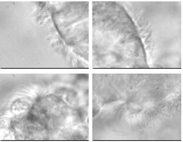
for our application, the straight linescan technique needs a straight border of cells, something not always possible with harvested cells. In the field of view, multiple cell groups are often visible, and cilia on a given cell can beat at different frequencies. As a result, many frequencies can be measured in a single field of view. Such frequencies provide information on cilia synchronization, and ultimately on the status of the cells under scrutiny. We seek to segment the field of view into regions that are consistent from the point of view of the beating pattern. Nasal brushing produces significant amounts of cells with beating cilia. The diversity in sequence appearances can be appreciated on Fig. 2.7. Brushings were all recorded under a microscope minutes after the biopsy, at 358 frames per second with a high speed camera. The spatial resolution is 0.13µm, and the resolution is 256×192 pixels. The sequence was recorded on the border of the groups.
2.2.2
Cilia beating characterization and diagnosis
Cilia beating characterization remains a significant field of study. The difficulty is to analyze not only a single cilium but a group of cilia to evaluate the efficiency of beating. Indeed, a cilium can beat at normal frequency, but if the beating is
16 2.2. Context and state of the art
Figure 2.7: Four examples of ciliated cells, showing the large variability in our samples.
irregular or not synchronized with its neighbours, the clearance can be ineffective. Practitioners have to pair the measurements [27] to evaluate the characterization, which is difficult. Some attempts have been made to help the diagnosis of primary diskinesis patient such as in [28]. In that article, the procedure classifies the sequences in two categories (ill or healthy) with a machine learning procedure based on optical flow. In this study, authors show a significant distinction between classes but do not attempt to measure parameters interpretable by clinician, which would be useful for differential diagnosis.
Work in this field is ongoing but as yet not entirely conclusive.
2.2.3
Estimating cilia behaviour in vivo
The evaluation of mucociliary clearance in vivo has always been a challenge. The most reliable measurement consists of a saccharin protocol described by Andersen
et al. in 1974. This method consists of applying particles of saccharin on the nasal
mucous membrane and to measure the time spent before the patient detect a sweet taste. This method depends of the sensitivity of patients and is not sufficient to diagnose diseases. The only way to evaluate reliably the mucociliary clearance for diagnosis is the ex-vivo methods described above. They remain invasive for patients
2. Ciliated cells analysis 17
because of the need for a biopsy, and the analysis is tedious to carry out, and so results can be slow to obtain. Moreover, cells can be injured during the biopsy leading to unreliable results. Finally, there remain questions about the behavior of cells in-situ and ex-situ.
For all these reasons, we sought to develop a procedure for observing and analysing cilia in vivo. This is extremely challenging because cilia are small (10µm in length, 0.1µm in diameter) and beat at relatively high frequency, from 0 to 30Hz. The results of the experiments related to these developments are reported in chapter 9.
In this chapter we presented the motivation for ciliated cells analysis and the context of the study. We now describe the eco-toxicity, begining with the reasons for using fish embryos.
3
Fish embryos and eco-toxicity
Fish embryo models are used increasingly for human disease modeling, chemical toxicology screening, drug discovery and environmental toxicology studies. These studies are devoted to the analysis of a wide spectrum of physiological parameters, such as mortality ratio or heart rate frequency.
Contents
3.1 Context . . . . 20 3.2 The fish embryo model . . . . 20 3.3 Image processing and fish studies . . . . 21
20 3.1. Context
3.1
Context
In recent years, it has become mandatory for the cosmetics industry to warrant the harmlessness of the products and compositions that they manufacture [29]. This includes the by-products and refuse of the manufacturing process as well as the degradation results of the products once released into the environment [30]. However, the cosmetics industry may no longer use animals for any study [31]. Fortunately, some living organisms are still permitted for toxicology assays. Among those, some varieties of fish embryos, particularly those that are easily available and do not require difficult husbandry techniques, are particularly suitable. Fish embryo are defined here as the stage of development following spawning but such that the yolk sac is still attached. At this stage, these organisms feed autonomously and passively from yolk nutrients and are not considered animals. Their size is small (a few mm in length) but do not require high-power microscopes or sophisticated image acquisition devices: a simple camera with a macro lens is enough. They are transparent, and so analyses can be carried out without using invasive techniques. Their circulatory system, in particular, including the heart and major blood vessels, is easily visible. Since they live in water they are ideal for studying waterways pollution [32]. These organisms also belong to the vertebrata subphylum, like humans. For all these reasons, they have been used as model organisms in toxicology studies for quite some time [33]. In the cosmetics industry, large numbers of compounds and formulation need to be tested for health-related effects. L’Oréal for example, use a range of five concentrations per chemical compound. For replication this represents one 24-well plate per concentration plus one plate with no compound present for comparison, for a total amount of 6 plate i.e. 144 wells per test. Because many chemical compounds need to be tested (several tens of thousands in the context of the cosmetics industry alone), this represents several millions of measurements. Manual or semi-automated procedures are no longer sufficient for this task [34].
3.2
The fish embryo model
The fish embryo model has become a classical model in research, and so in toxicology assays. The two most popular organisms used as models are Zebrafish and Medaka. Zebrafish (Danio rerio) is a small fish member of genus Danio, and Medaka (Oryzia
latipes) is a small fish member of genus Oryzias.
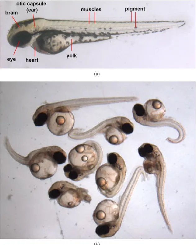
Both have fast development and are cheap husbandry. Moreover, both are tranparent (see Fig. 3.1(a)) during the embryo phase, ensuring that their organs are visible and so readily analyzable. They are important model organisms for in vivo studies of vertebrates in biology, toxicology, health, and fundamental research [35,36,37,38]. They are also used in new research fields such as nano-toxicity [39] (see Fig 3.1(b)). Their genetic material is well studied and bears some resemblance to that of humans: humans and zebrafish share 85% of their genome [40], making it a good model for toxicity studies. Moreover, their genome can be modified to express susceptibility to some diseases, or to imbue some of their organs with auto-fluorescence. We recall that while they are still embryos, they are not considered as lab animals and so can
3. Fish embryos and eco-toxicity 21
be used for studies without special authorizations.
Zebrafish is somewhat smaller than Medaka and is more pigmented. In our studies transparency is essential, so they are not used for the same studies. We mainly studied the Medakas embryos. In our study, embryo were procured from Amagen (UMS 3504 CNRS / UMS 1364 INRA). They are placed as eggs in a neutral environment with Methylene blue to detect dead eggs, and incubated for 9 days at a temperature of 28◦C. Embryos do not feed, so no nutrients are supplied. They were anesthetized with tricaine (0.1 g/L) immediately before study.
The protocol for fish analysis is always the same regardless the species or the technique. This protocol is illustrated in Fig. 3.2.
3.3
Image processing and fish studies
Image processing has been widely used in conjunction with fish studies, for instance for sizing [42], aging analysis [43], species recognition [44], automated counting [45], behaviour assessment [46,47], and more recently for supervising micro-injections in fish embryo [48]. Indeed, fully automated image analysis can offer an interesting alternative to manual procedures, capable of rising to the challenge of offering fast and reliable vital signs assessments in fish embryos [49, 50].
In [41], Mikut and al. present a survey on the existing automated processing for fish embryo image analysis, and here for Zebrafish.
One of the most common vital sign is the pattern of a beating heart, and one of the strongest effect of toxic molecules is to induce death. It is hence meaningful to study the presence of a beating heart to evaluate the lethality of compounds. In our study, we focused on the analyze of cardiac characteristics of Medaka embryos. To comply with industrial demands, the procedures have to be entirely automated. Speed and reproducibility favor reducing the action of humans during the entire protocol (see workflow on Fig. 3.2). Some tools already exists for automating all the non-imaging related protocol steps, such as the Hamilton robots1 that cleanse and
handle fish embryos and various molecules in the plate wells without any human intervention. For the acquisitions, the plates have to be removed from the apparatus, and brought to the acquisition system. This system can be manual (microscopy for example) or automated (the VAST system for Zebrafish 2 can take time-lapse
images of a Zebrafish in a capillary glass vessel. Image analysis system vendors such as FEI 3 with Visilog, or Definiens can propose automated plaforms for taking
images and videos of twell plates without requiring a microscope or a fast camera). These automated tools have some limitations. The VAST system is currently only available for Zebrafish, in which they are a very tight fit. Consequently they are not suitable for Medaka or Zebrafish with serious malformations. Visilog tool is not particularly well suited to analyze sequences, but is capable of detailed 2D studies, for instance including embryo malformations.
1 http://www.hamiltoncompany.com 2 http://www.unionbio.com/vast/ 3 https://www.fei.com
22 3.3. Image processing and fish studies
(a)
(b)
Figure 3.1: Anatomy of a Zebrafish larva, fromhttp://www.devbio.biology.gatech.
edu/?page_id=399 and Medakas’ malformation as a result of being exposed to nano
3. Fish embryos and eco-toxicity 23
Figure 3.2: Workflow for fish analysis procedure (modified from [41]).
Some automated software packages for the analysis of various embryo characteristics do exist. A quantification of Zebrafish behaviour from low temporal resolution video sequences was proposed in [47]. A screening method to estimate heart frequency exists in the form of a patent [51], but is sensitive to noise and requires a high spatial resolution. The photocardiography method [52] is promising but requires specific tools. ViewPoint developed an automatic tool to measure heartbeat frequencies in Zebrafish via bloodflow analysis4, but their method is not open-source and twe
have not found clear documentation describing their methodology.
One challenge is to adapt existing tools to the available platform and industrial constraints. The methods has to be reliable, easy to use, robust and fast, and finally it has to be adapted to the demands of industrial applications.
We note that some analyses can be simplified by using stainings and other markers. For instance using methylene blue, dead eggs and embryos can be easy to detect as they become dark as the pigment concentrates in the dead organisms.
In most cases, however, a readily available staining does not exist and so a specific image analysis procedure must be developed.
In this chapter, we have presented our second field of application. We now present the image analysis tools we developed, with a first chapter summarizing the methodologies we proposed.
4
Part II
Technical contributions
4
Methodology essentials
This chapter sumarizes in less technical terms all the methodologies presented in the following three chapters. the objective of this chapter is to communicate the essential developments that we propose while eschewing technical jargon, for a broader audience.
Contents
4.1 Tools . . . . 28 4.1.1 Sensor pattern removal . . . 28 4.1.2 Sequence stabilization . . . 29 4.2 Simple motion analysis . . . . 30 4.2.1 Motion highlighting . . . 30 4.2.2 Motion segmentation by temporal gradient . . . 30 4.2.3 Motion segmentation by temporal variance . . . 31 4.2.4 Spurious motion elimination . . . 31 4.2.5 Frequency estimation . . . 31 4.3 Complex motion analysis . . . . 32 4.3.1 Feature-based region segmentation . . . 32 4.3.2 Curvescan . . . 32
28 4.1. Tools
4.1
Tools
Many image processing, image analysis and computer vision techniques were used in this thesis. We summarize these in technical details in chapter 5. That chapter also contains two applications for removing artifacts, which we present here in a simpler context. These two applications are the “Sensor pattern removal" and the “Image stabilization procedure". We developed these applications because of our experimental constraints that induce strong artifacts on our sequences. The two main artifacts we faced were:
• Sensor pattern. Most of our image data were acquired under a microscope using high speed camera. Due to constraints in high-speed sensor design, the captured sequences look like they are taken behind a non-moving grid. This grid is the sensor pattern relative to the camera itself and must be removed before any further the analysis as it affects the quality of the sequences. • Undesirable motion. As we are studying motion, undesirable motion
artifacts can induce incorrect results. Because we are working on living organisms that have to be kept in a liquid medium even during the analysis, the probability of observing undesired motion such as vibrations, sliding etc. increases and these have to be corrected for.
These two points have to be handled in a precise order: first the sensor pattern removal and then the motion correction. The reason of this order is that if we started the other way, the texture of the camera would no longer be fixed, and would induce a new type of artifact that would be more difficult to remove.
4.1.1
Sensor pattern removal
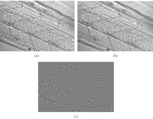
The sensor pattern is a fixed, texture-like grid. When we do not remove this texture, watching the sequence is like through a noisy grid. More importantly, this fixed grid artifact perturbs motion detection and induces further artifacts.
To remove it, we have first to identify it. By computing the average image of the sequence, only the immobile parts of the sequence including the grid remain. Indeed, since the time-wise average of a non-moving element is this element itself. But the average image also provides other meaningful information on the sequence, and not just the grid, so we have to separate the grid from the rest of the average image (for example something moving slowly). Because the grid is composed of fairly isolated pixels of different varying grey-level intensities (like a lattice), we can blur the average image with a small Gaussian filter: this erases only the small components including the grid, and slightly blur the other components.
The result is an average image with the grid and one without (see 5.14). The grid is identified by subtracting these 2 images. We can now remove the identified grid from all frames of the sequence without affecting the quality of the sequence.
4. Methodology essentials 29
4.1.2
Sequence stabilization
We need to stabilize the object of study. For this we are going to perform a so-called “registration" between the objects on the frames. Registration allows to superimpose objects between frames. Using a registration method permits to stabilize the sequence, as the object of study, once registered, appears in the same fixed position in all the images of the sequence.
We use a registration method based on “key points". A key point is a point located with high precision on the image, associated with a set of “descriptors". The descriptors describe the point itself and its environment. A keypoint is a point whose descriptors are sufficiently specific to be distinguished from other nearby points.
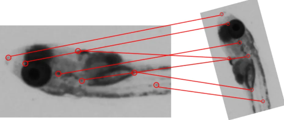
Registration uses a reference frame and a moving frame. The idea is to consider a point in the reference frame and to find its corresponding point in the moving frame. A set of 2 corresponding points forms a pair. With a large enough set of pair, we are able to find the transform between the coordinates of the points in the reference frame and in the moving one. The figure below illustrates this.
We have X = R × X0 + T where R is the rotation matrix and T the translation (more detailed equations are given in the methodology paragraph). It means that to superimpose the points between the two frames, we need to apply a transform on a set of point. In our case, we consider 3 families of transforms: identity (i.e. no transformation at all), translation only and translation + rotation. These are called “rigid" transform because they do not change the scale or the shape of the objects. We selected the best transform by comparing the differences between each result with the reference frame. We consider these three cases in succession because if we look for a complex transform we always find parameters for it, but sometimes the parameters are not significant.
We transformed our sequence using this method in order to obtain a stabilized sequence.
30 4.2. Simple motion analysis
4.2
Simple motion analysis
We present here tools that we used for the analysis of simple motion such as heart frequency estimation. These tools are independent of each other. They can be used alone or in combination with others, depending on the aim of the study. We recommend to apply these procedures at least after image stabilization procedure if the sequence shows undesirable motion, to ensure that the moving parts are components of interest.
4.2.1
Motion highlighting
This procedure erases all the fixed elements of a sequence, so that only the moving part are visible. Because we are working on motion analysis, it is useful to enhance the sequences by highlighting the moving components of this sequence. This procedure is intended to be used in a sequence where there is no longer any motion artifact present, so after sequence stabilisation is performed.
We used again the time-wise averaging method: the average of a stabilized sequence yields an image of the non moving parts of this sequence. We do not need to blur this image, as it is non-moving. We just subtract this average from all the frames of the sequence, yielding a sequence consisting only of the moving parts.
4.2.2
Motion segmentation by temporal gradient
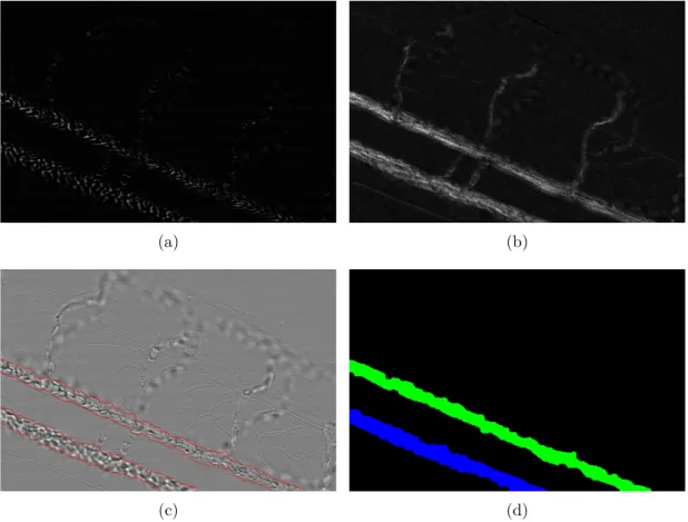
We present here a simple segmentation (i.e. separation) between fixed and moving parts in a sequence. It is possible to visualize the motion between two frames when computing the difference between two frames. This allows us to detect what changes between the two frames (see for example fig. 11.4(a)). The asymmetric temporal gradient is a sequence of the difference between each frame and the one immediately after it. When we sum this temporal gradient, this shows all the area where motion occurred during the entire sequence, in a single image (see fig. 11.4(b)). It is not however of interest to us to consider the motion over a whole sequence. This could be difficult to interpret since slow motion components would begin to play a part. So we do integrate (we sum) the sequence only over a few frames. In these integrated images, the intensity represents the amount of change. The highest intensities refer to the largest motion. We filter the slow motion pixels with a threshold: all the pixels under the threshold value are set to 0. This value is determined with an adaptive thresholding method named “Otsu’s criterion". It automatically adapts this value to the content of the image. We then connect the pixels of this image with morphological tools (see Chap. 5.2.1 for the definitions and explanations of erosion and dilation). We obtain an image of the motion areas where each pixel belonging to an area have the same value (see fig. 11.4(d)).
4. Methodology essentials 31
4.2.3
Motion segmentation by temporal variance
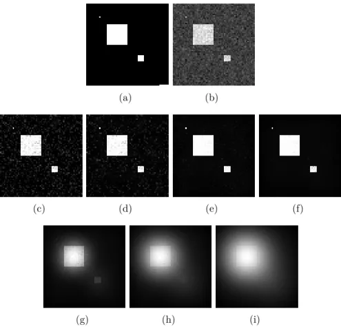
We also developed a method to segment motion areas with a more general criterion called the temporal variance. For this we calculate the same temporal gradient as previously, but we do not perform a simple sum. Instead we compute a time-wise variance at each pixel location, i.e. we consider the set of values that a particular pixel takes over time. This hilights the areas where motion is present. This yields an image of where motion is present. To blend irrelevant variations, we perform a spatial Gaussian blur, which smooths the resulting image. Each resulting smooth blob corresponds to an area of motion. We then segmented each area with “Watershed procedure", described in chapter 5. In essential terms, the watershed procedure finds an optimal contour between sets of “markers", which are areas in the image that are characteristic of the inside of the objects of interest (inner markers) and of the outside of objects (outer markers). The markers of the watershed were obtained using morphological tools, the inner markers are the highest values of each blob, and the outer marker is the area where no motion is detected. We then obtain a segmentation in which each region is related to a local maximum motion intensity.
4.2.4
Spurious motion elimination
Cyclic motion can be distinguished from other kinds of motions by their own characteristics, and can be of interest (the heartbeat for example is a cyclic motion). Cyclic motion is a motion that has a repeated pattern over time. We developed a tool that distinguishes cyclic motion from other kinds of motion. If we split the sequence into sub-sequences long enough to contain one cycle, we will notice the same (or nearly the same) motion in each sequence, whereas spurious motion will not appear on all sub-sequence. By computing the variance of each sub-sequence, we highlight the main motion in the sub-sequences, which will always be present in the case of cyclic motion. The median of all sub-sequences yields the motion that is present on the majority of the sub-sequences, especially the cyclic motion.
4.2.5
Frequency estimation
The estimation of frequency is a parameter that is of interest for clinicians interested in diseases involving cilia, or for eco-toxicity studies. We developed several automated or semi-automated methods to estimate frequencies.
Semi-automatic grey-level intensity based frequency estimation
A semi-automatic way for the estimation of frequency is to measure the variations of grey-level intensities, for instance by computing the average pixels intensities in a window. Frequencies can be estimated by Fourier analysis on this signal.
Optical flow
Optical flow is the apparent motion between frames. Computing the optical flow means provides a local translation vector field between these frames. In our work, we developed an automatic optical flow-based method to evaluate frequency in
32 4.3. Complex motion analysis
areas of interest. When we study the intensity of this vector field, which we term "displacement" in the following, we can observe variations: they correspond to speed variations, which can yield frequency information. For each motion region detected, we hence obtain a displacement vector which is the median of all the displacement vectors belonging to that region. The analysis of the variation of the magnitude with a Fourier transform yields the frequency in the region.
4.3
Complex motion analysis
Some parameters may be more difficult to analyze than others. Because we do not always know in advance the characteristics of the motion under study, we developed tools that are suitable for complex motion analysis.
4.3.1
Feature-based region segmentation
A powerful approach is to take into account beating patterns when segmenting areas of motion. Each region should correspond to a single motion pattern, and so moving elements in this region should be moving in a similar way. Because we are mostly interested in beating patterns, and these patterns are periodic, it makes sense to use Fourier analysis. Using Fourier analysis, we compute the power spectrogram of the luminosity at various scales in a moving square window. Each spectrogram forms a “signature", or a vector of features that can be compared with the feature vector of the neighboring regions. We use a clustering method to compare vectors and separate groups, each with sufficient beating pattern similarity. This allows us to identify markers, which are groups of pixel with the highest similarity-score and so beat in the same way. We then attribute the remaining pixels according to their similarity and proximity with the seeds to an area. For each pixel, our procedure yields a score of similarity with each seed, from which we derive region identifications. This procedure ensures that in each region, the behavior of its moving elements is coherent.
4.3.2
Curvescan
Assuming we achieve a reasonable segmentation of areas of motion, we are interested in analyzing the trajectories of the objects belonging to these regions. It is useful to visualize the path followed by the objects of interest in the sequence, in particular the trajectories of cilia. An idea is to outline the pattern they draw while beating. We can imagine that cilia have a pen at their extremity, and they are made to draw their path over time, like on seismographs. The curvescan is derived from this idea. To capture these trajectories, we use the contours of our segmentation. The segmentation surrounds cilia. The contour of this segmentation are typically located near the cilia extremities. By taking the first frame, we obtain this contour, and we "unroll" it: we obtain the position of each extremity of cilia in the first image. We paste it in a new image. Then we do the same thing in the second image, the third etc and we paste the new unrolled contour below the previous one like in
4. Methodology essentials 33
Figure 4.1: Distance map simplification: the red line is the line labeled 1 because it is necessary to only cross 1 pixel to reach the background, the yellow is labeled 2 because crossing two pixels is now necessary, etc.
the linescan: we obtain a follow-up of the position of cilia. The difference between linescan and curvescan is the shape of the studied pixels. To obtain our curves, we computed a "distance map" to our segmentation: it attributes to each pixel of the segmentation the value of its minimal distance to the background (see Fig. 4.1). We can then study all the curves present in our segmentation by doing this procedure on each line of the distance map.
In the next Chapter, we provide all the technical details for the tools that we have developed during the course of our research. Readers who are not interested in a high level of technical details regarding our image analysis contribution may directly skip to part III, describing the applications.
5
Tools for motion analysis
This chapter gives a presentation of the basic image processing tools we used in our study.
All the data we analyzed were acquired on devices such as bright field, fluores-cence or stereo-microscopes, and were recorded with digital cameras. the organisms we studied, whether fish embryo or ex-vivo biopsy samples, were imaged in a fluid. The protocols we used are fraught with artifacts that need to be removed before motion analysis in the videos. These artifacts typically consist of noise or undesirable motion.