HAL Id: hal-01898905
https://hal.archives-ouvertes.fr/hal-01898905
Submitted on 19 Oct 2018
HAL is a multi-disciplinary open access
archive for the deposit and dissemination of
sci-entific research documents, whether they are
pub-lished or not. The documents may come from
teaching and research institutions in France or
abroad, or from public or private research centers.
L’archive ouverte pluridisciplinaire HAL, est
destinée au dépôt et à la diffusion de documents
scientifiques de niveau recherche, publiés ou non,
émanant des établissements d’enseignement et de
recherche français ou étrangers, des laboratoires
publics ou privés.
Time warp invariant dictionary learning for time series
clustering: application to music data stream analysis
Saeed Yazdi, Ahlame Douzal-Chouakria, Patrick Gallinari, Manuel
Moussallam
To cite this version:
Saeed Yazdi, Ahlame Douzal-Chouakria, Patrick Gallinari, Manuel Moussallam.
Time warp
in-variant dictionary learning for time series clustering: application to music data stream analysis.
ECML/PKDD, 2018, Sep 2018, Dublin, Ireland. �hal-01898905�
Time warp invariant dictionary learning for time
series clustering: application to music data
stream analysis
Saeed Varasteh Yazdi1, Ahlame Douzal-Chouakria1, Patrick Gallinari2, and Manuel Moussallam3
1
Univ. Grenoble Alpes, CNRS, Grenoble INP, LIG, Grenoble, France [email protected], [email protected],
2
Universit´e Pierre et Marie Curie, Paris, France [email protected]
3
Deezer, Paris, France [email protected]
Abstract. This work proposes a time warp invariant sparse coding and dictionary learning framework for time series clustering, where both in-put samples and atoms define time series of different lengths that involve variable delays. For that, first an l0 sparse coding problem is formalised
and a time warp invariant orthogonal matching pursuit based on a new cosine maximisation time warp operator is proposed. A dictionary learn-ing under time warp is then formalised and a gradient descent solution is developed. Lastly, a time series clustering based on the time warp sparse coding and dictionary learning is presented. The proposed approach is evaluated and compared to major alternative methods on several public datasets, with an application to deezer music data stream clustering. Keywords: Time series clustering, dictionary learning, sparse coding
1
Introduction
Sparse coding and dictionary learning become popular methods in machine learn-ing and pattern recognition for a variety of tasks as feature extraction, recon-struction and classification. The aim of sparse coding methods is to represent input samples as a linear combination of few basis functions called atoms com-posing a given dictionary. Sparse coding problem is formalised basically as an optimisation problem that minimises the error of the reconstruction under l0 or l1 sparsity constraints. The l0 constraint leads to a non convex and NP-hard problem, that can be solved efficiently by pursuit methods such as orthogonal matching pursuit omp[15]. Relaxing the sparsity constraint from l0 to l1 norm yields a convex sparse coding problem, also known as lasso problem [14]. The dictionary for the sparse representation can be selected among pre-specified fam-ily of basis functions (e.g. gabor) or be learned from the training data to sparse represent the input data. A two-step strategy is commonly used: 1) keep the
dictionary fixed and find a sparse representation by using a sparse approxima-tion, 2) keep the representation fixed and update the dictionary, either all the atoms at once[6]or one atom at a time[2]. In the context of classification, the dictionary is generally learned from the labeled training dataset and the sparse codes of the testing samples are used for their classification[9,10,17]. In cluster-ing settcluster-ing, we distcluster-inguish two principal sparse codcluster-ing and dictionary learncluster-ing approaches. The first category of approaches assumes the data structured into a union of subspaces[3,5,16,18]where each sample may be represented as a linear combination of some input samples that ideally belong to the same subspace. Several of these approaches are related to sparse subspace clustering where sam-ples are first sparse coded based on the input set as a dictionary [5,18], then a spectral clustering[11]of the sparse codes is used to cluster the data. The num-ber of subspaces as well as their dimension may be fixed beforehand or induced from the affinity graph. In the second category of approaches, a sparse coding and dictionary learning framework is proposed to simultaneously learn a set of dictionaries, one for each cluster, to sparse represent and cluster the data[12].
For temporal data analysis, sparse coding and dictionary learning are espe-cially effective to extract class specific latent temporal features, reveal salient primitives and sparsely represent complex temporal features. However, what makes temporal data particularly challenging is that salient events may arise with varying delays, be related to a part of observations that may appear at different time stamps. This work addresses the problem of time series cluster-ing under sparse codcluster-ing and dictionary learncluster-ing framework, where both input samples and atoms define time series that may involve varying delays and be of different lengths. For that, in the first part, an l0 sparse coding problem is formalised and a time warp invariant orthogonal matching pursuit based on a new cosine maximisation time warp operator is proposed. Subsequently, the dic-tionary learning under time warp is formalised and a gradient descent solution is developed. In the second part, a time series clustering approach based on the time warp invariant sparse coding and dictionary learning is proposed. The main contributions of the paper are:
1. We propose a time series clustering approach under sparse coding and dic-tionary learning setting.
2. We propose a tractable solution for time warp invariant orthogonal matching pursuit based on a new cosine maximisation time warp operator.
3. We provide a sparse representation of the clustered time series and learn, for each cluster, a sub-dictionary composed of the most discriminative prim-itives.
4. We conduct experiments on several public and real datasets to compare the proposed approach to the major alternative approaches, with an application to deezer music data stream clustering.
The reminder of the paper is organised as follows. Section2formalises the time series clustering problem under sparse coding and dictionary learning setting. Section 3 proposes a solution for sparse coding and dictionary learning under time warp, then presents the time series clustering method. Finally, Section 4
presents the experiments and discusses the results obtained.
2
Problem statement
This Section formalises the time warp invariant sparse coding and dictionary learning for time series clustering. In the following, bold lower case letters are used for vectors and upper case letters for matrices. Let X = {xi}Ni=1 be a set of N input time series xi = (xi1, ..., xiqi)
t
∈ Rqi of length q
i. We formalise the problem of time series clustering under the sparse coding and dictionary learning setting as the estimation of: a) the partition C = {Cl}Kl=1 of X into K clusters and b) the K sub-dictionaries {Dl}Kl=1, to minimise the inertia goodness criterion (i.e., the error of reconstruction) as:
min C,D K X l=1 X xi∈Cl E(xi, Dl) (1) where Dl = {dlj} Kl
j=1 the sub-dictionary of Cl is composed of Kl time series atoms dlj ∈ Rpj. Note that, both input samples x
i and atoms dlj define time series of different lengths that may involve varying delays. E(xi, Dl) the error of reconstruction, under time warp, of xibased on the sub dictionary Dl= {dlj}
Kl j=1 is formalised as: E(xi, Dl) = min αi kxi− Fi(Dl)αlik 2 2 s.t.kα l ik0≤ τ. (2) where Fi(Dl) = [fi(dl1), ..., fi(dlKl)] ∈ R qi×Kl is the transformation of D l to a new dictionary composed of warped atoms fi(dlj) ∈ Rqialigned to xito resorb the involved delays w.r.t xi. αli= (α
l 1i, ..., α
l Kli)
tis the sparse codes of x iunder Dland τ the sparsity factor under the l0 norm.
3
Proposed solution
To resolve the clustering problem defined in Eq.1, we use a two steps iterative refinement process, as in standard kmeans clustering. In the cluster assignment step, Dl’s are assumed fixed and the problem remains to resolve the sparse coding based on the warped dictionary Fi(Dl) defined in Eq.2. The cluster assignment is then obtained by assigning each xi to the cluster Cl whose sub dictionary Dl minimises the reconstruction error. In the dictionary update step, the learned sparse codes and the clusters Cl are that time fixed and the problem in Eq. 1 defines a dictionary learning problem to minimise the clustering inertia criterion and represent sparsely samples within clusters. For the cluster assignment, we propose in Section3.1, a time warp invariant orthogonal matching pursuit based on a new cosine maximisation time warp operator. In Section 3.2, a gradient descent solution for dictionary learning under time warp is developed, then the clustering algorithm for time series under sparse coding and dictionary learning setting is given in Section3.3.
3.1 Time warp invariant sparse coding
For the sparse coding under time warp problem given in Eq.2, we define Fi(Dl) as a linear transformation of Dlbased on the warping function fi(dlj) = ∆lijd
l j, where the projector ∆l
ij ∈ {0, 1}qi×pj specifies the temporal alignment that re-sorbs the delays between xiand dlj. The problem given in Eq.2is then formalised as: min αi, ∆li kxi− Kl X j=1 ∆lijd l j αjil k22 (3) s.t. kαlik0≤ τ, ∆lij ∈ {0, 1} qi×pj, ∆l ij1pj = 1qi. with ∆li= {∆lij}Kl
j=1. The last constraint is a row normalisation of the estimated ∆l
ij to ensure for xi equally weighted time stamps. To resolve this problem, we propose an extended variant of omp that can be mainly summarised in the following steps:
1. For each dlj, estimate ∆l
ij by dynamic programming to maximise the cosine between xi and dlj.
2. Use the projector ∆l
ij to align d l j to xi.
3. Estimate the sparse codes αli based on the aligned atoms. For that and to estimate ∆l
i, we propose a new operator costw to estimate the cosine between two time series under time warp. To the best of our knowledge, it is the first time that the cosine operator is generalised to time series under time warp. Then, we present a time warp invariant omp (twi-omp), that extends the standard omp approach to sparse code time series under non linear time warping transformations.
Cosine maximisation time warp (costw): The problem of estimating the cosine between two time series comes to find an alignment between two time series that maximises their cosine. Let x = (x1, ..., xqx), y = (y1, ..., yqy) be two
time series of length qx and qy. An alignment π of length |π| = m between x and y is defined as the set of m increasing couples:
π = ((π1(1), π2(1)), (π1(2), π2(2)), ..., (π1(m), π2(m)))
where the applications π1and π2defined from {1, ..., m} to {1, .., qx} and {1, .., qy} respectively obey the following boundary and monotonicity conditions:
1 = π1(1) ≤ π1(2) ≤ ... ≤ π1(m) = qx 1 = π2(1) ≤ π2(2) ≤ ... ≤ π2(m) = qy and ∀ l ∈ {1, ..., m},
π1(l + 1) ≤ π1(l) + 1 , π2(l + 1) ≤ π2(l) + 1, (π1(l + 1) − π1(l)) + (π2(l + 1) − π2(l)) ≥ 1
Algorithm 1M axT riplet(u, v, z) Input: u, v and z.
1: if f (u) ≥ f (v) and f (u) ≥ f (z) then 2: return u;
3: else if f (v) ≥ f (u) and f (v) ≥ f (z) then 4: return v;
5: else 6: return z; 7: end if
Intuitively, an alignment π between x and y describes a way to associate each element of x to one or more elements of y and vice-versa. Such an alignment can be conveniently represented by a path in the qx× qy grid, where the above monotonicity conditions ensure that the path is neither going back nor jumping. We will denote A as the set of all alignments between two time series. The cosine maximisation time warp can be formalised as:
costw(x, y) = s(π∗) (4) π∗= arg max π∈A s(π) s(π) = P|π|
i=1xπ1(i)yπ2(i)
q P|π| i=1x 2 π1(i) q P|π| i=1y 2 π2(i)
where s(π) is the cost function of the alignment π. The solution for costw is obtained by dynamic programming thanks to the recurrence relation detailed here after.
Let xqx−1 = (x1, ..., xqx−1), yqy−1 = (y1, ..., yqy−1) be two sub-time series
composed of the qx− 1 and qy− 1 first elements of x and y, respectively. In the case of aligned time series, that do not include delays and with the same length (i.e., qx= qy) the following incremental property of the standard cosine can be established: cos(xqx−1, yqy−1) = f (< xqx−1, yqy−1>, kxqx−1k 2 , kyqy−1k 2 ) cos(x, y) = f ((< xqx−1, yqy−1>, kxqx−1k 2 , kyqy−1k 2 ) ⊕ (xqx, yqy)) (5)
where f is a real function defined as f (a, b, c) = √a
b√c with (b, c ∈ R ∗
+) and ⊕ is an operator that associates to a triplet (a, b, c) and a couple (u, v) a new triplet as:
(a, b, c) ⊕ (u, v) = (a + uv, b + u2, c + v2)
For time series including delays and based on the incremental property given in Eq. 5, let us introduce the computation and recurrence relation that allows to estimate the alignment π∗ that maximises costw(x, y) in Eq.4.
Computation and recurrence relation: Let us define M ∈ Rqx×qy the
Algorithm 2twi-omp(x, D, τ ) Input: x, D = {dj}Kj=1, τ
Output: α, ∆ 1: r = x, Ω = {φ} 2: while |Ω| ≤ τ do
3: Select the atom dj(j /∈ Ω) that maximizes |costw(r, dj)|
4: Update the set of selected atoms Ω = Ω ∪ {j} and SΩ= [∆jdj]j∈Ω
5: Update the coefficients: αΩ= (STΩSΩ)−1(SΩTx)
6: Estimate the residual: r = x − SΩαΩ
7: end while
incremental property established in Eq. 5, computing recursively for (i, j) ∈ {1, ..., qx} × {1, ..., qy} the terms Mi,j as:
∀ i ≥ 2, j = 1 Mi,1= (ai−1,1, bi−1,1, ci−1,1) ⊕ (xi, y1) ∀ j ≥ 2, i = 1 M1,j = (a1,j−1, b1,j−1, c1,j−1) ⊕ (x1, yj) and ∀ i ≥ 2, j ≥ 2
Mi,j = M axT riplet
(ai,j−1, bi,j−1, ci,j−1) ⊕ (xi, yj) (ai−1,j, bi−1,j, ci−1,j) ⊕ (xi, yj) (ai−1,j−1, bi−1,j−1, ci−1,j−1) ⊕ (xi, yj)
and M1,1 = (x1y1, x21, y12), we obtain costw(x, y) = f (Mqx,qy) with a quadratic
complexity of O(qxqy). The two first equations give the first row and column updates, the third equation gives the recurrence formula that ensures the cosine maximisation at each Mi,j cell and M axT riplet function (Algorithm1) retains the triplet that maximises the cosine at Mi,j.
Time warp invariant OMP (twi-omp): Based on the defined costw, let us present the time warp invariant omp (twi-omp) to sparse code a given time series x based on a dictionary D = {dj}Kj=1under time warp conditions (Algo-rithm2). The proposed twi-omp follows the three steps given in the previous section. First, perform a costw between x and each djto estimate ∆ = {∆j}Kj=1 and find the atom dj that maximises costw(x, dj) (line 3 in Algorithm 2). Then, update the set Ω of the yet selected projected atoms and the dictionary SΩ = [∆jdj]j∈Ω of the yet selected warped atoms (line 4). The updated SΩ is then used to estimate the sparse coefficients of x (line 5-6). The process is reiterated on the residuals of x until the sparsity factor τ is reached.
3.2 Time warp invariant dictionary learning
For the dictionary learning step, the problem in Eq. 1 becomes to learn the dictionary D under time warp where, that time, the sparse codes αl
assumed fixed as: min D K X l=1 X xi∈Cl kxi− Kl X j=1 ∆lijdljαljik2 2 s.t.kd l jk2= 1. (6)
This problem is then resolved as K single dictionary learning problems to learn each sub-dictionary Dlthat minimises the inertia of the cluster Cl:
Jl= min Dl X xi∈Cl kxi− Kl X j=1 ∆lijdljαljik2 2 (7) which is equivalent to Jl= min Dl X xi∈Cl qi X t=1 (xit− Kl X j=1 αlji X (t,t0)∈π∗ ij dljt0)2 (8) s.t. kdljk2= 1
where xitis the tthtime instant of xi and π∗ij denotes the optimal alignment path between xi and dlj. To resolve the Eq. 8, we propose a gradient descend method based on the following update rule at iteration m for the atom dlj:
dl(m+1)jt0 = d l(m) jt0 − η m ∂Jl ∂dl(m)jt0 (9) dl(m+1)j = d l(m+1) j kdl(m+1)j k2 with, ∂Jl ∂dl jt0 = X xi∈Cl qi X t=1 −2αlji(xit− αljid l jt0− αlji X (t,t00)∈π∗ ij (t006=t0) dljt00 (10) −X j06=j αlj0i X (t,t00)∈π∗ ij0 dlj0t00)
where η is the learning rate. In the following section, we show how the time warp invariant omp and dictionary learning are involved for time series clustering. 3.3 Time warp invariant dictionary learning for time series
clustering
For time series clustering, the clustering criterion given in Eq. 1 is minimised by an iterative process involving, respectively, time warp invariant sparse cod-ing (twi-omp) and dictionary learncod-ing for cluster assignments and dictionary
Algorithm 3twi-dlclust(X, K, τ ) Input: X = {xi}Ni=1, K, τ .
Output: {C1, ..., CK}, {D1, ..., DK}
1: {Clustering Initialisation:}
2: Define the affinity matrix S ∈ RN ×N of general term: 3: sii0=costw(xi, xi0)
4: Apply the affinity propagation (or spectral clustering) to cluster S into 5: K clusters: C1, ..., CK
6: {Sub-dictionary initialisation:} 7: for l = 1, ..., K do
8: Initialise Dlrandomly from Cl
9: repeat
10: Sparse code each xi∈ Cl: [αli, ∆li] =twi-omp(xi, Dl, τ )
11: Update each dlj∈ Dlby using Eq.9and10.
12: until Convergence (stopping rule) 13: end for
14: repeat
15: {Cluster assignment:}
16: Sparse code each xi∈ X based on each Dl(l = 1, ..., K):
17: [αli, ∆li] =twi-omp(xi, Dl, τ )
18: Assign xito the cluster Clwhose Dlminimises E(xi, Dl):
19: Cl= {xi/ l = min l0 kxi− PKl0 l0=1∆l 0 ijd l0 j α l0 jik 2 2} 20: {Dictionaries update:} 21: for l = 1, ..., K do
22: Update each dlj∈ Dlby using Eq.9and10.
23: end for
24: until Convergence (no changes in cluster assignments)
update steps (Algorithm 3). In the initialisation step, a clustering (e.g., spec-tral clustering, affinity propagation) is performed on the costw matrix S to determine an initial partition {Cl}Kl=1of X (line 1-5). A sparse coding and a dic-tionary learning are then performed on the samples of each cluster to initialise the sub-dictionaries {Dl}Kl=1 (line 6-13). Based on the initial partition {Cl}Kl=1 and sub-dictionaries {Dl}Kl=1, the cluster assignment step consists to perform a sparse coding of each input sample based on each dictionary Dl, then to assign it the cluster whose dictionary minimises its reconstruction error (line 15-19). Subsequently, in the dictionary update step, the atoms dlj of each dictionary are updated by using the formula given in Eq.9and10(line 20-23).
4
Experimental study
In this section, we evaluate the proposed time series clustering under dictionary learning setting (twi-dlclust) on several synthetic and real datasets, including multivariate and univariate time series, that may involve varying delays and be of different or equal lengths. The proposed twi-dlclust clustering method is
compared to two major alternative approaches, the subspace sparse clustering (ssc) [5]and the Dictionary Learning with Structured Incoherence (dlsi)[12]. For ssc, two variants ssc-bp[5]and ssc-omp[18]are studied for a sparse coding under l0and l1norms, where an orthogonal matching pursuit and a basis pursuit methods are used respectively. For dlsi, both sample-based and atom-based affinity matrix initialisations proposed in[12] are studied. The Matlab codes of these methods are available online4.
4.1 Data description
We have considered in Table 1 two groups of datasets. The first group is com-posed of the top 12 datasets for which the ground truth clustering is given. The four first datasets are composed of public multivariate time series that have different lengths and involve varying delays. In particular, digits, lower, and upper datasets give the description of 2-D air-handwritten motion gesture of digits, upper and lower case letters performed on a Nintendo (R) Wii device by several writers [4]. The char-traj dataset gives the 2-dimensional handwrit-ten character trajectory performed on a Wacom tablet by the same user [1]. The ecg-mit dataset was obtained from the mit-bih Arrhythmia[7] database where the heartbeats represented by qrs complexes. The 7 remaining datasets are composed of univariate time series of the same lengths that involve signif-icant delays [8]. The last two datasets are provided by deezer 5, the online
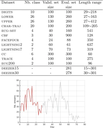
music streaming service that offers access to the music content of nearly 40 million licensed tracks. deezer data, for which we have no ground truth, give the description of streaming data of music albums, randomly selected among 105 French user streams and recorded from October 2016 to September 2017. They are composed of univariate time series that give the daily total number of streams per album from its release date to September 2017; this study con-sider only the streams of a duration ≥ 30 seconds. In particular, deezer15 and deezer30 are provided for the streams analysis over the crucial early period af-ter the album release date. They give the description of the prefix time series on the early period covering a cumulative number of 103 streams (in red in Figure 1). In addition, for the pertinence of the analysis, the prefix time series of length < 7 days are extended to 15 days in deezer15 and to 30 days in deezer30. Table1gives some characteristics of the studied datasets: the size of the clusters when the ground truth is known, the size of the validation and evaluation sets and the length of the time series that may be variable or fixed.
4.2 Validation protocol
For the top 12 datasets in Table 1, for which the ground truth partition is known, the proposed method twi-dlclust as well as the alternative clustering
4
ssc-omp: https://goo.gl/E6khsq, ssc-bp: https://goo.gl/719pvx and dlsi:
https://goo.gl/X5nZgE.
5
Table 1. Data description
Dataset Nb. class Valid. set Eval. set Length range size size digits 10 100 100 29∼218 lower 26 130 260 27∼163 upper 26 130 260 27∼412 char-traj 20 100 200 109∼205 ecg-mit 4 40 160 541 cbf 3 30 900 128 facefour 4 24 88 350 lightning2 2 60 61 637 lightning7 7 70 73 319 cc 6 300 300 60 trace 4 100 100 275 ecg200 2 100 100 96 deezer15 - - 281 15∼301 deezer30 - - 278 30∼301 0 10 20 30 40 50 60 70 80 Day 0 10 20 30 40 50 60 70 80 Nb. streams
Fig. 1. An album streaming time series, in red the prefix time series covering a cumu-lative number of 103 streams.
approaches are applied to cluster the data. For alternative methods, time series of different lengths are zero padded beforehand. The adjusted Rand index[13]is then used to evaluate the goodness of the obtained clusterings. The Rand index lies between 0 and 1, it measures the agreement between the obtained clusters and the ground truth ones. The higher the index, the better the agreement is. In particular, the maximum value ”1” of the Rand index is reached when the obtained partition and the ground truth one are identical. For deezer datasets, the ground truth being unknown, a dtw-based within-class Wr ratio6is used. The lower the within-class ratio Wr, the better the clustering is. Wr is as well used to select the optimal number of clusters. Finally, the parameters related to each studied method, indicated in Table 2, are learned by line/grid search on the validation set, the best parameters are then used to perform the clustering
6 Wr = PK l=1 P x,y∈Cldtw(x,y) P x,y∈Xdtw(x,y)
Table 2. Parameter Line/Grid values Method Line / Grid values Desc.
ssc-omp τ ∈ {1, 2, 3, 4, 5} l0 sparsity threshold
ssc-bp λ ∈ {0.001, 0.01}, lag of 0.01 l1 sparsity regularisation
dlsi λ ∈ {0.001, 0.01}, lag of 0.01 l1 sparsity regularisation
η ∈ {0, 0.1, 0.01} dictionary incoherence regularisation Kl= 5, ∀ l ∈ {1, ..., K} Sub-dictionary Dlsize
twi-dlclust sc ∈ [0, 100], lag of 10 Sakoe-Chiba band width τ ∈ {1, 2, 3, 4, 5} l0 sparsity threshold
Kl= 5, ∀ l ∈ {1, ..., K} Sub-dictionary Dlsize
on the evaluation set. The process is iterated over 10 runs and the averaged performances are reported in Tables3 and4.
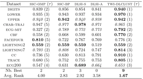
Table 3. Adjusted Rand index
Dataset ssc-omp (τ ) ssc-bp dlsi-s dlsi-a twi-dlclust (τ ) digits 0.839 (2) 0.856 0.854 0.841 0.940 (1) lower 0.935 (3) 0.943 0.937 0.934 0.970 (1) upper 0.940 (2) 0.942 0.940 0.938 0.942 (1) char-traj 0.947 (5) 0.977 0.978 0.971 0.965 (3) ecg-mit 0.327 (2) 0.789 0.772 0.773 0.792 (2) cbf 0.558 (2) 0.668 0.599 0.601 0.770 (2) facefour 0.810 (5) 0.722 0.767 0.769 0.776 (3) lightning2 0.559 (2) 0.559 0.559 0.519 0.559 (2) lightning7 0.793 (2) 0.808 0.724 0.747 0.814 (3) cc 0.736 (5) 0.630 0.813 0.791 0.910 (1) trace 0.680 (5) 0.752 0.755 0.753 0.805 (1) ecg200 0.547 (4) 0.631 0.689 0.664 0.653 (3) Nb. Best 2 2 3 0 9 Avg. Rank 4.00 2.83 2.92 3.58 1.67
4.3 Results and discussion
Table 3gives for the top 12 datasets the obtained adjusted Rand index values. The best values are indicated in bold, the non significantly different ones from the best (t-test at 5% risk) are in italic and the remaining results are signif-icantly different from the bold values. For the two l0 sparse coding methods ssc-omp and twi-dlclust, the learned sparsity coefficient τ is given between brackets. The two last rows give, over all the datasets, the number of times a method reaches the best value as well as its average ranking. From Table 3, we can see that the proposed twi-dlclust reaches the best clustering results
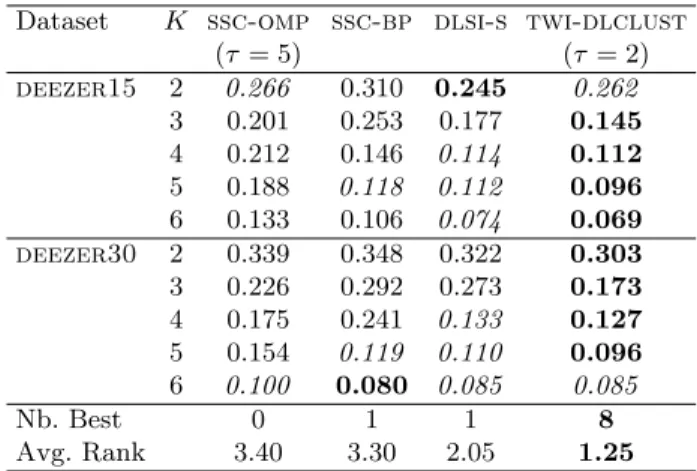
Table 4. Within-class ratio Wr per number of clusters K.
Dataset K ssc-omp ssc-bp dlsi-s twi-dlclust
(τ = 5) (τ = 2) deezer15 2 0.266 0.310 0.245 0.262 3 0.201 0.253 0.177 0.145 4 0.212 0.146 0.114 0.112 5 0.188 0.118 0.112 0.096 6 0.133 0.106 0.074 0.069 deezer30 2 0.339 0.348 0.322 0.303 3 0.226 0.292 0.273 0.173 4 0.175 0.241 0.133 0.127 5 0.154 0.119 0.110 0.096 6 0.100 0.080 0.085 0.085 Nb. Best 0 1 1 8 Avg. Rank 3.40 3.30 2.05 1.25
with 9 times (9 out of 12) as the best values, 2 times as significantly non dif-ferent from the best and obtained the lowest average ranking. The second best results are obtained by ssc-bp and dlsi-s, followed by ssc-omp. Although the l1sparse coding models (here ssc-bp and dlsi-s) are known to be more efficient than the l0models, twi-dlclust even involving an l0sparse coding leads to the best results. While twi-dlclust and dlsi-s involve smaller size sub-dictionaries (Kl= 5), ssc-omp and ssc-bp are based on larger dictionary of the size of the evaluation set (Table1). Finally, by comparing the two l0sparse coding methods ssc-omp and twi-dlclust, we can see that twi-dlclust leads for all datasets to sparser solutions with a lower or equal sparsity coefficient τ than ssc-omp. For deezer data we have performed each clustering method for several num-ber of clusters and the within-class ratio of the obtained partitions reported in Table 4. For simplicity, the dlsi approach is conducted only with dlsi-s vari-ant, dlsi-a being highly equivalent in Table3. We can see easily that, for both datasets and almost all the number of clusters, the best values are reached by twi-dlclust, followed by the l1 sparse code approaches ssc-bp and dlsi-s, then by ssc-omp. Finally, note that from both Tables 3 and 4, ssc-omp and ssc-bp lead to the lowest performances with a slightly better results for ssc-bp as using an l1norm sparse coding. These results may be partly explained by the fact that both ssc-omp and ssc-bp are purely sparse coding methods based on one global dictionary fixed beforehand, unlike dlsi and twi-dlclust that learn one sub-dictionary per cluster.
In the second study, we analyse more closely the obtained clusterings. For in-stance, based on Figure2 that displays the progression of the within-class ratio w.r.t the number of clusters, a partitioning into four clusters is performed on deezer30. Accordingly, Figure3, shows for each of the four clusters (each row), the profile of the medoids (in the first column), the closest albums to the medoid in the second column and at the third column, the atom that most contributes to sparse represent the cluster’s samples.
1 2 3 4 5 6 Nb. of clusters 0.05 0.1 0.15 0.2 0.25 0.3 0.35 Within-class ratio DEEZER15 | DSLI-S DEEZER15 | TWI-DLCLUST DEEZER30 | DSLI-S DEEZER30 | TWI-DLCLUST
Fig. 2. Number of clusters K vs. Within-class ratio Wr.
0 50 100 150 Day 0 50 100 Nb. streams
Empereur du sale | Lorenzo
0 100 200 300 Day 0 50 100 Nb. streams
Freestyle du sale | Lorenzo
0 50 100 0 0.2 0.4 0.6 0 50 100 Day 0 50 100 Nb. streams Ethologie | Dehmo 0 100 200 300 Day 0 50 100 Nb. streams
Shikantaza | Chinese Man
0 10 20 30 0 0.2 0.4 0.6 0 100 200 300 400 Day 0 50 100 150 200 Nb. streams Be Mine | Ofenbach 0 100 200 300 Day 0 100 200 300 Nb. streams
You Don't Know Me | Jax Jones
0 20 40 0 0.2 0.4 0.6 0 100 200 300 Day 0 200 400 600 800 Nb. streams ÷ (Deluxe) | Ed Sheeran 0 100 200 300 Day 0 50 100 150 Nb. streams
Le monde à l'envers | Zaho
0 10 20 30 0 0.2 0.4 0.6 C 4 C 3 C 2 C 1
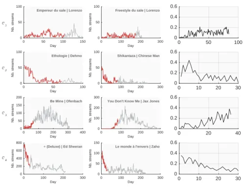
Fig. 3. Four clusters partitioning of deezer30: Medoid profile (left column), Nearest album to the medoid (middle column), the most contributing atom to the cluster (right column).
deezer data provide additional album descriptive features as ”Full” (com-posed of several tracks) or ”Single” (com(com-posed of one track), if it is a ”Deluxe” edition, namely a re-edition of the album featuring extra contents related to the album, as well as the artist popularity before and after the release. The analysis of some album characteristics brings meaningful interpretation of the extracted clusters (Figure3).
The first cluster is composed of 71% of ”Full” albums and 15% of ”Deluxe” editions. It corresponds to album releases with flat stream profiles. Such be-haviour usually occurs when the content has already been published (”Deluxe” versions) or for lesser-known artists, as assessed by the cluster medoid ”Em-pereur du Sale” album of the rapper ”Lorenzo” that released several singles a few weeks before the album release date and although not highly popular has still a steady fan base.
In the second cluster, 75% of the albums are ”Single”. The fast decrease stream profile just after the release date is not surprising for short albums (com-posed of 1-4 tracks). Indeed, a ”Full” album is generally released shortly after the ”Single” release, inducing a decrease of streams for the ”Single” few weeks after its release. The cluster medoid ”Ethologie” is produced by the rapper ”Dehmo” that has not released albums since a long period, that may explain the burst of streams for the new content just after its release.
The cluster 3 is composed of 69% of ”Full” albums mainly produced by artists that became popular after their album release. This is reflected by the stream profiles that initially evolve at low level then increase significantly several days/weeks after the album release. This is confirmed by the medoid album ”Be Mine” a single produced by ”Ofenbach” that was in fact revealed to the public with that album.
Finally, the cluster 4 comprises a majority of ”Single” albums (84%) pro-duced by very popular artists with a huge fan base and immediate success. The medoid album ”Divide” produced by ”Ed Sheeran” was one of the biggest hits of 2017. Although the stream profiles of the clusters 4 and 2 seem similar, albums of cluster 4 concern more established artists in their second/third albums while cluster 2 is more related to emerging works and first successes.
The aim of the last study is to analyse the pertinence of the learned sub-dictionaries {D1, ..., DK} for both dlsi and twi-dlclust; the dictionary for the other methods ssc-omp and ssc-bp is not learned but fixed beforehand. For that, for each method dlsi and twi-dlclust, the atoms of the learned sub-dictionaries are gathered together to built one global dictionary ∪K
l=1Dl. Let us denote DG1and DG2the global dictionaries obtained for dlsi and twi-dlclust, respectively. Subsequently, the samples in X are sparse coded, by using first an l1norm regularisation based on DG1, then a twi-omp based on DG2.
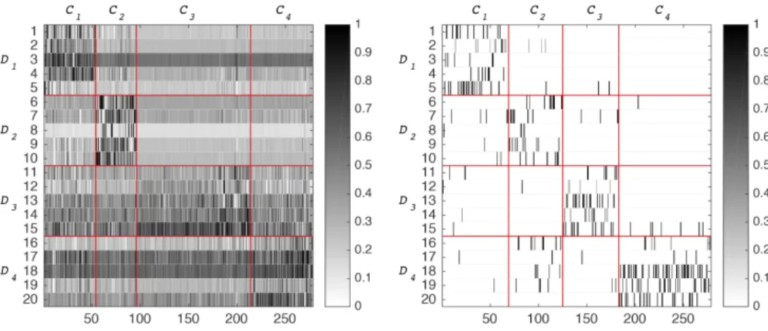
For instance, for deezer30, Figure 4 shows for the 278 albums the learned sparse codes based on DG1 (on left) and on DG2 (on right), organised for inter-pretation purpose per cluster {C1, ..., C4} and per sub-dictionary {D1, ..., D4}. It emerges from Figure4, that sparse codes based on DG2highlight clearly a block
Fig. 4. Sparse representations based on: DG1learned by dlsi (left) and DG2learned
by twi-dlclust (right).
structure that reflects the discriminative performance of the sub-dictionaries composing DG2(learned by twi-dlclust). Indeed, sparse codes show that each sub-dictionary Dlis mainly involved to reconstruct samples of Cl. On the other hand, the structure of the sparse codes based on DG1 (learned by dlsi) seems much less sparser and less discriminative. We can note, in particular, that the atoms d1
3, d315, d417and d418 define common primitives involved to reconstruct the samples of all the clusters.
5
Conclusion
This work proposes a time warp invariant sparse coding and dictionary learning for time series clustering where both input samples and atoms define time series that may have different lengths and involve varying delays. For that, first a time warp invariant orthogonal matching pursuit based on a new cosine maximisa-tion time warp operator is proposed. Then, a dicmaximisa-tionary learning approach under time warp is formalised and a gradient descent solution is developed. The pro-posed time series clustering allows to sparse represent the clustered time series and learn, for each cluster, a sub-dictionary composed of the most discrimina-tive primidiscrimina-tives. The conducted experiments show that although twi-dlclust involves an l0sparse coding approach based on a very small size sub-dictionaries, it leads to the sparser and the best clustering results, while revealing atoms with a good discriminative capacity to represent the time series of each cluster.
Acknowledgment
This work is supported by the French National Research Agency (ANR-Locust project) and Bpifrance funds in the frame of the French National PIA Program.
References
1. A. Frank, A.A.: Uci machine learning repository. http://archive.ics.uci.edu/ml/ (2010), [Online access]
2. Aharon, M., Elad, M., Bruckstein, A.: k-svd: An algorithm for designing overcom-plete dictionaries for sparse representation. Signal Processing, IEEE Transactions on 54(11), 4311–4322 (2006)
3. Bradley, P.S., Mangasarian, O.L.: K-plane clustering. Journal of Global Optimiza-tion 16(1), 23–32 (2000)
4. Chen, M., AlRegib, G., Juang, B.H.: 6dmg: A new 6d motion gesture database. In: Proceedings of the 3rd Multimedia Systems Conference. pp. 83–88. ACM (2012) 5. Elhamifar, E., Vidal, R.: Sparse subspace clustering: Algorithm, theory, and
ap-plications. IEEE transactions on pattern analysis and machine intelligence 35(11), 2765–2781 (2013)
6. Engan, K., Aase, S.O., Husoy, J.H.: Method of optimal directions for frame de-sign. In: Acoustics, Speech, and Signal Processing, 1999. Proceedings., 1999 IEEE International Conference on. vol. 5, pp. 2443–2446. IEEE (1999)
7. Goldberger, A.L., Amaral, L.A., Glass, L., Hausdorff, J.M., Ivanov, P.C., Mark, R.G., Mietus, J.E., Moody, G.B., Peng, C.K., Stanley, H.E.: Physiobank, phys-iotoolkit, and physionet. Circulation 101(23), e215–e220 (2000)
8. Keogh, E.: The ucr time series data mining archive. http://www. cs. ucr. edu/˜eamonn/ (2006), [Online access]
9. Lee, H., Battle, A., Raina, R., Ng, A.Y.: Efficient sparse coding algorithms. In: Advances in neural information processing systems. pp. 801–808 (2007)
10. Mairal, J., Bach, F., Ponce, J., Sapiro, G., Zisserman, A.: Discriminative learned dictionaries for local image analysis. In: Computer Vision and Pattern Recognition, 2008. CVPR 2008. IEEE Conference on. pp. 1–8. IEEE (2008)
11. Ng, A.Y., Jordan, M.I., Weiss, Y.: On spectral clustering: Analysis and an algo-rithm. In: Advances in neural information processing systems. pp. 849–856 (2002) 12. Ramirez, I., Sprechmann, P., Sapiro, G.: Classification and clustering via dictionary learning with structured incoherence and shared features. In: Computer Vision and Pattern Recognition (CVPR), 2010 IEEE Conference on. pp. 3501–3508. IEEE (2010)
13. Rand, W.M.: Objective criteria for the evaluation of clustering methods. Journal of the American Statistical association 66(336), 846–850 (1971)
14. Tibshirani, R.J., et al.: The lasso problem and uniqueness. Electronic Journal of Statistics 7, 1456–1490 (2013)
15. Tropp, J.A.: Greed is good: Algorithmic results for sparse approximation. Infor-mation Theory, IEEE Transactions on 50(10), 2231–2242 (2004)
16. Tseng, P.: Nearest q-flat to m points. Journal of Optimization Theory and Appli-cations 105(1), 249–252 (2000)
17. Yazdi, S.V., Douzal-Chouakria, A.: Time warp invariant ksvd: Sparse coding and dictionary learning for time series under time warp. Pattern Recognition Letters 112, 1–8 (2018),https://doi.org/10.1016/j.patrec.2018.05.017
18. You, C., Robinson, D., Vidal, R.: Scalable sparse subspace clustering by orthogonal matching pursuit. In: Proceedings of the IEEE Conference on Computer Vision and Pattern Recognition. pp. 3918–3927 (2016)