Stochastic Simulation to Improve Land-Cover Estimates Derived from Coarse Spatial Resolution Satellite Imagery
(La simulation stochastique pour améliorer les estimations de la couverture des sols à partir d’images satellitales à résolution spatiale grossière)
par
Conrad M. Bielski
Département de géographie Faculté des arts et des sciences
Thèse présentée à la Faculté des études supérieures en vue de l’obtention du grade de
Philosophiae Doctor (Ph.D.) en géographie
novembre, 2001 © Conrad M. Bielski
Université de Montréal Faculté des études supérieures
Cette thèse intitulée:
Stochastic Simulation to Improve Land-Cover Estimates Derived from Coarse Spatial Resolution Satellite Imagery
(La simulation stochastique pour améliorer les estimations de la couverture des sols à partir d’ images satellitales à résolution spatiale grossière)
présentée par: Conrad M. Bielski
a été évaluée par un jury composé des personnes suivantes:
Dr. André Roy président-rapporteur
Géographie, Université de Montréal
Dr. François Cavayas directeur de recherche Géographie, Université de Montréal
Dr. Marc D’Iorio co-directeur de recherche
Centre canadien de télédétection
Dr. Langis Gagnon membre du jury
Centre de recherche informatique de Montréal
Dr. Pierre Goovaerts examinateur externe
Civil and Environmental Engineering, University of Michigan
Dr. Jean Meunier représentent du doyen de la FES
ABSTRACT
Stochastic Simulation to Improve Land-Cover Estimates Derived from Coarse Spatial Resolution Satellite Imagery
by Conrad M. Bielski
Keywords: stochastic imaging, remote sensing, land-cover and scale change
Today’s land-cover monitoring studies at regional to global scales using optical satellite based remote sensing is confined to the use of coarse spatial resolution imagery. Due to the coarse spatial resolution, land-cover identification is poor and estimation is error prone. Some land-cover investigations apply a scaling-up approach where fine spatial resolution imagery is aggregated until the wanted mapping scale is attained. Here, the opposite approach (scaling-down) is investigated through the use of geostatistical stochastic imaging techniques. The objective of this thesis is to examine the possibility of generating finer spatial resolution multi-spectral like images based on available multi-spectral coarse spatial resolution imagery to extract land-cover information. Other ideas addressed were: a) whether stochastic imaging can indeed generate multi-spectral like finer spatial resolution imagery based on coarse spatial resolution imagery, b) the possibility of introducing SAR imagery to improve the spatial location of the generated image features and, c) the applicability of an automatic spectral segmentation algorithm to the generated imagery. The sequential gaussian simulation algorithm was used to generate the finer spatial resolution multi-spectral like images. This algorithm was applied using the local varying mean and co-simulation options and always conditioned to the coarse spatial
resolution imagery. From aboard the SPOT-4 satellite, the VEGETATION (VGT) instrument provided the coarse spatial resolution imagery while the HRVIR instrument provided the fine spatial resolution imagery for validation. Algorithm parameters were taken directly and derived from the VGT imagery. RADARSAT ScanSAR wide imagery was also used in the stochastic imaging process. Four test sites in the vicinity of the Island of Montreal were chosen each measuring 15 km x 15 km. The tests resulted in the generation of multi-spectral images with red, NIR and SWIR bands. Three different sets of input parameters were used to generate the finer spatial resolution images. The first set was based on the VGT image statistics, the second was based on derived finer spatial resolution statistics and the last set was based on the second set of parameters with the inclusion of SAR imagery. The K-means algorithm was chosen to segment the generated finer spatial resolution images. Overall, this experiment served to: a) demonstrate that coarse spatial resolution imagery can be applied to generation of finer spatial resolution imagery with stochastic imaging techniques. However, before spectral reproducibility can be achieved, the sensing system and scale relationships must be better understood, b) illustrate the appropriateness of the co-simulation technique but also show that the input parameters (variogram and distribution) have a significant impact on the resulting scale of the generated finer spatial resolution images, c) demonstrate that the use of SAR imagery is beneficial to the process of generating finer spatial resolution imagery because it helps fix the ground scene characteristics, but the relationship to the optical imagery (an important input parameter for co-simulation) varies depending on the scene and must be further investigated, d) show that spectral
segmentation of synthetic imagery is possible but validation remains difficult using the standard approach.
RÉSUMÉ
La simulation stochastique pour améliorer les estimations de la couverture des sols à partir d’images satellitales à résolution spatiale grossière
par Conrad M. Bielski
mots clés: simulation stochastique, télédétection, couverture des sols, changement d’échelle
À l’heure actuelle, le suivi de la couverture du sol par télédétection à des échelles allant du régional au planétaire est confiné à des capteurs à résolution spatiale grossière. Une telle résolution cause l’agrégation des objets, ce qui mène à des estimations erronées quant à l’étendue et aux types de classes extraites des images. Ce problème est beaucoup plus aigu lorsque le territoire présente une grande hétérogénéité. C’est pourquoi plusieurs préfèrent classifier des images à résolution fine et par la suite agréger les classes pour obtenir une cartographie à des échelles moins détaillées. Cette technique est cependant coûteuse et ne répond pas aux exigences d’un suivi régulier pour les échelles allant du régional au planétaire. Dans cette thèse nous examinons le problème inverse, c’est-à-dire de générer des images à résolution spatiale fine en se servant des images à résolution spatiale grossière.
Plus particulièrement, l'objectif principal de cette recherche était d’évaluer la capacité des techniques géostatistiques de simulation stochastique afin de générer des images multispectrales à une résolution spatiale fine. Ces images permettraient ainsi
d’obtenir des données sur la couverture du sol mieux adaptées aux besoins du suivi du territoire qu’en se servant des images originales à résolution grossière. Les objectifs spécifiques de cette étude étaient les suivants : a) étudier le potentiel des différentes techniques de simulation stochastique pour générer des images à résolution fine ayant des caractéristiques spectrales similaires aux images acquises par des capteurs à cette résolution fine, b) étudier la possibilité d’intégrer des images non-optiques dans le processus de simulation afin d’introduire des informations complémentaires qui pourraient améliorer la caractérisation du territoire, et c) évaluer le potentiel de classification automatique des images générées.
Pour ce faire, des images provenant du satellite SPOT-4 ont été utilisées. Les images du capteur VEGETATION (VGT) étaient les images de base à résolution grossière (1 km). Les images du capteur HRVIR à résolution fine (20 m) ont servi comme données de validation pour les images générées à l’aide des algorithmes de simulation stochastique. L’imagerie non-optique SAR du satellite RADARSAT-1 (mode ScanSAR, résolution nominale de 100 m) complétait la série de données. Quatre sous-régions de 15 x 15 km dans la région métropolitaine de Montréal ont été choisies afin de couvrir différents types paysages (urbain, péri-urbain et rural).
Pour chaque sous-région des images multispectrales (rouge, PIR, IROC) ont été générées en utilisant l’algorithme SGSIM (Sequential Gaussian SIMulation) et les techniques LVM (local varying mean) et co-simulation. L’expérimentation comprenait trois phases; chaque phase amenait des informations suplementaires a la
simuation stochastique. Dans la première phase, les intrants (variogramme et distribution) provenaient directement des images VGT. Dans la seconde phase, ces intrants étaient fixés pour représenter les caractéristiques des images à résolution fine. Puisque ces intrants n’étaient pas conformes aux statistiques des images HRVIR, ces dernières ont finalement servies à la simulation de la phase II. Dans la troisième phase les images RADARSAT ont été introduites avec les intrants de la phase II. Dans les deux premières phases les deux techniques (LVM et co-simulation) ont été appliquées, tandis que dans la troisième phase seule la co-simulation a été employée. Pour la co-simulation avec les données RADARSAT, la corrélation avec les données optiques n’était assez forte pour influencer la génération d’images. C’est pourquoi nous avons fixé une corrélation arbitraire de 0.75 mais en conservant le signe de la relation radar-optique.
La segmentation des images générées dans chaque phase ainsi que des images de base a été réalisée à l’aide de l’algorithme K-means puisque notre objectif était d’évaluer les similarités des espaces spectraux de chacune des images. Les groupes spectraux (clusters) établis par l’algorithme ont été comparés. Les images classifiées ont aussi été analysées en fonction des données disponibles sur les occupations du sol afin d’analyser la correspondance entre classes spectrales et classes d’occupation du sol.
Les principaux résultats des trois phases d’expérimentation sont les suivants : L’utilisation des intrants provenant uniquement de VGT (phase I) permettent la
génération des images à une résolution spatiale plus fine, cependant leurs caractéristiques sont passablement similaires aux images originales VGT ; L’utilisation des intrants provenant de HRVIR (phase II) permet de générer des images avec un contenu spectral plus varié mais difficile à faire correspondre aux images HRVIR ; L’ajout de l’image RADAR dans le processus de simulation (phase III) permet d’obtenir des patrons spatiaux qui correspondent mieux à ceux de HRVIR.
Les résultats de l’application de l’algorithme K-means démontrent qu’il est possible d’obtenir des regroupments distincts. Cependant leur nombre variait selon la sous-région et les images analysées (8-16 regroupments). L’examen comparatif des regroupments dans l’espace spectral ainsi que des proportions de pixels par regroupment a montré qu’il est difficile d’établir des liens clairs entre les regroupments des images générées et ceux obtenus par HRVIR. Les regroupments obtenus dans la phase I étaient similaires à ceux de l’image VGT. Par contre, les regroupments étaient différents dans la phase II et III, sauf ceux obtenus avec la technique LVM. La validation avec les données sur les occupations du sol n’était concluante. En effet, même dans le cas de HRVIR, à l’exception de la classe eau, il n’y avait pas un regroupments dominant par type d’occupation du sol. Les images générées dans la phase II et III avec la co-simulation présentaient le plus d’intérêt. En effet, deux ou trois regroupments dominants correspondaient à une classe d’occupation du sol, de la même manière que les images HRVIR.
Les conclusions de cette recherche sont: a) l’algorithme SGSIM permet de générer des images à une résolution spatiale plus fine à partir des images à résolution grossière ; cette recherche ouvre donc une nouvelle voie pour étudier les mécanismes de changement d’échelle dans le cas des images de télédétection ; b) les images à résolution fines générées dans cette recherche présentent des différences de distribution spectrale par rapport aux images “réelles.” Prise seule, la différence entre les résolutions spatiales de VGT et HRVIR ne peut pas expliquer ces différences dans les distributions spectrales. Les conditions d’expérimentation étant bien choisies au départ (acquisition des images en parallèle, zones centrales des images, mêmes bandes spectrales) nous ont permis de minimiser les incertitudes dues aux conditions d’acquisition. Ceci nous amène à conclure que les différences sont plutôt attribuables aux systèmes de captage eux-mêmes (différences dans le système optique, résolution radiométrique différente, sensibilités spectrales différentes des détecteurs, etc.). Il y a donc matière à étude comparative plus poussée dans le domaine de captage des données avant que l’on puisse s’assurer que les différences observées ne sont pas des artefacts de l’algorithme de simulation; c) L’algorithme SGSIM est facilement adaptable à des conditions d’application pratique. Cependant, le choix des intrants dans cet algorithme est important parce que les images générées sont très sensibles aux conditions initiales, particulièrement le variogramme et la forme de la distribution des valeurs ; le problème mentionné plus haut sur la difficulté d’obtenir un variogramme ponctuel pour des sous-régions à partir du variogramme de VGT mérite d’être étudié plus à fond car pour que la méthode proposée ici soit pratique nous devons nous affranchir des données à résolution spatiale fine ; d) L’utilisation
des images SAR s’est avérée importante pour donner un aspect spatial plus réaliste aux images générées. La solution adoptée ici pour leur intégration est nouvelle et appropriée. En étudiant les relations optique-radar à partir d’autres images il est possible de mieux étalonner la valeur du coefficient de corrélation nécessaire à l’application de la technique de co-simulation ; e) la validation des résultats est difficile compte tenu de l’incompatibilité entre classes spectrales (peu importe l’image utilisée) et les catégories générales d’occupation du sol telles qu’employées à la cartographie standard à échelle régionale (urbain, agricole, forestier, etc.).
Table of Contents
Chapter
1
–
Introduction
. . . 1
1.1 Available Techniques . . . 4
1.2 Objectives and Hypotheses . . . 8
1.3 Originality and Contribution of the Thesis . . 10
1.4 Structure of the Thesis . . . 11
Chapter 2 – The Remotely Sensed Image .
.
.
15
2.1 Remotely Sensed Image Characteristics . . . 15
2.1.1 Spatial resolution . . . 15 2.1.2 Spectral resolution . . . 22 2.1.3 Radiometric resolution . . . . 23 2.1.4 Temporal resolution . . . . 24 2.2 Image Extent . . . 25 2.2.1 Spatial extent . . . 25 2.2.2 Spectral extent . . . 25 2.2.3 Radiometric extent . . . 26 2.2.4 Temporal extent . . . 26
2.3 Remotely Sensed Image Scale . . . . 27
2.4 Information Extraction from Imagery .. . . 29
2.5 Aggregation and Scale Changes . . . . 33 2.6 The Error, Accuracy and Precision Relationship . 38
2.6.1 Error correction and validation . . . 44
2.7 Discussion . . . 48
Chapter
3
–
Geostatistics
. . . 51
3.1 Background . . . 51
3.2 Remotely Sensed Imagery and Geostatistics . . 52 3.3 Inference and Stationarity . . . 55 3.4 The Variogram . . . 57
3.4.1 Variogram regularisation . . . . 62
3.5 Informed Guessing or Local Estimation . . . 62 3.6 Local Uncertainty . . . 67 3.7 Stochastic Imaging . . . 70
3.7.1 Stochastic imaging theory . . . 73
3.7.2 Practical stochastic imaging . . . 76
3.7.3 Simple kriging with locally varying mean (LVM) 79
3.7.4 Co-simulation . . . 80
Chapter 4 – Methodology and Data
.
.
.
.
85
4.1 Image Data . . . 87
4.2 Generating Finer Spatial Resolution Imagery . . 99
4.2.1 Phase I parameters . . . . 101
4.2.2 Phase II parameters . . . . 103
4.2.3 Phase III parameters . . . 103
Chapter 5 – Generated Finer Spatial Resolution Images Based
on Coarse Spatial Resolution Input Parameters .
108
5.1 Coarse Spatial Resolution Data Analysis . . 108
5.1.1 The VGT imagery . . . . 108
5.1.2 The VGT image variogram . . . 114
5.2 Phase I LVM Option Results . . . . 120 5.3 Phase I LVM Option Results with Residual Variogram 128 5.4 Phase I Co-Simulation Results . . . 134 5.5 Results from a Series of Realisations . . 142 5.6 Discussion of Phase I Results . . . 160
Chapter 6 – Generated Finer Spatial Resolution Images Based
on Derived Finer Spatial Resolution Input Parameters 166
6.1 Available Fine Spatial Resolution Data . . 166 6.2 Phase II Input Parameters . . . . 178 6.3 Phase II LVM and Co-Simulation Results . . 182
6.4 Discussion . . . 197
Chapter 7 – Generated Finer Spatial Resolution Images with
the
Help
of
SAR
Imagery
. . . 206
7.1 Conditioning with RADARSAT-1 SAR Imagery . 207 7.2 Phase III Co-Simulation Results . . . 212
Chapter 8 – Extracting Information from Generated Imagery .
. . . 227
8.1 Automated Image Segmentation . . . 228 8.2 The Difficulty of Validation . . . . 244 8.3 Assessment of Accuracy . . . . 265
8.3.1 CLI based accuracy . . . . 266
8.3.2 A more accurate classification . . 282
8.4 Discussion . . . 284
8.4.1 A possible validation procedure . . 287
Chapter 9 – Summary and Conclusions
.
.
292
List of Tables
Table 1.I – Various approaches to improve image quality and derived information. Table 1.II – A listing of geostatistical applications in the remote sensing context. Table 2.I – The spectral extent of several satellite based sensors.
Table 4.I – HRVIR and VGT sensor characteristics onboard the SPOT 4 satellite. Table 4.II – Calibration coefficients used to transform the SPOT 4 HRVIR imagery to TOA reflectance values.
Table 4.III – RADARSAT ScanSAR wide beam mode image characteristics.
Table 5.I – Summary statistics for study sites A through D (n = 225). All statistics except the coefficient of variation are in reflectance units (percent).
Table 5.II – Computed correlation statistics between all pairs of channels for the four study sites and their statistical significance based on the t-test of a correlation coefficient.
Table 5.III – Variogram model parameters based on the computed omni-directional coarse spatial resolution image experimental variogram. A single spherical model was fitted automatically and the range parameter is given in km.
Table 5.IV – Phase I summary statistics based on the LVM option generated finer spatial resolution imagery. All statistics except the coefficient of variation are in reflectance units (percent).
Table 5.V – Phase I correlation statistics between channels of the generated finer spatial resolution imagery based on the LVM option.
Table 5.VI – Model parameters for the variogram of residuals.
Table 5.VII – Phase I summary statistics based on the LVM option generated finer spatial resolution imagery.
Table 5.VIII – Phase I correlation coefficients between channels of the generated finer spatial resolution imagery based on the LVM option.
Table 5.IX – Phase I spectral channel co-simulation ordering based on coarse spatial resolution VGT image data.
Table 5.X – Phase I image statistics based on the co-simulation generated finer spatial resolution imagery. All statistics except the coefficient of variation are in reflectance units (percent).
Table 5.XI – Phase I computed correlation coefficients based on the co-simulation generated finer spatial resolution imagery.
Table 5.XII – The E-type summary statistics based on 50 realisations. All statistics except the coefficient of variation are in reflectance units (percent).
Table 5.XIII – The 10th percentile summary statistics based on 50 realisations. All statistics except the coefficient of variation are in reflectance units (percent).
Table 5.XIV – The median summary statistics based on 50 realisations. All statistics except the coefficient of variation are in reflectance units (percent).
Table 5.XV – The 90th percentile summary statistics based on 50 realisations. All statistics except the coefficient of variation are in reflectance units (percent).
Table 6.I – Computed HRVIR summary statistics for study sites A through D (n = 5625000). Except for the coefficient of variation, all statistics are in reflectance units (percent).
Table 6.II – Computed correlation coefficients based on the HRVIR image data. Table 6.III –Model variogram parameters adjusted to the experimental variogram of the HRVIR image. The range values are shown in pixels where a pixel is equal to 20 m. The spherical model was used throughout.
Table 6.IV – Summary statistics for the phase II generated images using the LVM option.
Table 6.V – Computed correlation coefficient for the phase II generated images using the LVM option.
Table 6.VI – Phase II co-simulation ordering based on HRVIR image correlation. Table 6.VII – Phase II single realisation co-simulated imagery summary statistics. Table 6.VIII – Phase II single realisation co-simulated images computed correlation coefficients.
Table 6.IX – The E-type summary statistics based on 50 realisations. Table 6.X – The 10th percentile summary statistics based on 50 realisations. Table 6.XI – The median summary statistics based on 50 realisations.
Table 6.XII – The 90th percentile summary statistics based on 50 realisations.
Table 7.I – Summary statistics based on the RADARSAT ScanSAR imagery recorded for each of the study sites (n = 562500). The mean, median, maximum and minimum values are in radar backscatter values.
Table 7.II – Computed correlation coefficients between the RADARSAT SAR image and the HRVIR imagery.
Table 7.III – Spectral channel co-simulation ordering based on RADARSAT ScanSAR wide and VGT image data.
Table 7.IV – Summary statistics for the single realisation finer spatial resolution images co-simulated with RADARSAT ScanSAR wide image data.
Table 7.V – Correlation coefficient of the phase III generated images. Table 8.I – Codes used to identify images in the graphs.
List of Figures
Figure 2.1 – Spatial resolution based on the geometric properties of the imaging system where D is the diameter of the ground sampling element in metres, H is the height of the sensor and b is the IFOV in radians.
Figure 2.2 – Spatial resolution in the range direction for a radar system. Figure 2.3 – Spatial resolution in the azimuth direction for a radar system. Figure 2.4 – The geometry of a radar system.
Figure 2.5 – Spectral resolution of four different satellite based sensors.
Figure 2.6 – The incoming energy is easily quantified with the sensors on the left (fine radiometric resolution) but not those on the right (coarse radiometric resolution).
Figure 2.7 – Temporal resolution of two sets of images.
Figure 2.8 – Radiometric extent shown in conjunction with spectral resolution and radiometric resolution.
Figure 2.9 – The spatial resolution and/or extent can change depending on the sensor configuration. The scene itself however remains the same.
Figure 2.10 – The life cycle of image data that has been recorded at a specific scale of observation. The final product will have a scale of inference that is not necessarily that of the original data.
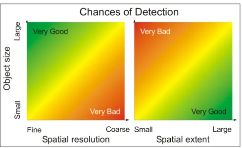
Figure 2.11 – The chances of object detection based on the spatial scale.
Figure 2.12 – The importance of accuracy and precision. The left graphs present a target and distribution, which is both accurate and precise. The middle graph represents poor accuracy but good precision and the right hand graph shows both poor accuracy and precision.
Figure 3.1 – A graphical representation of the regionalized variable (top graph), the Random Variable (RV) (middle graph) and the Random Function (RF) (bottom graph). Each square represents a recorded value within an image.
Figure 3.2 – Any translation of the data within the area deemed stationary would result in the same distribution.
Figure 3.3 – Pairs of pixels representing the distance classes that would be used to compute the variogram along a line of pixels.
Figure 3.4 – An idealised variogram. The variogram is a graph (and/or formula) describing the expected difference in value between pairs of pixels.
Figure 3.5 – The sequential gaussian simulation algorithm represented graphically. Figure 4.1 – A diagram of the proposed methodology. The three phases are related to the different types of information used to generate the finer spatial resolution imagery.
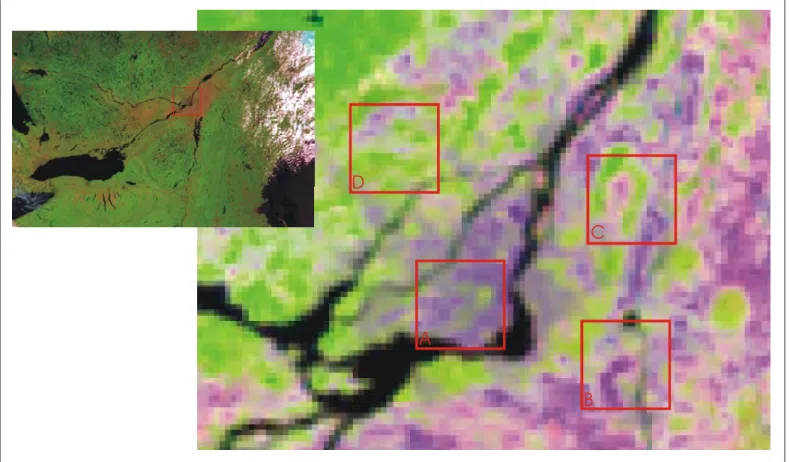
Figure 4.2 – SPOT 4 VGT imagery. Upper left inset presents the areal extent that can be sensed by the VGT sensor (about 2200 km). The central image presents a magnification of the island of Montreal and surrounding areas that is approximately equal to the extent covered by a single SPOT 4 HRVIR image. The red squares each encompass a study area 15 x 15 km denoted as study areas A through D.
Figure 4.3 – SPOT 4 HRVIR imagery of the four study sites denoted A through D. Figure 4.4 – RADARSAT-1 ScanSAR wide beam mode imagery. Upper left inset presents the full RADARSAT-1 image in ScanSAR wide beam mode. The image was recorded while ascending and produced using the w1, w2, s5 and s6 beam modes. Each of the images (A through D) covers the same area as that of the HRVIR and VGT image subsets.
Figure 4.5 – The LVM and co-simulation node configurations. The LVM case has a background value for all the nodes that are within a single VGT pixel while the co-simulation case places the VGT pixel value as a central node within a single VGT pixel extent.
Figure 5.1 – Histogram of the study sites A (left side) and B (right side). All three spectral channels are shown for each image (from top to bottom).
Figure 5.2 – Histogram of the study sites C (left side) and D (right side). All three spectral channels are shown for each image (from top to bottom).
Figure 5.3 – The experimental variogram was computed for all the coarse spatial resolution images in two directions: north-south (0°) and east-west (90°), and in all directions (omni-directional variogram, circular arrow). The variogram legend is found on the right side of the figure.
Figure 5.4 – Computed variograms for sites A (left side) and B (right side). The variograms were computed on each channel in 2 directions (north-south and east-west) and in all directions (omni-directional variogram). Note that the abscissa scale is not constant.
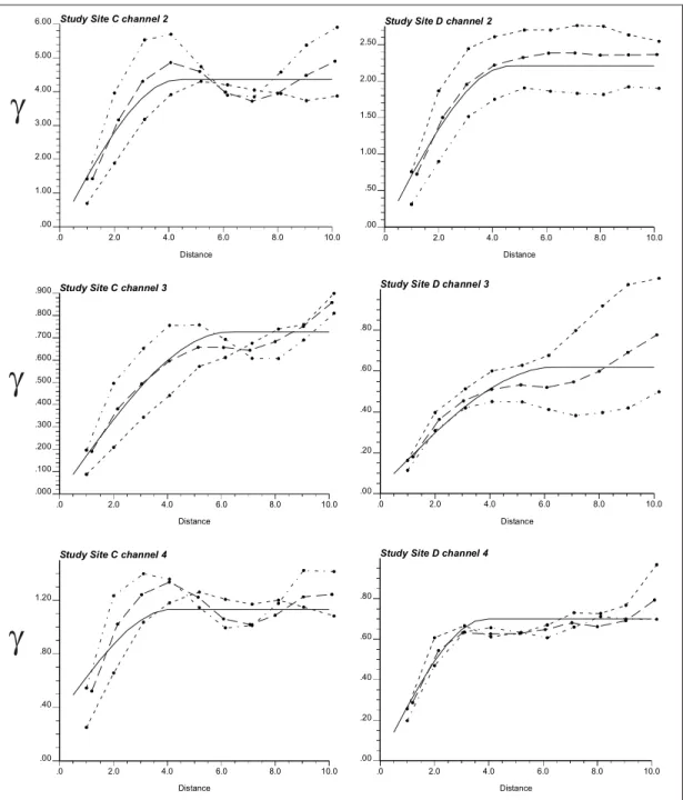
Figure 5.5 – Computed variograms for sites C (left side) and D (right side). The variograms were computed on each channel in 2 directions (north-south and east-west) and in all directions (omni-directional variogram). Note that the abscissa scale is not constant.
Figure 5.6 – Phase I generated finer spatial resolution images using sequential gaussian simulation and the LVM option for study sites A through D.
Figure 5.7 – Phase I computed histograms based on the generated finer spatial resolution imagery with the LVM option. Study sites A (left side) and B (right side) are presented with all image channels (from top to bottom).
Figure 5.8 – Phase I computed histograms based on the generated finer spatial resolution imagery with the LVM option. Study sites C (left side) and D (right side) are presented with all image channels (from top to bottom).
Figure 5.9 – The variograms of residuals based on the study sites A and B VGT images.
Figure 5.10 – The variograms of residuals based on the study sites C and D VGT images.
Figure 5.11 – Phase I generated finer spatial resolution images using sequential gaussian simulation and the LVM option with the variogram of residuals for study sites A through D.
Figure 5.12 – Phase I generated finer spatial resolution images using the sequential gaussian algorithm with the co-simulation option.
Figure 5.13 – Single realisation co-simulation histograms of the spectral channels based phase I input parameters for study sites A (left side) and B (right side).
Figure 5.14 – Single realisation co-simulation histograms of the spectral channels based on phase I input parameters for study sites C (left side) and D (right side). Figure 5.15 – Phase I E-type statistic presented in false colour based on 50 realisations.
Figure 5.16 – Phase I 10th percentile statistic presented in false colour based on 50 realisations.
Figure 5.17 – Phase I median statistic presented in false colour based on 50 realisations.
Figure 5.18 – Phase I 90th percentile statistic presented in false colour based on 50 realisations.
Figure 5.19 – Histograms computed from the E-type estimate images based on the set of 50 realisations for sites A (left side) and B (right side).
Figure 5.20 – Histograms computed from the E-type estimate images based on the set of 50 realisations for sites C (left side) and D (right side).
Figure 5.21 – Histograms computed from the 10th percentile images based on the set of 50 realisations for sites A (left side) and B (right side).
Figure 5.22 – Histograms computed from the 10th percentile images based on the set of 50 realisations for sites C (left side) and D (right side).
Figure 5.23 – Histograms computed from the median images based on the set of 50 realisations for sites A (left side) and B (right side).
Figure 5.24 – Histograms computed from the median images based on the set of 50 realisations for sites C (left side) and D (right side).
Figure 5.25 – Histograms computed from the 90th percentile images based on the set of 50 realisations for sites A (left side) and B (right side).
Figure 5.26 – Histograms computed from the 90th percentile images based on the set of 50 realisations for sites C (left side) and D (right side).
Figure 6.1 – Computed histograms based on the HRVIR images of study sites A (left side) and B (right side).
Figure 6.2 – Computed histograms based on the HRVIR images of study sites C (left side) and D (right side).
Figure 6.3 – Legend for the experimental variograms based on the HRVIR imagery (figures 6.4 and 6.5).
Figure 6.4 – Computed experimental and model variograms based on the HRVIR fine spatial resolution imagery for study sites A (left side) and B (right side). Distance is
shown in pixels where 1 pixel is equal to 20 m (Note the abscissa axis is not constant).
Figure 6.5 – Computed experimental and model variograms based on the HRVIR fine spatial resolution imagery for study sites C (left side) and D (right side). Distance is shown in pixels where 1 pixel is equal to 20 m (Note the abscissa axis is not constant).
Figure 6.6 – Phase II generated finer spatial resolution imagery using the LVM option.
Figure 6.7 – Phase II single realisation co-simulated imagery of study sites A through D.
Figure 7.1 – Histogram of the RADARSAT ScanSAR wide imagery.
Figure 7.2 – Generated finer spatial resolution imagery conditioned with SAR imagery.
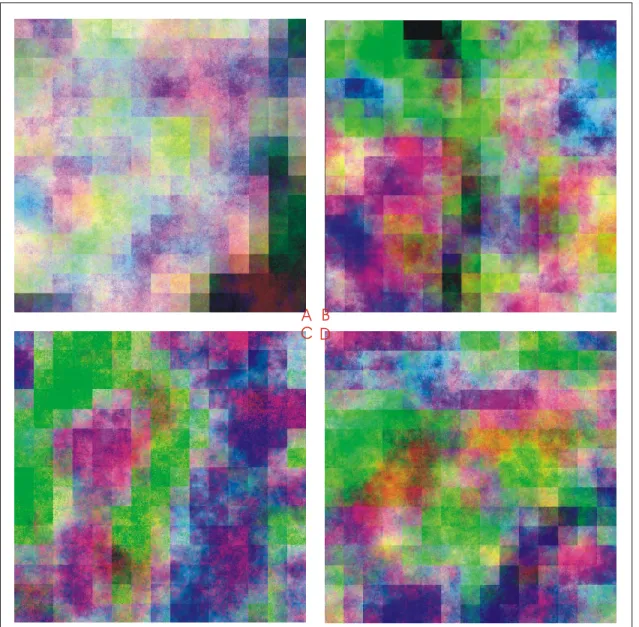
Figure 7.3 – Generated imagery computed from 50 realisations using the E-type estimate and phase III input parameters for study sites A through D.
Figure 8.1 – Three-dimensional representation of the spectral groupings in spectral feature space after segmentation based on the K-means algorithm. The results shown are for study site A and a maximum of 16 groups.
Figure 8.2 – K-means segmentation results for phase I and II statistical images. The results shown are for study site A and a maximum of 16 groups.
Figure 8.3 – K-means segmentation phase III results for study site A. The results shown are for study site A and a maximum of 16 groups.
Figure 8.4 – Three-dimensional representation of the spectral groupings in spectral feature space after segmentation based on the K-means algorithm. The results shown are for study site A and a maximum of 10 groups.
Figure 8.5 – K-means segmentation results for phase I and II statistical images. The results shown are for study site A and a maximum of 10 groups.
Figure 8.6 – K-means segmentation phase III results for study site A. The results shown are for study site A and a maximum of 10 groups.
Figure 8.7 – Three-dimensional representation of the spectral groupings in spectral feature space after segmentation based on the K-means algorithm. The results shown are for study site B and a maximum of 16 groups.
Figure 8.8 – K-means segmentation results for phase I and II statistical images. The results shown are for study site B and a maximum of 16 groups.
Figure 8.9 – K-means segmentation phase III results for study site A. The results shown are for study site B and a maximum of 16 groups.
Figure 8.10 – Ranked spectral segments based on the pixel count. The results shown are for study site A and a maximum of 16 groups.
Figure 8.11 – Classified spectral segments based on percent cover of study site A with 16 classes (single realisation images).
Figure 8.12 – Classified spectral segments based on percent cover of study site A with 16 classes (E-type estimate and median images).
Figure 8.13 – Classified spectral segments based on percent cover of study site A with 16 classes (10th and 90th percentile images).
Figure 8.14 – Ranked spectral segments based on the pixel count. The results shown are for study site A and a maximum of 10 groups.
Figure 8.15 – Classified spectral segments based on percent cover of study site A with 10 classes (single realisation images).
Figure 8.16 – Classified spectral segments based on percent cover of study site A with 10 classes (E-type estimate and median images).
Figure 8.17 – Classified spectral segments based on percent cover of study site A with 10 classes (10th and 90th percentile images).
Figure 8.18 – Ranked spectral segments based on the pixel count. The results shown are for study site B and a maximum of 16 groups.
Figure 8.19 – Classified spectral segments based on percent cover of study site B with 16 classes (single realisation images).
Figure 8.20 – Ranked spectral segments based on the pixel count. The results shown are for study site B and a maximum of 10 groups.
Figure 8.21 – Classified spectral segments based on percent cover of study site B with 10 classes (single realisation images).
Figure 8.22 – CLI vectors superimposed on the spectrally segmented images of study site A based on 16 clusters.
Figure 8.23 – The distribution of spectral segments within the built-up land-cover class for study site A based on 16 clusters.
Figure 8.24 – The distribution of spectral segments within the water land-cover class for study site A based on 16 clusters.
Figure 8.25 – CLI vectors superimposed on the spectrally segmented images of study site B based on 16 clusters.
Figure 8.26 – The distribution of spectral segments within the built-up land-cover class for study site B based on 16 clusters.
Figure 8.27 – The distribution of spectral segments within the water land-cover class for study site B based on 16 clusters.
Figure 8.28 – The distribution of spectral segments within the pasture land-cover class for study site B based on 16 clusters.
Figure 8.29 – The distribution of spectral segments within the woodland land-cover class for study site B based on 16 clusters.
Figure 8.30 – CLI vectors superimposed on the spectrally segmented images of study site C based on 16 clusters.
Figure 8.31 –The distribution of spectral segments within the pasture land-cover class for study site C based on 16 clusters.
Figure 8.32 – The distribution of spectral segments within the woodland land-cover class for study site C based on 16 clusters.
Figure 8.33 – CLI vectors superimposed on the spectrally segmented images of study site D based on 16 clusters.
Figure 8.34 – The distribution of spectral segments within the woodland land-cover class for study site D based on 16 clusters.
Figure 8.35 – Woodland vectors superimposed on the spectrally segmented images of study site D based on 16 clusters (1:50 000 map scale).
Figure 8.36 – The distribution of spectral segments within the woodland land-cover class for study site D based on 16 clusters (1:50 000 map scale).
Figure 8.37 – Proposed validation procedure for comparing generated finer spatial resolution images to a validation data set.
Glossary
AVHRR – Advanced Visible High Resolution Radiometer BOREAS – BOReal Ecosystem-Atmosphere Study
CDF – cumulative distribution function
CCDF – conditional cumulative distribution function
CORINE – Co-Ordination of Information on the Environment EM – Electromagnetic (refers to the Electromagnetic spectrum) DN – Digital Number
IFOV – Instantaneous Field of View
VGT – VEGETATION sensor onboard the SPOT 4 satellite
HRVIR – High Resolution Visible Infrared sensor onboard the SPOT 4 satellite Land-cover – the composition and characteristics of land surface elements NIR – Near Infrared
NOAA – National Oceanic and Atmospheric Administration OK – Ordinary Kriging
PSF – Point Spread Function RF – Random Function RV – Random Variable
Scaling-up (or bottom up) – Aggregation process where the original spatial data are reduced to a smaller number of data units.
Scaling-down (or top down) – the reverse of scaling-up, i.e. increasing the number of data units based on a limited data set.
SAR – Synthetic Aperture Radar SD – Standard Deviation
SWIR – Short Wave Infrared
SGSIM – Sequential Gaussian Simulation
Acknowledgements
Dr. François Cavayas is my director, employer and friend. I wish to thank him for the support that he gave me throughout these last four years. His encouragement and friendship allowed me to finish without losing my mind. A special thanks to Dr. Marc D’Iorio of the Canada Centre for Remote Sensing for co-directing and asking those special questions that everyone else seemed to forget.
This thesis would not be possible without data, which was made possible by a grant from the EODS (Earth Observation Data Sets) program, Canada Centre for Remote Sensing. Additional support was received from the FCAR Bourses de recherche en milieu pratique (Fonds FCAR-MRST) of the government of Québec which allowed me to work with Dr. Langis Gagnon at the CRIM (Centre de Recherche en Informatique de Montréal).
A special thank you to all those who in my final year (the year that I wrote this thesis) gave me a roof over my head. I will never forget the graciousness that you showed me and you are always welcome to visit (Natasha, Pierre, Bronek, Genevieve, Gabriel, and François).
Scientists and policy-makers rely upon satellite based remotely sensed data to extract pertinent information relating to the state of the environment. At the global scale, categorising geographic space into broad land-cover classes (e.g. forest, urban, etc.) and monitoring their changes over time are important because land-cover distribution and change are inputs to many studies including desertification, greenhouse effects, etc. Projects such as TREES (TREES 1999) or NASA's Landsat Pathfinder Humid Tropical Deforestation Project (UMD 1998) use estimates of the total tropical forest cover across the globe to help measure changes caused by natural and anthropogenic disturbances over time. Land-cover can also be used as a surrogate for specific parameters (e.g. plant biomass or canopy conductance) that cannot be measured directly over large regions (Cihlar et al. 1997) as in the case of the BOREAS project that deals with ecosystem-atmosphere interactions (BOREAS; Sellers et al. 1995). Future monitoring will support governments for environmental action. The Kyoto protocol (UNFCCC 2001) calls for better forest management and countries are rewarded or penalised depending on the state of their forests. Such monitoring demands accuracy in order to make sure that protocol compliance be rewarded and non-compliance be penalised. Uncertainties in such situations (Townshend et al. 1992) provide political loopholes and no means of upholding the law because verification is erroneous.
Acquiring data on the state of and changes in land-cover at the global scale however, is not an easy task. The most suitable satellite imagery provides large area
coverage while maintaining an adequate spatial resolution for land-cover characterization. The extent of the recorded image determines the total ground scene area that can be sensed and must be large enough to supply a “snapshot” in time of the land-cover state of the whole Earth. A large extent also allows for a finer temporal resolution providing important monitoring information that can be used to separate seasonal trends in land-cover change from disturbances and modifications. In a practical sense, optical data benefits from such a fine temporal resolution because cloud cover and atmospheric effects, in general, are reduced.
However, such an ideal remote sensor does not exist because there is always a trade-off between extent of coverage and fineness of the spatial resolution. Over the last 20 years, experimentation with the NOAA AVHRR series of satellite based sensors (about 2000 km of spatial coverage at 1 km spatial resolution and daily coverage) has shown the difficulty of applying coarse spatial resolution optical imagery specifically to the extraction of thematic content and estimating its proportions (Justice et al. 1989, Townshend et al. 1991, Townshend et al. 1992, Townshend et al. 1994, Mayaux and Lambin 1995; 1997). The fact that recorded observations and derived conclusions are scale dependent is well known (Gosz 1986, Addicott et al. 1987). The certainty in identifying ground scene composition and characteristics increases as the scale of observation (i.e. resolution and extent of image data) provides the necessary details at the scale of inference (i.e. resolution and extent of extracted information). Thus, a general practice applied today to obtain an exact characterisation of broad land-cover categories is to classify fine spatial resolution satellite data and scale-up. The scaling-up procedure involves aggregating
the land-cover classes based on cartographic generalisation criteria e.g. at what map scale will side roads still be shown. The European CORINE land-cover program is based on the principle of cartographic generalisation and in Canada this principle will also be utilised to meet the Kyoto protocol requirements. However, such an approach is very time consuming and does not meet the fine temporal revisit criterion.
In order to extract the same broad land-cover categories from satellite based optical coarse spatial resolution imagery the opposite procedure would need to be applied: scaling-down. Scaling-down is more problematic because less information is available at the start. Technological advances provide better optical coarse spatial resolution imagery and favourable experimental conditions to examine the feasibility of such a scaling-down procedure. In fact the VGT and the HRVIR sensors on board the SPOT-4 satellite provides respectively large extent/coarse spatial resolution imagery and small extent/fine spatial resolution imagery that can be recorded in parallel (VEGETATION 1999). Thus it is possible to generate data sets of the same area of interest at both fine and coarse spatial resolutions under the same external conditions (time of the day, atmospheric and solar illumination conditions). In addition, the availability of SAR satellite images with relatively large area coverage (500 km x 500 km) and medium spatial resolution (<100 m), such as the ScanSAR wide mode of RADARSAT-1, could be introduced as an independent source of information into this scaling-down procedure. A scaling-down procedure could be realised and the quality of the scaled-down imagery in terms of land-cover characterization constitute the core of this thesis. Geostatistical stochastic imaging
techniques are the privileged tool for such a procedure for the reasons explained in the next section.
1.1 Available Techniques
The existing techniques that aim to improve the information extraction potential from coarse spatial resolution images introduce “exogenous image data”. These techniques can be separated into two general categories (table 1.I). Image enhancement tries to provide a visually more appealing product while error correction attempts to correct land-cover estimates.
Table 1.I – Various approaches to improve image quality and derived information.
Goal Method References
Image
Enhancement
Fusion Carper et al. 1990; Chavez et al. 1991; Pohl and
Van Genderen 1998; Ranchin and Wald 2000; Liu 2000; Del Carmen Valdes and Inamura 2001 Error
Correction Regression Kong and Vidal-Madjar 1988; Foody 1994; Oleson et al. 1995; Mayaux and Lambin 1995; Fazakas and Nilsson 1996; Maselli et al. 1998 Modelling Iverson et al. 1989; Zhu and Evans 1992; Cross
et al. 1991; Kerdiles and Grondona 1995;
Ouaidrari et al. 1996; Atkinson et al. 1997
Image enhancement (table 1.I – first row) is primarily achieved through fusion techniques. Fusion techniques use fine spectral/coarse spatial resolution imagery that is combined with coarse spectral/fine spatial-resolution imagery to obtain an image with the finest spectral/spatial resolution combination.
Error correction procedures are often based on either regression or modelling. When regression is used (table 1.I – middle row), relationships between samples of fine spatial resolution parameters and the matching coarse spatial resolution parameters are computed. These relationships are then extrapolated over regions where only the coarse spatial resolution parameter is present to estimate the fine spatial resolution parameters.
Modelling can encompass a large number of techniques. One of the more used techniques is mixture modelling (table 1.I – last row). Mixture modelling is based on the assumption that the measured spectral response from a particular image pixel is related to the mixture or patterns of cover types in that location.
The afore mentioned techniques, however, do not provide all the necessary solutions to improve image data quality gathered over large regions. Image fusion necessarily requires a fine spatial/coarse spectral resolution image as well as a coarse spatial/fine spectral resolution image that both cover the same region. Monitoring large regions using this technique is therefore unfeasible because fine spatial resolution imagery is usually not available. The regression and modelling techniques require fine spatial resolution image samples for calibration. The larger the area under investigation, the more sample sites are required. Furthermore, the complexity of the ground scene is a determining factor in the required number of sample and validation sites and thus the number of required fine spatial resolution samples increases as spatial heterogeneity increases.
Previous studies showed that coarse spatial resolution optical imagery (NOAA AVHRR) had quantifiable spatial variability based on the variogram (e.g. Gohin 1989, Bielski 1997). This information together with image statistics could be the input for various geostatistical methods (i.e. kriging or stochastic imaging) to generate finer spatial resolution imagery.
Geostatistical methods, which were originally developed for the mining industry in the 1950’s, were later introduced into the remote sensing context in the late 1980’s by Woodcock et al. (1988a, 1988b). Many remote sensing studies and applications have since used geostatistics and some typical studies are presented in table 1.II. However, no attempt has been documented until now to generate a finer spatial resolution image using geostatistical techniques. More importantly, no attempt has been made to examine whether such a scaling-down procedure can generate an image whose spectral characteristics approach those of a fine spatial resolution image that is considered optimal for land-cover classification at the regional scale.
Table 1.II – A listing of geostatistical applications in the remote sensing context. Curran and Dungan
1988
Used the semi-variogram to isolate sensor noise and remove intra-pixel variability
Gohin 1989 Used the variogram and co-variogram to compare sea surface temperatures taken in situ and from satellites to evaluate the importance of spatial structures in the data and instrument error. Webster et al. 1989 Variogram was used to design sampling schemes for estimating
the mean to meet some specified tolerance expressed in terms of standard error.
Atkinson et al. 1990 Selection of sufficient image data for compressed storage.
Cohen et al. 1990 Computed semivariograms on images of a variety of Douglas-fir stands and found relationships between patterns in stand structure, canopy layering and percent cover.
Bhatti et al. 1991 Interpolated ground measurements of soil properties and crop yield over large areas combined with Landsat TM data using kriging and co-kriging.
Atkinson et al. 1992 Applied co-kriging using ground based radiometry. D'Agostina and
Zelenka 1992
Applied the co-kriging technique to two available information sources to reduce the estimation error.
Dungan et al. 1994 Provided examples of kriging and stochastic imaging to map vegetation quantities using ground and image data.
Lacaze et al. 1994 Compared variogram of different Mediterranean environments based on images from a variety of sources (air and satellite based).
Rossi et al. 1994 Interpolated land-cover classes found under the clouds with kriging.
Atkinson and Curran
1995 Evaluation of the relation of size of support with the precision of estimating the mean of several properties using kriging. St-Onge and Cavayas
1995
Used the directional variogram from high spatial resolution images to estimate height and stocking of forest stands.
Eklundh 1995 Noise estimation in AVHRR data using the nugget variance. Lark 1996 Computed semi-variance in a local window for lags of different
length and direction to discriminate land-cover classes.
Van der Meer 1996 Development of indicator kriging based classification technique for hyperspectral data.
Curran and Atkinson
1998 Presented overview of geostatistics in remote sensing with examples. Dungan 1998 Compared regression, co-kriging and stochastic imaging
techniques to generate maps based on sampled imagery.
Wulder et al. 1998 Used variogram model parameters to compute the semivariance moment texture as a surrogate of forest structure to related LAI and vegetation indices.
Atkinson and Emery 1999
Explored the spatial structure of different bands using the variogram.
Initial attempts by the author to generate finer spatial resolution images were done using the kriging interpolator with unsatisfactory results (Bielski and Cavayas 1998, Bielski 1999). Kriging proved to be inadequate because the interpolation algorithm generated smoothed images whose overall statistics did not reproduce the anticipated results at the finer spatial resolution. These difficulties could in principle be overcome with the application of the geostatistical stochastic imaging technique (Dungan 1998, Goovaerts 2000) because the simulated data is not smoothed.
1.2 Objectives and Hypotheses
An attempt is made in this thesis to establish a practical procedure to generate finer spatial resolution imagery based on coarse spatial resolution optical imagery and stochastic imaging. This generated imagery could then provide a better land-cover characterization than the original imagery could. The generated finer spatial resolution imagery would provide a finer unit of measurement (finer spatial resolution) and more spectral variability to discern different land-cover types.
The specific objectives of the study are as follows:
- analyse the ways that experimental variograms and other statistical parameters extracted from the sole coarse spatial resolution imagery could be used as a support for generating finer spatial resolution imagery;
- analyse the possibility of using information provided by non optical sensors (SAR imagery);
- validate the various generated images in terms of location and possible class labels.
The working hypotheses based on previous personal work are:
- that the coarse spatial resolution imagery preserves enough information to generate new data with similar spectral characteristics compared to a finer spatial resolution imagery;
- that geostatistical theory as well as the stochastic imaging techniques can be used to change the spatial scale of remotely sensed imagery;
- that SAR imagery can provide spatial location information to enhance the generated optical images;
- that an automatic segmentation algorithm is applicable to synthetic multi-spectral imagery in order to obtain meaningful land-cover classes.
A tool able to zoom-in (or out) on available coarse spatial resolution imagery based on geostatistical knowledge could provide the data necessary to fill in the gaps between unavailable finer resolution sensor data. This approach presented here concentrates on the structure of the data itself and generates image data in the same spectral bands as those found in the original coarse spatial resolution imagery. The procedure itself is based on generating data with similar characteristics as that of finer spatial resolution imagery and information extraction therefore becomes a secondary step. Information extraction as a secondary step facilitates the creation or loss of information rather than modelling how land-cover objects appear or disappear depending on the scale of observation. A reliable segmentation or supervised classification method thus remains an integral part of the information extraction procedure.
1.3 Originality and Contribution of the Thesis
The novel idea behind the approach presented in this thesis is to apply a stochastic imaging technique to generate imagery at a finer spatial resolution. The stochastic imaging algorithm explored for this purpose was the sequential gaussian simulation algorithm. In addition, both the locally varying mean (LVM) and co-simulation techniques were tested. Theoretically such an approach could be applied without recourse to any spatial data set. However, the goal is to generate a finer spatial resolution data set based solely on available coarse spatial resolution imagery whose characteristics are similar to a fine spatial resolution image that could be acquired in reality. Furthermore, the emphasis is placed on modelling the change in the overall statistics of the images rather than modelling the manner in which land-cover classes change over different spatial scales. Consequently, applying traditional segmentation techniques and classification strategies to generated finer spatial resolution optical imagery is a new tactic.
Testing the viability of zooming-in to coarse spatial resolution data by means of geostatistical stochastic imaging is important because of the possibility of increasing certainty about derived information. This particular approach could increase certainty through the availability of finer spatial resolution data. Use of finer spatial resolution data means that the scale of observation is closer to that required by the user (scale of inference) and should therefore reduce error. The usefulness of the resulting generated finer spatial resolution image data however, is entirely dependent
on whether the theory behind the stochastic imaging algorithms is sound. Success in this work would allow researchers to generate finer spatial resolution imagery for global studies based on coarse spatial resolution data. As such, historical AVHRR imagery can also be re-examined to improve land-cover assessment.
Another novelty of this thesis is the inclusion of SAR imagery into the scaling-down process. SAR data differs from optical data in that the sensor is active as well as the fact that it records wavelengths in the cm range. The benefit of the SAR data to generating finer spatial resolution imagery is that it can provide spatial location information that is lacking in the original coarse spatial resolution data.
As mentioned earlier, satellite based remote sensing image data are available in a multitude of configurations because no single sensor can provide the user with all the information associated with a specific ground scene. It is expected that the results of this research will give increased confidence in using coarse spatial resolution images for deriving and estimating land-cover at the regional scale of observation.
1.4 Structure of the Thesis
The thesis is subdivided into nine chapters. Chapter 2 discusses the role of resolution and extent in deriving information from remotely sensed data. The remotely sensed data chosen for this investigation were image data that recorded in either the optical or microwave region of the EM spectrum. This choice rests on the fact that these are presently the two most common sensor configurations for satellite
remote sensing platforms. A discussion of the spatial, spectral, radiometric and temporal scales related to these types of sensors is also presented. The scale of observation is based on the sensor characteristics while the scale of inference pertains to the scale at which conclusions are made (Csillag et al. 2000). The final goal of any remote sensing campaign is to extract pertinent information from the image data. The relationship between the scale of observation and the scale of inference determines the certainty with which one can draw conclusions but this relationship is usually unknown.
Remotely sensed imagery is a regionalised variable and chapter 3 provides a practical explanation of the geostatistical tools applied including the experimental variogram, the model variogram, regularisation and stochastic imaging. Specifically, the sequential gaussian simulation algorithm was chosen for this research because of its ease of implementation, speed and suitability for the available data. Both LVM and co-simulation implementations were tested.
The methodology as well as the data are presented in chapter 4. Chapters 5 to 7 describe the three phases of the experiment. Each phase was designed to introduce more information into stochastic imaging process. Phase I generates finer spatial resolution imagery based on coarse spatial resolution statistics and data. Phase II generates finer spatial resolution imagery based on derived fine spatial resolution statistics and coarse spatial resolution data. The final phase uses the same information as phase II to which it incorporates SAR imagery to better localise spectral objects. In chapter 8, each of the generated images is then segmented in order to analyse their
usefulness in deriving and estimating land-cover at the regional scale of observation. Finally, the resulting spectral segments are validated with Canadian Land Inventory (CLI) data. Chapter 9 presents a summary discussion of the work as well as the conclusions.
The remotely sensed image itself is a recording of spectral measurements arranged in space. These data are ultimately used to derive land-cover information about a recorded ground scene. The data itself and the scale of observation directly determine the information content and is based on the spatial, spectral, radiometric and temporal characteristics. In digital form, the data are easily manipulated and algorithms help enhance and automate the information extraction process. The following sections discuss the remotely sensed image characteristics and the difficulties in extracting the desired information, especially from coarse spatial resolution images.
2.1 Remotely Sensed Image Characteristics
An important characteristic of remotely sensed image data quality is resolution (or the overall fineness of detail characterising the image) and extent. The resolution is the smallest unit from which a meaningful measurement can be recorded. Qualitatively it is described as either fine or coarse. The extent refers to the limits of the resolution characteristic in question with small and large describing its qualities. The two are inseparable and context dependent.
2.1.1 Spatial resolution
The most obvious characteristic of any remotely sensed image is spatial resolution. Optical sensors record reflected energy in the visible and reflective IR
regions of the EM spectrum (0.4 – 2.5 µm). The spatial resolution of these sensors can be defined by
- the geometrical properties of the imaging system, - the ability to distinguish between point targets,
- the ability to measure the spectral properties of small targets and,
- the ability to measure the periodicity of repetitive targets (separability) (Mather 1987),
- dwell time in new sensors.
The IFOV of a sensor is the ground scene area contributing to a single measurement as defined by the sensor’s aperture (geometric properties) (figure 2.1). The IFOV is the area on the ground that is viewed by the instrument from a given altitude at any given instant in time. The equation
D = H * b
computes the spatial resolution (diameter D) of an image knowing the height of the sensor (H) and the IFOV in radians (b). The resulting image data is affected by the IFOV because for a given flying height, the IFOV is positively related to the sampled ground extent but negatively related to the spatial resolution (Curran 1985).
The point spread function (PSF) of a sensor, or the distribution of intensity from a single point source, influences the spatial resolution through the sensor’s ability to distinguish between point targets. The presence of relatively bright or dark objects within the IFOV of the sensor will increase or decrease the amplitude of the
PSF so as to make the observed radiance either higher or lower than that of the surrounding areas. Therefore, objects that are smaller than the IFOV spatial resolution of the sensor can still be detected (e.g. small rivers in the NIR band).
H e ig ht ( H ) b IFOV Diameter (D)
Figure 2.1 – Spatial resolution based on the geometric properties of the imaging system where D is the diameter of the ground sampling element in metres, H is the height of the sensor and b is the IFOV in radians.
The Effective Resolution Element (ERE) is a measure of spatial resolution based on the size of an area for which a single radiance value can be assigned with reasonable assurance that the response is within 5 % of the value representing the actual relative radiance. The Effective Instantaneous Field of View (EIFOV) is based on the spatial frequency of distinguishable objects. This measure is usually based on
theoretical targets and therefore is likely to exceed the performance of an instrument in actual applications (Mather 1987).
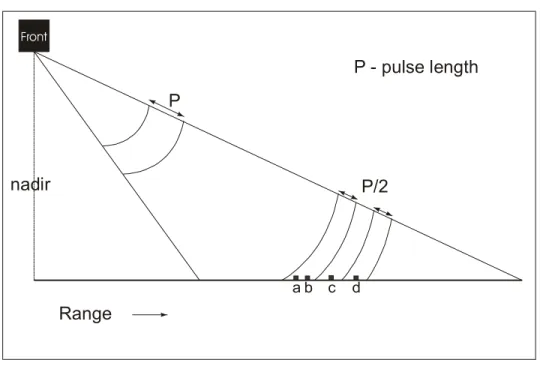
Optical sensors depend on reflected sunlight (passive system) while a radar sensor sends and receives energy pulses (active system) in the millimetre to metre range. The spatial resolution of a radar system is based on the ability of its antenna to identify two closely spaced targets as separate points, i.e. the points will appear on the image as two distinct dots. For example, if a particular radar system is able to distinguish two closely spaced objects as separate; a lower resolution system may only distinguish one object. Radar spatial resolution is measured in both the azimuth (i.e. flight) and range (i.e. side looking) directions and is controlled by the radar system and antenna characteristics. The signal pulse length (figure 2.2) and the beam width (figure 2.3) thus control the radar systems spatial resolution. The signal pulse length dictates the spatial resolution in the direction of energy propagation where shorter pulses will result in a finer spatial resolution in the range direction. The width of the beam dictates the resolution in the azimuth direction. The beam width is directly proportional to the radar wavelength and is inversely proportional to the length of the transmitting antenna. This means that spatial resolution deteriorates as the distance increases from the antenna with respect to the target. Therefore a long radar antenna is required to achieve finer spatial resolution in the flight direction. Since satellites are very far from their targets, in theory this would require the system to carry an enormous antenna.
P nadir P/2 Range a b c d P - pulse length Front
Figure 2.2 – Spatial resolution in the range direction for a radar system.
Azimuth a b c d Antenna beam width R ange TOP
Figure 2.3 – Spatial resolution in the azimuth direction for a radar system.
In order to circumvent the need for a very long antenna, the Synthetic Aperture Radar (SAR) was developed. SAR uses a short antenna that can simulate a much larger antenna through modified data recording and signal processing techniques. Signal processing techniques also allow azimuth resolution to be independent of range resolution (CCRS 2001).
Figure 2.4 presents a diagram of the geometry of a radar system. The diagram indicates that the range resolution is divided into two different types of spatial resolutions, slant (e) and ground (a) resolutions.
Y X Y X a g b Hn e S φn φf β Hn - flying height - depression angle
- near edge incidence angle - far edge incidence angle S - slant range
β φ φnf
g - ground range
a - ground range resolution (x) b - azimuth resolution (y) e - slant range resolution
Figure 2.4 – The geometry of a radar system.
The range resolution is determined by the frequency bandwidth of the transmitted pulse and thus by the duration (width) of the range-focused pulse. Large bandwidths yield small focused pulse widths. The range resolution of imaging radars depends on signal pulse length and therefore the actual distance resolved is that
distance between the leading and the trailing edge of the pulse. These pulses can be shown in the form of signal wave fronts propagating from the sensor (figure 2.4 (e)). When these wave front arcs are projected to intersect a flat earth surface, the resolution distance in ground range is always larger (coarser) than the slant range resolution (figure 2.4 (a)). The resolution in the azimuth direction is theoretically one-half of the radar antenna.
The SAR system collects signal history that is not in image format. The raw data is impossible to interpret visually and therefore must be digitally processed in a procedure called compression. Compression converts the history in the range and azimuth directions to a two-dimensional grid format whose basic subdivision is the slant range and zero Doppler resolution cell. This cell relates to the smallest ground area for which a reflection intensity value was calculated during processing (single look). A single look is prone to excessive speckle and therefore the signals are usually processed using several looks. This degrades the spatial resolution of the generated image but attenuates the speckle.
Another type of spatial resolution pertains to the manner in which digital imagery is viewed. Digital imagery is most often displayed on a computer screen where the pixel, or picture element, is the smallest element able to display data. This pixel has nothing to do with the physical attributes recorded by the sensor and therefore, the on-screen spatial resolution of an image can be changed effortlessly. The term ‘pixel’ also pertains to the area on the ground represented by the data values (Colwell 1983) in the remote sensing context.