HAL Id: hal-01087363
https://hal.inria.fr/hal-01087363
Submitted on 26 Nov 2014
HAL is a multi-disciplinary open access
archive for the deposit and dissemination of
sci-entific research documents, whether they are
pub-lished or not. The documents may come from
teaching and research institutions in France or
abroad, or from public or private research centers.
L’archive ouverte pluridisciplinaire HAL, est
destinée au dépôt et à la diffusion de documents
scientifiques de niveau recherche, publiés ou non,
émanant des établissements d’enseignement et de
recherche français ou étrangers, des laboratoires
publics ou privés.
Transition Systems
Uli Fahrenberg, Kim Guldstrand Larsen, Axel Legay, Louis-Marie Traonouez
To cite this version:
Uli Fahrenberg, Kim Guldstrand Larsen, Axel Legay, Louis-Marie Traonouez.
Parametric and
Quantitative Extensions of Modal Transition Systems. FPS@ETAPS, Apr 2014, Grenoble, France.
�10.1007/978-3-642-54848-2_6�. �hal-01087363�
of Modal Transition Systems
Uli Fahrenberg1
, Kim G. Larsen2
, Axel Legay1
, and Louis-Marie Traonouez1
1
Inria / IRISA, Rennes, France
2
Aalborg University, Aalborg, Denmark
Abstract. Modal transition systems provide a behavioral and composi-tional specification formalism for reactive systems. We survey two exten-sions of modal transition systems: parametric modal transition systems for specifications with parameters, and weighted modal transition systems for quantitative specifications.
1
Introduction
Modal transition systems [21, 23] provide a behavioral and compositional specifi-cation formalism for reactive systems. They grew out of the notion of relativized bisimulation [20], which allows for simple specifications of components by allowing the notion of bisimulation to take into account the restricted use that a given component may have in its context.
A modal transition system is essentially a (labeled) transition system, but with two types of transitions: so-called may-transitions which any implementation may (or may not) have, and must-transitions which any implementation is required to have. In fact, ordinary labeled transition systems (or implementations) are modal transition systems where the set of may- and must-transitions coincide. Modal transition systems come equipped with a bisimulation-like notion of (modal) refinement, reflecting that the more must-transitions and the fewer may-transitions a modal specification has the more refined and closer to a final implementation it is.
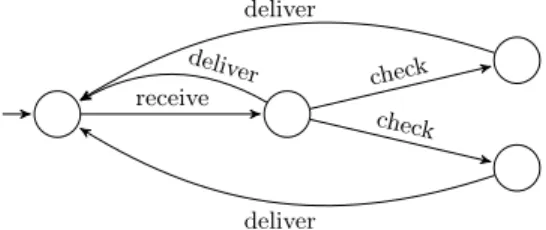
Example 1. Consider the modal transition system shown in Fig. 1 which models
the requirements of a simple email system in which emails are first received and then delivered; must- and may-transitions are represented by solid and dashed arrows, respectively. Before delivering the email, the system may check or process the email, e.g. for encryption or decryption, filtering of spam emails, or generating automatic answers using an auto-reply feature. Any implementation of this email system specification must be able to receive and deliver email, and it may also be able to check arriving email before delivering it. No other behavior is allowed. Such a valid implementation is given in Fig. 2.
The theory of modal transition systems (MTS), or modal specifications as they were called in the paper [21] in the proceedings of the first CAV conference
receive deliver
check
deliver
Fig. 1: Modal transition system modeling a simple email system, with an optional behavior: Once an email is received, it may be checked, e.g. be scanned for containing viruses, or automatically decrypted, before it is delivered to the receiver. receivedeliver check check deliver deliver
Fig. 2: An implementation of the simple email system in Fig. 1 in which we explicitly model two distinct types of email pre-processing.
organized by Joseph Sifakis in Grenoble,3
was aiming at providing a behavioral compositional specification formalism for reactive systems. At the time of the introduction of MTS, there were two predominant approaches to specifications formalisms and verification methods for reactive and concurrent systems: logical approaches where a specification is a set of properties of implementations (labeled transition systems), and graphical approaches promoted by the various process algebras, where implementations and specifications are systems of the same kind – namely labeled transition systems, and verification amounts to compare such
systems with respect to a given behavioral preorder, e.g. bisimilarity.
In search for a complete specification theory, the following properties have been considered desirable (the first three were listed in the early paper [6]): expressiveness: the specification formalism should be powerful enough to
ex-press all properties of a given implementation. In other words it should be possible to completely specify any labeled transition system, up to bisimula-tion.
modularity: implementations are often made out of several components, and it should be possible to infer satisfaction of an overall specification solely on the basis of sub-specification of the sub-components.
refinement: one should have the ability to deal with partial specifications, requiring more and more properties about a system, up to its complete specification.
3
In fact, the first CAV conference was not called CAV, but had the rather lengthy title “Automatic Verification Methods for Finite State Systems.”
logical composition: specification should be composable with respect to usual logical operators such as conjunction and (possibly) disjunction.
quotienting: given an overall specification S of a composite systems as well as a sub-specification T of a sub-component, the existence of a quotient specification S\T will describe the sufficient and necessary condition of the remaining components in order that S is satisfied by the total systems. Applying these criteria to the logical and graphical (i.e. bisimulation) frame-work, as was done in [6], we see that the logical and graphical frameworks offer complementary advantages: on the graphical side, expressiveness is trivial since a process i a specification of itself. Modularity is usually guaranteed by the fact that bisimulations are compatible with (most) process constructors. On the logical side, expressiveness is achieved if we allow possibly infinite sets of formulae as logical specifications, or admit recursively specified properties. The point of modularity has proved more difficult with early attempts of Sifakis and Graf [15] and Holmstrøm [17] providing sound and highly usable proof systems for specifications mixing logical and behavioral constructs (as well as fix-point constructs) but lacking accompanying completeness results. Much later the work of Mardare and Policriti [25] provided a first matching completeness result.
In the rest of this paper, we survey two extensions of modal transition systems. The first extension, parametric modal transition systems, is concerned with systems whose behaviors depend on parameters [4]. The second extension,
weighted modal transition systems [1, 2] permits to reason on systems whose
behaviors depend on quantities. Another paper in this volume [11] will be concerned with other extensions of modal transition systems which are more closely related to applications.
Acknowledgment. This survey paper presents research which we have con-ducted with a number of coauthors; in alphabetical order, these are Sebastian S. Bauer, Nikola Beneš, Line Juhl, Jan Křetínský, Mikael H. Møller, Jiří Srba, and Claus Thrane. We acknowledge their cooperation in this work; any errors in this presentation are, however, our own.
2
Parametric Modal Transition Systems
It is well admitted (see e.g. [27]) that MTS and their extensions like disjunctive MTS (DMTS) [24], 1-selecting MTS (1MTS) [13] and transition systems with obligations (OTS) [5] provide strong support for a specification formalism allowing for step-wise refinement process. Moreover, the MTS formalisms have applications in other contexts, which include verification of product lines [16, 22], interface theories [27, 28] and modal abstractions in program analysis [14, 18, 26].
Unfortunately, all of these formalisms lack the capability to express some intuitive specification requirements like exclusive, conditional and persistent choices. In [4] the expressive power of MTS and its variants has been extended considerably so it can model model arbitrary Boolean conditions on transitions
and also allows to instantiate persistent transitions. The model, called parametric
modal transition systems (PMTS), is equipped with a finite set of parameters
that are fixed prior to the instantiation of the transitions in the specification. The generalized notion of modal refinement is designed to handle the parametric extension and it specializes to the well-studied modal refinements on all the subclasses of our model like MTS, disjunctive MTS and MTS with obligations.
2.1 Motivation
We shall now discuss these limitations on an example as a motivation for the introduction of parametric MTS formalism with general Boolean conditions in specification requirements.
Consider a simple specification of a traffic light controller that can be at any moment in one of the four predefined states: red , green, yellow or yellowRed . The requirements of the specification are: when green is on the traffic light may either change to red or yellow and if it turned yellow it must go to red afterward; when red is on it may either turn to green or yellowRed , and if it turns yellowRed (as it is the case in some countries) it must go to green afterwords.
Fig. 3a shows an obvious MTS specification of the proposed specification. The transitions in the standard MTS formalism are either of type may (optional transitions depicted as dashed lines) or must (required transitions depicted as solid lines). In Fig. 3c, Fig. 3d and Fig. 3e we present three different implemen-tations of the MTS specification where there are no more optional transitions. The implementation I1 does not implement any may transition as it is a valid
possibility to satisfy the specification S1. Of course, in our concrete example, this
means that the light is constantly green and it is clearly an undesirable behavior that cannot be, however, easily avoided. The second implementation I2 on the
other hand implements all may transitions, again a legal implementation in the MTS methodology but not a desirable implementation of a traffic light as the next action is not always deterministically given. Finally, the implementation I3
of S1 illustrates the third problem with the MTS specifications, namely that the
choices made in each turn are not persistent and the implementation alternates between entering yellow or not. None of these problems can be avoided when using the MTS formalism.
A more expressive formalism of disjunctive modal transition systems (DMTS) can overcome some of the above mentioned problems. A possible DMTS speci-fication S2 is depicted in Fig. 3b. Here the ready and stop transitions, as well
as ready and go ones, are disjunctive, meaning that it is still optional which one is implemented but at least one of them must be present. Now the system I1 in Fig. 3c is not a valid implementation of S2 any more. Nevertheless, the
undesirable implementations I2and I3are still possible and the modeling power
of DMTS is insufficient to eliminate them.
Inspired by the recent notion of transition systems with obligations [5], we can model the traffic light using specification as a transition system with
green red yellow yellowRed go stop ready go ready stop (a) MTS specification S1 go stop ready go ready stop (b) DMTS specification S2 (c) Implementation I1 go stop ready go ready stop (d) Implementation I2 stop go ready stop go (e) Implementation I3 go stop ready go ready stop Obligation function:
Φ(green) = (stop, red ) ⊕ (ready, yellow ) Φ(red ) = (go, green) ⊕ (ready, yellowRed )
(f) Specification S3 go stop ready go ready stop
Parameters:{reqYfromR, reqYfromG} Obligation function:
Φ(green) = ((stop, red ) ⊕ (ready, yellow )) ∧(reqYfromG ⇔ (ready, yellow )) Φ(red ) = ((go, green) ⊕ (ready, yellowRed ))
∧(reqYfromR ⇔ (ready, yellowRed ))
(g) PMTS specification S4
Fig. 3: Specifications and implementations of a traffic light controller
arbitrary4
obligation formulae. These formulae are Boolean propositions over the outgoing transitions from each state, whose satisfying assignments yield the allowed combinations of outgoing transitions. A possible specification called S3
is given in Fig. 3f and it uses the operation of exclusive-or. We will follow an agreement that whenever the obligation function for some node is not listed in the system description then it is implicitly understood as requiring all the available outgoing transitions to be present. Due to the use of exclusive-or in the obligation function, the transition systems I1and I2are not valid implementation
4
any more. Nevertheless, the implementation I3 in Fig. 3e cannot be avoided in
this formalism either.
Finally, the problem with the alternating implementation I3 is that we
can-not enforce in any of the above mentioned formalisms a uniform (persistent) implementation of the same transitions in all its states. In order to overcome this problem, we propose the so-called parametric MTS where we can, moreover, choose persistently whether the transition to yellow is present or not via the use of parameters. The PMTS specification with two parameters reqYfromR and reqYfromG is shown in Fig. 3g. Fixing a priori the (Boolean) values of the parameters makes the choices permanent in the whole implementation, hence we eliminate also the last problematic implementation I3.
2.2 Definition
We shall now formally capture the intuition behind parametric MTS introduced above. First, we recall the standard propositional logic.
A Boolean formula over a set X of atomic propositions is given by the following abstract syntax
ϕ ::= tt | x | ¬ϕ | ϕ ∧ ψ | ϕ ∨ ψ
where x ranges over X. The set of all Boolean formulae over the set X is denoted by B(X). Let ν ⊆ X be a truth assignment, i.e. a set of variables with value true, then the satisfaction relation ν |= ϕ is given by ν |= tt, ν |= x iff x ∈ ν, and the satisfaction of the remaining Boolean connectives is defined in the standard way. We also use the standard derived operators like exclusive-or ϕ ⊕ ψ = (ϕ ∧ ¬ψ) ∨ (¬ϕ ∧ ψ), implication ϕ ⇒ ψ = ¬ϕ ∨ ψ and equivalence ϕ ⇔ ψ = (¬ϕ ∨ ψ) ∧ (ϕ ∨ ¬ψ).
We can now proceed with the definition of parametric MTS.
Definition 1. A parametric MTS (PMTS) over an action alphabet Σ is a tuple
(S, T, P, Φ) where S is a set of states, T ⊆ S × Σ × S is a transition relation, P is
a finite set of parameters, and Φ : S → B((Σ × S) ∪ P ) is an obligation function over the atomic propositions containing outgoing transitions and parameters. We implicitly assume that whenever (a, t) ∈ Φ(s) then (s, a, t) ∈ T . By T (s) =
{(a, t) | (s, a, t) ∈ T } we denote the set of all outgoing transitions of s.
PMTS has been provided a refinement notion that generalizes the well-studied refinement notions on its subclasses including that of MTS. In the definition, the parameters are fixed first (persistence) followed by all valid choices modulo the fixed parameters that now behave as constants.
First we set the following notation. Let (S, T, P, Φ) be a PMTS and ν ⊆ P be a truth assignment. For s ∈ S, we denote by Tranν(s) = {E ⊆ T (s) | E ∪ν |= Φ(s)}
the set of all admissible sets of transitions from s under the fixed truth values of the parameters.
go stop ready go ready stop
Parameters:{reqYfromR, reqYfromG}
Obligation function:
Φ(green) = ((stop, red ) ⊕ (ready, yellow )) ∧(reqYfromG ⇔ (ready, yellow )) Φ(red ) = ((go, green) ⊕ (ready, yellowRed ))
∧(reqYfromR ⇔ (ready, yellowRed )) go stop ready go ready stop Parameters:{reqY } Obligation function:
Φ(green) = ((stop, red ) ⊕ (ready, yellow )) ∧(reqY ⇔ (ready, yellow ))
Φ(red ) = ((go, green) ⊕ (ready, yellowRed )) ∧(reqY ⇔ (ready, yellowRed )) go stop ready go ready stop ≤m ≤ m ≤m
Fig. 4: Example of modal refinement
Definition 2. Let (S1, T1, P1, Φ1) and (S2, T2, P2, Φ2) be two PMTS. A binary relation R ⊆ S1× S2is a modal refinement if for each µ ⊆ P1there exists ν ⊆ P2 such that for every (s, t) ∈ R holds
∀M ∈ Tranµ(s) : ∃N ∈ Tranν(t) : ∀(a, s′) ∈ M : ∃(a, t′) ∈ N : (s′, t′) ∈ R ∧
∀(a, t′) ∈ N : ∃(a, s′) ∈ M : (s′, t′) ∈ R .
We say that s modally refines t, denoted by s ≤m t, if there exists a modal refinement R such that (s, t) ∈ R.
Example 2. Consider the rightmost PMTS in Fig. 4. It has two parameters
reqYfromG and reqYfromR whose values can be set independently and it can be refined by the system in the middle of the figure having only one parameter reqY . This single parameter simply binds the two original parameters to the same value. The PMTS in the middle can be further refined into the implementations where either yellow is always used in both cases, or never at all. Notice that there are in principle infinitely many implementations of the system in the middle, however, they are all bisimilar to either of the two implementations depicted in the left of Fig. 4.
[4] provides an extensive study of the complexity of refinement checking between parametric modal transitions with classification depending on the com-plexity of obligations as well as the presence or absence of parameters. For each combination the complexity class of the polynomial hierarchy for which modal refinement is complete is provided. In short, the complexities ranges from P-complete to Π4p-complete (thus in PSPACE).
3
Quantitative Modal Transition Systems
Motivated by applications to embedded, real-time and hybrid systems, the modal transition system framework has been extended in order to reason about
receive, [1, 3] deliver, [1, 4]
check, [0, 5]
deliver, [1, 2]
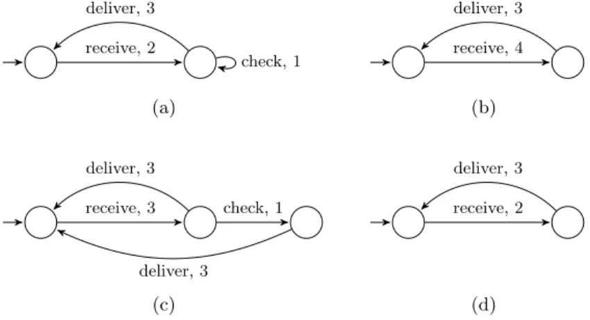
Fig. 5: Specification of a simple email system, similar to Fig. 1, but extended by integer intervals modeling time units for performing the corresponding actions.
quantitative aspects [3, 19]. With these applications in mind, it is necessary not
only to be able to specify quantitative aspects of systems, but also to formalize successive refinement of quantities. To illustrate this extension, consider again the modal transition system of Fig. 1, but this time with quantities, see Fig. 5: Every transition label is extended by integer intervals modeling upper and lower bounds on time required for performing the corresponding actions. For instance, the reception of a new email (action receive) must take between one and three time units, the checking of the email (action check ) is allowed to take up to five time units.
In this quantitative setting, there is a problem with using a Boolean notion of refinement as is done in the preceding section: If one only can decide whether or not an implementation refines a specification, then the quantitative aspects get lost in the refinement process. As an example, consider the email system implementations in Fig. 6. Implementation (a) does not refine the specification, as there is an error in the discrete structure of actions: after receiving an email, the system can check it indefinitely without ever delivering it. Also implementations (b) and (c) do not refine the specification: (b) takes too long to receive email, (c) does not deliver email fast enough after checking it. Implementation (d) on the other hand is a perfect refinement of the specification.
Intuitively however, implementations (b) and (c) conform much better to the specification than implementation (a) in Fig. 6: there are no discrepancies in the discrete structure, only the weights are off by 1. Additionally, the quantitative error in implementation (c) occurs later than the one in (b). Hence one may want to say that implementation (d) is in perfect refinement of the specification, (c) is slightly off, (b) is a bit more problematic, whereas implementation (a) is completely unacceptable. A Boolean notion of refinement does not allow to make such distinctions between different negative answers.
To sum up, a Boolean notion of refinement is too fragile for quantitative formalisms. Minor and major modifications in the implementation cannot be distinguished, as both of them may reverse the Boolean answer. As observed
e.g. in [9], this view is obsolete; engineers need quantitative notions on how
modified implementations differ. The introduction of such a quantitative notion of refinement, and its consequences for the specification theory, are the subject of this section, which is based on the papers [1, 2].
receive, 2 deliver, 3 check, 1 (a) receive, 4 deliver, 3 (b) receive, 3 deliver, 3 check, 1 deliver, 3 (c) receive, 2 deliver, 3 (d)
Fig. 6: Four implementations of the simple email system in Fig. 5.
Depending on the precise application of our quantitative formalism, there are a few choices which one has to make. One such choice is the precise definition of quantitative refinement, as the way quantitative discrepancies between specifica-tions is measured e.g. depends on whether differences accumulate over time or the interest more lies in the maximal individual differences. Another choice is how to combine quantities during structural composition: when modeling e.g. energy consumption, they should be added; when modeling timing constraints, some form of conjunction should be used.
To facilitate quantitative reasoning on specifications and implementations, we introduce a real-valued distance between specifications such that perfect refinement corresponds to distance 0, small quantitative discrepancies give rise to small distances, and differences in the discrete control structure correspond to distance ∞. For the examples in Figs. 5 and 6, we will deduce the following chain of decreasing distances:
∞ = d(I1, S) > d(I2, S) > d(I3, S) > d(I4, S) = 0
3.1 Weighted modal transition systems
Let Σ be a set of labels with a preorder ⊑ ⊆ Σ ×Σ, and denote by Σ∞= Σ∗∪Σω
the set of finite and infinite traces over Σ. len(σ), for σ ∈ Σ∞, denotes the length
(finite or infinite) of a trace σ. Let ε ∈ Σ∞ denote the empty trace, and for
a ∈ Σ, σ ∈ Σ∞, denote by a.σ their concatenation.
A weighted modal transition system (WMTS) is a tuple S = (S, s0
, 99K, −→) consisting of a set S of states, an initial state s0 ∈ S, and must- and
may-transitions −→, 99K ⊆ S × Σ × S for which it holds that for all s−→ sa ′ there is
Intuitively, a may-transition s99K t specifies that an implementation I of Sb is permitted to have a corresponding transition i−→ j, for any a ⊑ b, whereas aa must-transition s−→ t postulates that I is required to implement at least oneb corresponding transition i−→ j for some a ⊑ b. We will make this precise below.a
An WMTS S = (S, s0
, 99K, −→) is an implementation if −→ = 99K. Hence in an implementation, all optional behavior has been resolved.
Definition 3. A modal refinement of WMTS S1 = (S1, s01, 99K1, −→1), S2 =
(S2, s02, 99K2, −→2) is a relation R ⊆ S1× S2 such that for any (s1, s2) ∈ R,
– whenever s1 a1
99K1t1, then also s2 a2
99K2t2 for some a1⊑ a2 and (t1, t2) ∈ R,
– whenever s2−→a2
2t2, then also s1 a1
−→1t1 for some a1⊑ a2 and (t1, t2) ∈ R.
Thus any behavior which is permitted in S1is also permitted in S2, and any
behavior required in S2 is also required in S1. We write S1≤m S2 if there is a
modal refinement R ⊆ S1× S2with (s01, s 0 2) ∈ R.
The implementation semantics of a WMTS S is the set JKS = {I ≤m
S | I implementation}, and we write S1 ≤t S1 if JS1K ⊆ JS2K, saying that S1 thoroughly refines S2. It follows by transitivity of ≤m that S1 ≤m S2 implies
S1≤tS2, hence modal refinement is a syntactic over-approximation of thorough
refinement.
3.2 Distances
Recall that a hemimetric on a set X is a function d : X × X →❘≥0∪ {∞} which
satisfies d(x, x) = 0 and d(x, y) + d(y, z) ≥ d(x, z) (the triangle inequality) for all x, y, z ∈ X. Note that our hemimetrics are extended in that they can take the value ∞.
We will need to generalize hemimetrics to codomains other than❘≥0∪ {∞}.
For a partially ordered monoid (▲, ⊑, ⊕, ✵), an ▲-hemimetric on X is a function d : X × X →▲ which satisfies d(x, x) = ✵ and d(x, y) ⊕ d(y, z) ⊒ d(x, z) for all x, y, z ∈ X.
Definition 4. A trace distance is a hemimetric td : Σ∞× Σ∞→❘
≥0∪ {∞} for which td(a, b) = 0 for all a, b ∈ Σ with a ⊑ b and td(σ, τ ) = ∞ whenever
len(σ) 6= len(τ ).
For any set M , let ▲M = (❘≥0∪ {∞})M the set of functions from M to
the extended non-negative real line. Then▲M is a complete lattice with partial order ⊑ ⊆▲M × ▲M given by α ⊑ β if and only if α(x) ≤ β(x) for all x ∈ M, and with an addition ⊕ given by (α ⊕ β)(x) = α(x) + β(x). The bottom element of ▲M is also the zero of ⊕ and given by ⊥(x) = 0, and the top element is ⊤(x) = ∞.
Definition 5. A recursive specification of a trace distance td consists of
– an▲M-hemimetric td▲M : Σ∞× Σ∞→▲M which satisfies td = eval◦td▲M and td▲M(a, b) = ⊥ for all a, b ∈ Σ with a ⊑ b, and
– a function F : Σ × Σ ×▲M → ▲M.
F must be monotone in the third coordinate and satisfy, for all a, b ∈ Σ and σ, τ ∈ Σ∞, that td▲M(a.σ, b.τ ) = F (a, b, td▲M(σ, τ )).
Note that the definition implies that for all a, b ∈ Σ, td▲M(a, b) =
td▲M(a.ε, b.ε) = F (a, b, td▲M(ε, ε)) = F (a, b, ⊥). Hence also F (a, a, ⊥) =
td▲M(a, a) = ⊥ for all a ∈ Σ.
We have shown in [2, 10, 12] that all commonly used trace distances obey a recursive characterization as above. The point-wise distance from [8], for example, has ▲ = ❘≥0∪ {∞}, eval = id and d▲Mm (a.σ, b.τ ) = max(d(a, b), d▲Mm (σ, τ )),
where d : Σ × Σ → ❘≥0∪ {∞} is a hemimetric on labels. The limit-average
distance used in e.g. [7] has▲ = (❘≥0∪ {∞})◆, the complete lattice of functions
◆ → ❘≥0∪ {∞}, eval(α) = lim infj∈◆α(j) and d▲Mm (a.σ, b.τ )(j) = 1
j+1d(a, b) + j
j+1d▲Mm (σ, τ ).
For the rest of this section, we fix a recursively specified trace distance. A WMTS (S, s0
, 99K, −→) is deterministic if it holds for all s ∈ S, s a1 99K s1, s
a2 99K s2
for which there is a ∈ Σ with td▲M(a, a1) 6= ⊤ and td▲M(a, a2) 6= ⊤ that a1= a2
and s1= s2.
Definition 6. The lifted modal refinement distance d▲Mm : S1× S2→▲ between the states of WMTS S1= (S1, s01, 99K1, −→1), S2= (S2, s02, 99K2, −→2) is defined to be the least fixed point to the equations
d▲Mm (s1, s2) = max sup s199Ka11t1 inf s299Ka22t2 F (a1, a2, d▲Mm (t1, t2)), sup s2−→a22t2 inf s1−→a11t1 F (a1, a2, d▲Mm (t1, t2)). We let d▲Mm (S1, S2) = d▲Mm (s 0 1, s 0
2). The modal refinement distance is dm =
eval◦ d▲Mm , and we write S1≤ ε
mS2, for ε ∈❘≥0∪ {∞}, if d▲Mm (S1, S2) ≤ ε.
Proposition 1. The modal refinement distance is a well-defined hemimetric, and S1≤mS2 implies S1≤0mS2.
The thorough refinement distance between WMTS S1, S2is
dt(S1, S2) = sup I1∈JS1K
inf
I2∈JS2K
dm(I1, I2),
and we write S1≤εt S2, for ε ∈❘≥0∪ {∞}, if dt(S1, S2) ≤ ε. As for the modal
distance, dt is a hemimetric, and S1≤t S2implies S1≤0t S2.
Theorem 1. For all WMTS S1, S2, dt(S1, S2) ≤ dm(S1, S2). If S2 is determin-istic, then dt(S1, S2) = dm(S1, S2).
3.3 Conjunction
Let ? : Σ ×Σ ֒→ Σ be a commutative partial label conjunction operator for which it holds, for all b1, b2 ∈ Σ, that there is a ∈ Σ for which both td▲M(a, b1) 6= ⊤
and td▲M(a, b2) 6= ⊤ iff there exists c ∈ Σ for which both b1? c and b2? c are
defined. This is to relate determinism (left-hand side of the above) to a similar property for label conjunction which is needed in the proof of Theorem 2.
Additionally, we assume that ? is greatest lower bound on labels, i.e.
– for all a, b ∈ Σ with a ? b defined, a ? b ⊑ a and a ? b ⊑ b;
– for all a, b, c ∈ Σ with a ⊑ b and a ⊑ c, b ? c is defined and a ⊑ b ? c.
In the definition below, we denote by ρB(S) the pruning of a WMTS S =
(S, s0
, 99K, −→) with respect to the states in a (“bad”) subset B ⊆ S, which is obtained as follows: Define a must-predecessor operator pre : 2S → 2S by
pre(S′) = {s ∈ S | ∃a ∈ Σ, s′ ∈ S′ : s −→ sa ′} and let pre∗ be the reflexive,
transitive closure of pre. Then ρB(S) is defined if s0∈ pre/ ∗(B), and in that case,
ρB(S) = (Sρ, s0, 99Kρ, −→ρ) with Sρ= S \ pre∗(B), 99Kρ= 99K ∩ (Sρ× Σ × Sρ),
and −→ρ= −→ ∩ (Sρ× Σ × Sρ).
Definition 7. The conjunction of two WMTS S1= (S1, s01, 99K1, −→1), S2=
(S2, s02, 99K2, −→2) is the WMTS S1∧ S2= ρB(S1× S2, (s01, s 0
2), 99K, −→) given as follows (if it exists):
s1 a 1 −→1t1 s2 a 2 99K2t2 a1?a2 defined (s1, s2) a 1?a2 −→ (t1, t2) s1 a 1 99K1t1 s2 a 2 −→2t2 a1?a2 defined (s1, s2) a 1?a2 −→ (t1, t2) s1 a 1 99K1t1 s2 a 2 99K2t2 a1?a2 defined (s1, s2) a 1?a2 99K (t1, t2) s1 a 1 −→1t1 ∀s2 a 2 99K2t2: a1?a2 undef. (s1, s2) ∈ B s2 a 2 −→2t2 ∀s1 a 1 99K1t1: a1?a2 undef. (s1, s2) ∈ B
Note that conjunction of WMTS may give inconsistent states which need to be pruned away after. As seen in the last two SOS rules above, this is the case when one WMTS specifies a must-transition which the other WMTS cannot synchronize with. Here, the demand on implementations of the conjunction would be that they simultaneously must and cannot have a transition, which of course is unsatisfiable.
Theorem 2. Let S1, S2, S3 be WMTS.
– If S1∧ S2 is defined, then S1∧ S2≤mS1 and S1∧ S2≤mS2.
– If S1≤mS2, S1≤mS3, and S2or S3is deterministic, then S2∧ S3is defined and S1≤mS2∧ S2.
3.4 Structural composition
Let ȅ : Σ × Σ ֒→ Σ be a commutative partial label composition operator which specifies which labels can synchronize. Again we need to relate determinism to an analogous property for label composition, hence we require that it holds, for all b1, b2∈ Σ, that there is a ∈ Σ for which both d(a, b1) 6= ⊤▲ and d(a, b2) 6= ⊤▲
iff there exists c ∈ Σ for which both b1ȅ c and b2ȅ c are defined.
Additionally, we assume that there exists a function P :▲ × ▲ → ▲ which allows us to infer bounds on distances on synchronized labels. We assume that P is monotone in both coordinates, has P (⊥▲, ⊥▲) = ⊥▲, P (α, ⊤▲) = P (⊤▲, α) =
⊤▲ for all α ∈▲, and that
F (a1ȅ a2, b1ȅ b2, P (α1, α2)) ⊑▲P (F (a1, b1, α1), F (a2, b2, α2)) (1)
for all a1, b1, a2, b2∈ Σ and α1, α2∈▲ for which a1ȅ a2 and b1ȅ b2 are defined.
Hence d(a1ȅ a2, b1ȅ b2) ⊑ P (d(a1, b1), d(a2, b2)) for all such a1, b1, a2, b2∈ Σ.
Intuitively, P gives a uniform bound on label composition: distances be-tween composed labels can be bounded above using P and the individual labels’ distances, and (1) ensures that this bound holds recursively.
Definition 8. The structural composition of two WMTS S1= (S1,s01,99K1,−→1),
S2= (S2, s02, 99K2, −→2) is the WMTS S1kS2= (S1× S2, (s10, s 2
0), 99K, −→) with transitions defined as follows:
s1 a1 99K1t1 s2 a2 99K2t2 a1ȅ a2 def. (s1, s2) a1ȅa2 99K (t1, t2) s1 a1 −→1t1 s2 a2 −→2t2 a1ȅ a2 def. (s1, s2) a−→ (t1ȅa2 1, t2)
The next theorem shows that structural composition supports quantitative
independent implementability: the distance between structural compositions can
bounded above using P and the distances between the individual components. Theorem 3. For all WMTS S1, T1, S2, T2 with dm(S1kS2, T1kT2) 6= ⊤▲, we have dm(S1kS2, T1kT2) ⊑▲ P (dm(S1, T1), dm(S2, T2)).
References
1. Sebastian S. Bauer, Uli Fahrenberg, Line Juhl, Kim G. Larsen, Axel Legay, and Claus Thrane. Quantitative refinement for weighted modal transition systems. In MFCS, volume 6907 of LNCS, pages 60–71. Springer, 2011.
2. Sebastian S. Bauer, Uli Fahrenberg, Axel Legay, and Claus Thrane. General quantitative specification theories with modalities. In CSR, volume 7353 of LNCS, pages 18–30. Springer, 2012.
3. Sebastian S. Bauer, Line Juhl, Kim G. Larsen, Axel Legay, and Jiří Srba. Extending modal transition systems with structured labels. Mathematical Structures in Computer Science, 22(4):581–617, 2012.
4. Nikola Beneš, Jan Křetínský, Kim G. Larsen, Mikael H. Møller, and Jiří Srba. Parametric modal transition systems. In ATVA, volume 6996 of LNCS, pages 275–289. Springer, 2011.
5. Nikola Beneš and Jan Křetínský. Process algebra for modal transition systemses. In MEMICS, volume 16 of OASICS, pages 9–18. Schloss Dagstuhl - Leibniz-Zentrum fuer Informatik, Germany, 2010.
6. Gérard Boudol and Kim G. Larsen. Graphical versus logical specifications. In CAAP, volume 431 of LNCS, pages 57–71. Springer, 1990.
7. Pavol Černý, Thomas A. Henzinger, and Arjun Radhakrishna. Simulation distances. Theor. Comput. Sci., 413(1):21–35, 2012.
8. Luca de Alfaro, Marco Faella, Thomas A. Henzinger, Rupak Majumdar, and Mariëlle Stoelinga. Model checking discounted temporal properties. Theor. Comput. Sci., 345(1):139–170, 2005.
9. Luca de Alfaro, Marco Faella, and Mariëlle Stoelinga. Linear and branching system metrics. IEEE Trans. Software Eng., 35(2):258–273, 2009.
10. Uli Fahrenberg, Axel Legay, and Claus Thrane. The quantitative linear-time– branching-time spectrum. In FSTTCS, volume 13 of LIPIcs, pages 103–114. Schloss Dagstuhl - Leibniz-Zentrum fuer Informatik, 2011.
11. Uli Fahrenberg, Axel Legay, and Louis-Marie Traonouez. Specification theories for probabilistic and real-time systems. In From Programs to Systems – The Systems Perspective in Computing, volume 8415 of LNCS. Springer, 2014. In this volume. 12. Uli Fahrenberg, Claus R. Thrane, and Kim G. Larsen. Distances for weighted
transition systems: Games and properties. In QAPL, volume 57 of Electr. Proc. Theor. Comput. Sci., pages 134–147, 2011.
13. Harald Fecher and Heiko Schmidt. Comparing disjunctive modal transition systems with an one-selecting variant. J. Logic Alg. Program., 77(1-2):20–39, 2008. 14. Patrice Godefroid, Michael Huth, and Radha Jagadeesan. Abstraction-based model
checking using modal transition systems. In CONCUR, volume 2154 of LNCS, pages 426–440. Springer, 2001.
15. Susanne Graf and Joseph Sifakis. A logic for the description of non-deterministic programs and their properties. Inf. Control, 68(1-3):254–270, 1986.
16. Alexander Gruler, Martin Leucker, and Kathrin D. Scheidemann. Modeling and model checking software product lines. In FMOODS, volume 5051 of LNCS, pages 113–131. Springer, 2008.
17. Sören Holmström. A refinement calculus for specifications in Hennessy-Milner logic with recursion. Formal Asp. Comput., 1(3):242–272, 1989.
18. Michael Huth, Radha Jagadeesan, and David A. Schmidt. Modal transition systems: A foundation for three-valued program analysis. In ESOP, volume 2028 of LNCS, pages 155–169. Springer, 2001.
19. Line Juhl, Kim G. Larsen, and Jiří Srba. Modal transition systems with weight intervals. J. Log. Algebr. Program., 81(4):408–421, 2012.
20. Kim G. Larsen. A context dependent equivalence between processes. Theor. Comput. Sci., 49:184–215, 1987.
21. Kim G. Larsen. Modal specifications. In Automatic Verification Methods for Finite State Systems, volume 407 of LNCS, pages 232–246. Springer, 1989.
22. Kim G. Larsen, Ulrik Nyman, and Andrzej Wąsowski. On modal refinement and consistency. In CONCUR, volume 4703 of LNCS, pages 105–119. Springer, 2007. 23. Kim G. Larsen and Bent Thomsen. A modal process logic. In LICS, pages 203–210.
IEEE Computer Society, 1988.
24. Kim G. Larsen and Liu Xinxin. Equation solving using modal transition systems. In LICS, pages 108–117. IEEE Computer Society, 1990.
25. Radu Mardare and Alberto Policriti. A complete axiomatic system for a process-based spatial logic. In MFCS, volume 5162 of LNCS, pages 491–502. Springer, 2008.
26. Sebastian Nanz, Flemming Nielson, and Hanne Riis Nielson. Modal abstractions of concurrent behaviour. In SAS, volume 5079 of LNCS, pages 159–173. Springer, 2008.
27. Jean-Baptiste Raclet, Eric Badouel, Albert Benveniste, Benoît Caillaud, and Roberto Passerone. Why are modalities good for interface theories? In ACSD, pages 119–127. IEEE, 2009.
28. Sebastián Uchitel and Marsha Chechik. Merging partial behavioural models. In FSE, pages 43–52. ACM, 2004.