HAL Id: inria-00352091
https://hal.inria.fr/inria-00352091
Submitted on 12 Jan 2009
HAL is a multi-disciplinary open access
archive for the deposit and dissemination of
sci-entific research documents, whether they are
pub-lished or not. The documents may come from
L’archive ouverte pluridisciplinaire HAL, est
destinée au dépôt et à la diffusion de documents
scientifiques de niveau recherche, publiés ou non,
émanant des établissements d’enseignement et de
Motion-based obstacle detection and tracking for car
driving assistance
G. Lefaix, E. Marchand, Patrick Bouthemy
To cite this version:
G. Lefaix, E. Marchand, Patrick Bouthemy. Motion-based obstacle detection and tracking for car
driving assistance. IAPR Int. Conf. on Pattern Recognition, ICPR’02, 2002, Quebec, Canada,
Canada. pp.74-77. �inria-00352091�
IAPR Int. Conf. on Pattern Recognition, ICPR’2002 volume 4, pages 74–77, Qu´ebec, Canada, August 2002
Motion-based Obstacle Detection and Tracking for Car Driving Assistance
Gildas Lefaix, ´
Eric Marchand, Patrick Bouthemy
I
RISA- I
NRIARennes
Campus de Beaulieu, 35042 Rennes Cedex, France
Abstract
This paper is concerned with the detection and track-ing of obstacles from a camera mounted on a vehicle with a view to driver assistance. To achieve this goal, we have designed a technique entirely based on image motion analy-sis. We perform the robust estimation of the dominant image motion assumed to be due to the camera motion. Then by considering the outliers to the estimated dominant motion, we can straightforwardly detect obstacles in order to assist car driving. We have added to the detection step a tracking module that also relies on a motion consistency criterion. Time-to-collision is then computed for each validated ob-stacle. We have thus developed an application-oriented so-lution which has proven accurate, reliable and efficient as demonstrated by experiments on numerous real situations.
1. Introduction
This paper is concerned with the detection and tracking of obstacles from a camera mounted on a vehicle with a view to driver assistance. This work is part of the Carsense European project [3]. The goal of this project is to develop a sensor system to deliver information on the car environment at low speed to assist low-speed driving. The combination of several sensors should improve object detection. Indeed various sensors are considered in the Carsense project: short and long range radar, laser sensor, and video cameras. Each sensor is nevertheless supposed to be independent. Extract-ed information from the different sensors will be fusExtract-ed at a further step in order to reduce false alarm rate and to handle possible missing data.
We are concerned with the image-based obstacle detec-tion task. The aim is to detect obstacles located at less than 50 meters in front of the cat. Such an obstacle could be a vehicle (car, truck), a motor-bike, a bicycle or a pedestrian crossing the car trajectory. The goal is to develop fast and efficient vision algorithms to detect obstacles on the road and to reconstruct their trajectories wrt. the camera, for all static or moving detected obstacle. To achieve this goal, we have designed a technique based on motion analysis as
pro-posed in [1, 2, 7, 4]. We first compute the dominant image motion assumed to be due to the car motion [4, 6]. It is rep-resented by a 2D quadratic motion model which correspond to the projection of the rigid motion of a planar surface (here, the road). It is estimated by a robust multi-resolution technique [6]. Detection of obstacles can then be performed by considering that their apparent image motion is not con-forming the computed dominant motion. Once detected the objects (or obstacles) are tracked using a motion-based pro-cess. The trajectories and the time-to-collision associated to each obstacle are then be computed and are supplied as input of the data-fusion module. In, e.g., [2] the expect-ed image motion was computexpect-ed using the vehicle odometry and was not estimated using image information. The main advantage of the presented algorithm is that it does not con-sider any information but the images acquired by the camera and that it allows fast computation on standard hardware.
The reminder of the paper is organized as follows. In Section 2 we outline the dominant image motion estima-tion method. Secestima-tion 3 then describes the detecestima-tion and tracking of the obstacles and the computation of the time-to-collision. In Section 4, we report experimental results related to our application.
2. Dominant motion estimation
The estimation of the 2D parametric motion model ac-counting the dominant image motion is achieved with a ro-bust, multi-resolution, and incremental estimation method exploiting only the spatio-temporal derivatives of the inten-sity function [6].
Quadratic motion models. Since the near car environ-ment free of obstacles is formed by the road which can be considered as a planar surface, the image dominant mo-tion due to the car momo-tion can be exactly represented by a 2D quadratic motion model involving eight free parame-ters. Let us denoteΘ = (a0, a1, a2, a3, a4, a5, a6, a7), the
velocity vector WΘ(P ) at pixel P = (u, v) corresponding
WΘ(P ) = h a0 a1 i + h a2 a3 a4 a5 i h u v i + h a6 a7 0 0 a6 a7 i" u2 uv v2 # (1)
Dominant image motion estimation To estimate the dominant image motion between two successive imagesIt
andIt+1, we use the gradient-based multiresolution robust
estimation method described in [6]. To ensure robustness to the presence of independent motion, we minimize a M-estimator criterion with a hard-redescending function. The constraint is given by the usual assumption of brightness constancy of a projected surface element over its 2D trajec-tory. Thus, the motion model estimation is defined as:
b Θ = argmin Θ E(Θ) = argminΘ X P∈R(t) ρ (DFDΘ(P )) (2) with DFDΘ(P ) = It+1(P + WΘ(P )) − It(P ) . (3)
ρ(x) is the Tukey’s biweight function. The estimation sup-port R(t) can be the whole image. In practice, it will be restricted to a specific area of the image. The minimiza-tion is embedded in a multi-resoluminimiza-tion framework and fol-lows an incremental scheme. At each incremental stepk, we can write: Θ = bΘk + ∆Θk, where bΘk is the
curren-t escurren-timacurren-te of curren-the paramecurren-ter veccurren-torΘ. A linearization of DFDΘ(P ) around bΘk is performed, leading to a residual
quantityr∆Θk(P ) linear with respect to ∆Θk:
r∆Θ
k(P ) = ∇It(P + WbΘk(P )).W∆Θk(P )
+It+1(P + W
b
Θk(P )) − It(P )
where ∇It(P ) denotes the spatial gradient of the intensity
function. Then, we consider the minimization of the expres-sion given by
Ea(∆Θk) =
X
P
ρ (r∆Θk(P )) . (4)
This function is minimized using an Iterative-Reweighted-Least-Squares procedure. It means that the expression (4) is replaced by: Ea(∆Θk) = 1 2 X P ω(P )r∆Θk(P ) 2, (5)
and that we alternatively estimates ∆Θk and update the
weightsω(P ) (whose initial value are 1).
This method allows us to get a robust and accurate es-timation of the dominant image motion (i.e., background apparent motion) between two images.
3. Obstacles detection and tracking
3.1. Obstacles detection
The previous step supplies two sets of information:
• the motion parameters bΘ corresponding to the domi-nant motion;
• the mapIωof the weightsω(P ) used in (5) which
ac-count for the fact that pixelP is conforming or not to the computed dominant motion.
The mapsIwwill be used to detect the obstacles from the
image sequences. Let us recall that the considered quadrat-ic motion model is supposed to correspond to the apparent motion of the road surface. Therefore, each pixel that is not conform to this estimated motion can be considered as be-longing to an obstacle, either static or moving (or to another part of the scene, if it does not lie on the road).
The outliers map Iω is thresholded and mathematical
morphology operators are applied in order to suppress noise. Pixels are then merged into group of pixels accord-ing to various criteria (distance or motion-based criterion). Concerning the distance criterion, two pixels or regions (group of pixels) are merged if they are connex or if the distance between these two groups is below a given thresh-old. Concerning the motion similarity criterion, two regions RiandRj are merged in a single regionRf if the motion
within regionRiis consistent with the motion inRf and if
the motion inRjis consistent with the motion inRf. It is
defined as:
C = Cif + Cjf (6)
whereCkf reflects the motion similarity between regions
Rk|k=i,jandRf: Ckf = 1 Card (Rk) X P∈Rk duΘbk−du b Θf + dvbΘk−dv b Θf (7) where dΘ = (duΘ, d v
Θ) denotes the displacement of pixel
P = (u, v) according to the motion model Θ, and bΘk
des-ignates the parameters of the motion model estimated with-in regionRkusing the same method as the one described in
Section 2.Card(R) is the number of pixels in region R.
3.2. Obstacle tracking
We then obtain for each obstacle (or, more precisely, for each area in the image that is not conforming to the domi-nant motion) a bounding area. In order to improve the ef-ficiency of this approach and to limit the number of false alarms, these areas are tracked over successive frames.
A comparison between obstacle areas detected in two successive images is then necessary. Two tests both based on motion similarity have been investigated. The first one exploits the criterion defined in (6). The second, which as-sumes that the two regions overlap, and evaluates the mo-tion consistency in the intersecmo-tion of the two regions. It
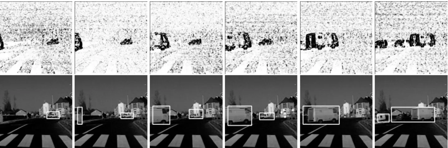
Figure 1. Obstacle detection from a motionless vehicle. The first and third rows display the outliers maps, the second and fourth rows contains the detected obstacles (see text for details)
can be expressed as follows: Cij= 1 Card (Ri∩Rj) · X P∈Ri∩Rj dubΘj −du b Θi + dvbΘj −dv b Θi (8) This short term temporal tracking allow us to suppress false detections that could arise in a one-frame analysis. At this step we have a set of obstacle areas validated in the current frame and specified by their bounding rectangular boxes, and their position in the previous frame.
3.3. Time-To-Collision
For each detected obstacle, we can now compute the time-to-collision with the camera using the motion model computed in the bounding area. The time-to-collision is given by: τc(u, v) = −TZ
Z, whereZ is the depth of the
obstacle andTZthe relative object velocity along the
cam-era view axis. Assuming a planar object surface (at least a “shallow” object), we can writeZ = Z0+ γ1X + γ2Y and
τccan be rewritten as:
τc(u, v) = − Z0 TZ 1 (1 − γ1x − γ2y) (9) x and y are obtained assuming the knowledge of the camera intrinsic parameters:x = (u − u0)/pxandy = (v − v0)/py
((u0, v0) are the coordinates of the camera principal point
whilepxandpyreflects the pixel size). γ1,γ2andZ0/TZ
can be computed from the affine parameters of the motion model[a1, a2, a3, a4, a5, a6] defined in (1) computed
with-in the boundwith-ing area for each obstacle at each with-instant. the relation have been derived in [5].
4. Results
The proposed method has been implemented on a PC running Linux. Each frame is processed in 0.4 s for
512×512 images and in 0.1 s for 256×256 images. We have tested our approach on numerous image sequences acquired in different contexts. We only report here four representa-tive experiments.
In the first sequence, the car with the camera is motion-less. Several vehicles are crossing the road in front of the camera (see Figure 1). Although this example is simple s-ince it involves a static camera, it allows to validate the ob-stacles detection and tracking modules. The obob-stacles are successfully detected and tracked over the image sequence. In the fourth image of Figure 1 although the van and the car are close to each another they are correctly considered as two different vehicles since their motions are not homo-geneous (according to the criterion of relation (6)). After they cross each other, they are again recovered (see the last image of Figure 1). In the same image the black car closely following the van is detected as a part of the same object. Indeed, it has the same motion features as the van.
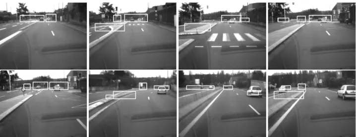
In the second experiment, we consider a mobile camera following a van in an urban environment (see Figure 2). The van and the other vehicle (last image) are correctly detected and tracked over the image sequence. The time-to-collision was computed as described in Sub-section 3.3. Let us stress that the time-to-collision values plotted in Figure 2 have not been filtered over time (which could be easily implement-ed and could smooth the obtainimplement-ed plot). It proves that the time-to-collision computation is consistent. In experiments reported in Figure 3 and Figure 4 the car is moving within a more complex environment: a highway and a road. For efficiency concern, the dominant motion is not estimated in the whole image but only in an area delineated on the first image of Figure 3 (i.e., between the two dashed lines). Ob-stacles are again correctly detected and tracked even if a few false alarms may appear in some frames. Let us point out that objects lying close to the road as well as some
road-Figure 4. Detection of multiple (moving and static) obstacles in a road environment. 40 60 80 100 120 140 160 180 200 220 240 0 10 20 30 40 50 60 70 time to collision
Figure 2. Obstacle detection and tracking in a urban en-vironment. Plot corresponding to the computed time-to-collision values over time for the detected obstacle (white van).
Figure 3. Obstacle detection and tracking in a highway environment
signs are correctly detected.
5. Conclusion
We have presented an accurate and efficient method based on the robust estimation of the dominant image mo-tion to detect obstacles in order to assist car driving. We have added to the detection step a tracking module that also relies on a motion consistency criterion. Time-to-collision is then computed for each validated obstacle. Our goal was to proposed an algorithm that does not consider any other input but the images acquired by the camera. Furthermore we seek fast and robust computation on low-cost standard hardware. With respect to the considered application that is assistance at low-speed driving, quite satisfactory results on various real image sequences have validated our approach.
References
[1] N. Ancona, T. Poggio. Optical flow from 1d correlation: Application to a simple time-to-crash detector. IJCV, 14(2):131–146, 1995. [2] W. Enkelmann. Obstacle detection by evaluation of optical flow field
from image sequences. Image an Vision Computing, 9:160–168, 1991. [3] J. Langheim. Sensing of car environment at low speed driving. In 7th
World Congress on Intelligent Transport Systems, Torino, , Oct. 2000.
[4] W. Kr ¨uger. Robust real-time ground plane motion compensation from a moving vehicle. Machine Vision and App., 11(4):203–212, 1999. [5] F. Meyer, P. Bouthemy. Estimation of time-to-collision maps from
first order motion models and normal flows. In ICPR92, pages 78–82, 1992.
[6] J.-M. Odobez, P. Bouthemy. Robust multiresolution estimation of parametric motion models. Journal of Visual Communication and
Im-age Representation, 6(4):348–365, December 1995.
[7] J. Santos-Victor, G. Sandini. Uncalibrated obstacle detection using normal flow. Machine Vision and Application, 9(3):130–137, 1996.