HAL Id: hal-01144152
https://hal-imt.archives-ouvertes.fr/hal-01144152
Submitted on 14 Oct 2019
HAL is a multi-disciplinary open access
archive for the deposit and dissemination of
sci-entific research documents, whether they are
pub-lished or not. The documents may come from
teaching and research institutions in France or
abroad, or from public or private research centers.
L’archive ouverte pluridisciplinaire HAL, est
destinée au dépôt et à la diffusion de documents
scientifiques de niveau recherche, publiés ou non,
émanant des établissements d’enseignement et de
recherche français ou étrangers, des laboratoires
publics ou privés.
Impromptu Deployment of Wireless Relay Networks:
Experiences Along a Forest Trail
Arpan Chattopadhyay, Avishek Ghosh, Akhila S. Rao, Bharat Dwivedi,
S.V.R. Anand, Marceau Coupechoux, Anurag Kumar
To cite this version:
Arpan Chattopadhyay, Avishek Ghosh, Akhila S. Rao, Bharat Dwivedi, S.V.R. Anand, et al..
Im-promptu Deployment of Wireless Relay Networks: Experiences Along a Forest Trail. IEEE
Interna-tional Conference on Mobile Ad hoc and Sensor Systems (MASS), Oct 2014, Philadelphia, United
States. pp.1-5. �hal-01144152�
Impromptu Deployment of Wireless Relay
Networks: Experiences Along a Forest Trail
Arpan Chattopadhyay, Avishek Ghosh, Akhila S. Rao, Bharat Dwivedi,
S.V.R. Anand, Marceau Coupechoux, and Anurag Kumar
Abstract—We are motivated by the problem of impromptu oras-you-go deployment of wireless sensor networks. As an application example, a person, starting from a sink node, walks along a forest trail, makes link quality measurements (with the previously placed nodes) at equally spaced locations, and deploys relays at some of these locations, so as to connect a sensor placed at some a priori unknown point on the trail with the sink node. In this paper, we report our experimental experiences with some as-you-go deployment algorithms. Two algorithms are based on Markov decision process (MDP) formulations; these require a radio propagation model. We also study purely measurement based strategies: one heuristic that is motivated by our MDP formulations, one asymptotically optimal learning algorithm, and one inspired by a popular heuristic. We extract a statistical model of the propagation along a forest trail from raw measurement data, implement the algorithms experimentally in the forest, and compare them. The results provide useful insights regarding the choice of the deployment algorithm and its parameters, and also demonstrate the necessity of a proper theoretical formulation.
I. INTRODUCTION
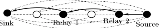
Our work in this paper is motivated by the need for as-you-go deployment of wireless relay networks over large terrains, such as forest trails, where planned deployment would be time-consuming and difficult. As-you-go deployment is the only choice when the network is temporary and needs to be quickly redeployed, or when the deployment needs to be stealthy. In this paper, we are concerned with an experimental study of the problem of deploying wireless relay nodes as a deployment agent walks along a forest trail, in order to connect a sink at the start of the trail to a sensor that would need to be deployed at an a priori unknown point. The sensor could be an animal activity detector based on passive infra-red (PIR) sensors, or even a “camera trap,” that has to be placed near a watering hole that is known to exist somewhere just off the trail. Figure 1 depicts the abstraction of the problem along a line. The sink has a “backhaul” communication link to a control center. In planned deployment, we need to place relay nodes at all potential locations (see Figure 1 for a simple depiction) and
Arpan Chattopadhyay, Avishek Ghosh, Bharat Dwivedi, S.V.R. Anand, and Anurag Kumar are with the Department of ECE, Indian Institute of Science, Bangalore, India; email: arpanc.ju@gmail.com, {avishek, bharat, anand, anurag}@ece.iisc.ernet.in. Akhila S. Rao is with KTH, Royal In-stitute of Technology, Stockholm, Sweden; email: akhila@kth.se. Marceau Coupechoux is with Telecom ParisTech and CNRS LTCI, Dept. Infor-matique et Reseaux, 23, avenue d’Italie, 75013 Paris, France; email: marceau.coupechoux@telecom-paristech.fr.
This work was supported by (i) the Department of Electronics and Infor-mation Technology (India) and the National Science Foundation (USA) via an Indo-US collaborative project titled Wireless Sensor Networks for Protecting Wildlife and Humans, and (ii) the J.C. Bose National Fellowship (of the Govt. of India).
This paper is a shortened version of our detailed technical report [1].
Sink
Relay1
Relay2
Sour e
Fig. 1. Two wireless relays (filled dots) deployed along a line to connect a
source to a sink by a multihop path. The unfilled dots show other potential relay placement locations, the thin dashed lines indicate all the potential links between the potential placement locations, and the solid lines with arrowheads indicate the links actually used in the deployed network.
measure the qualities of all possible (solid and dotted) links (between all pairs of potential locations; see Figure 1) in order to decide where to place the relays. This would yield a global optimal solution, but with huge time and effort. With as-you-go deployment, the next relay placement locations depend on the radio link qualities to the previously placed nodes; link qualities and the location of the sensor node are discovered as the agent walks along the trail. Such an approach requires fewer measurements compared to planned deployment, but is suboptimal. In this paper, we report the results of our experimentation with some as-you-go deployment algorithms (taken from our prior work [2] which is an extension of [3], one heuristic adapted from the literature, and one proposed in this paper) on a forest trail in the campus of Indian Institute of Science, Bangalore.
Related Work: The problem of impromptu deployment was earlier addressed by heuristics and experimentation (e.g., [4]). There appears to have been little effort to rigorously formulate the problem in an optimal sequential decision framework, so as to derive deployment policies that can provide im-proved performance and benchmarks against which to compare heuristics. Recently, Sinha et al. [5] have provided a Markov decision process (MDP) formulation for establishing a multi-hop network between a destination and an unknown source location by placing relay nodes along a random lattice path. They assume a deterministic relationship between link length and link quality, by requiring a very conservative fade margin to take care of the joint effects of shadowing and fast fading. We have considered the random variation of shadowing across links, and have proposed measurement based impromptu placement ([3], [2]).
II. SYSTEMMODEL ANDDEPLOYMENTSETTING
Deployment is done by a single agent (in one “pass”) along a line discretized in steps of length δ (e.g., 20 meters), and these discrete locations are the potential relay locations. A. Channel Model
The received power (for the k-th packet) for a link of length r is given by Prcv,k = PTc(rr0)
−ηH
transmit power, c corresponds to the path-loss at the reference distance r0, η is the path-loss exponent, Hkdenotes the fading
random variable (varying with time for a link) for the k-th packet, and W denotes the shadowing random variable (con-stant for a link but varies over different links). W is modeled as a log-normal random variable; W = 1010ν, ν ∼ N (0, σ2).
The mean received power (averaged over fading) in a link with shadowing realization w is Prcv = PTc(rr
0)
−η
wE(H). We assume that the shadowing random variables at any two different links are independent; this holds ifδ is greater than the shadowing decorrelation distance (see Section IV). A link is considered to be in outage if the received signal power (RSSI) drops (due to fading) below a value Prcv−min.
For packet size of 140 bytes and for TelosB motes, the packet error rate (PER) is less than 2% at RSSI −88 dBm, and increases rapidly as RSSI decreases further (see [6]). Hence, for TelosB motes, we choose Prcv−min= −88 dBm.
The transmit power of each node can be chosen from a discrete set, S. If the fading statistics are known, then the outage probability is Pout(r, γ, w) := P(γc(rr
0)
−ηHw ≤ P
rcv−min)
for a link of length r and shadowing realization w (w is unknown) at a particular transmit power level γ. We can measure Pout(r, γ, w) for a link with length r, transmit power
γ and shadowing realization w by sending a large number of packets over multiple coherence times and then obtaining the fraction of packets whose RSSI value is below Prcv−min.
B. Deployment Process
We consider two deployment approaches: (i) limited explo-ration based, and (ii) pure as-you-go. We explain these al-ternatives with reference to Figure 2. The agent walks away from the sink (from left to right in the figure), evaluating whether to place relays at the potential placement points that are at multiples of the step length δ. Suppose a relay has been placed at the position marked by the x in Figure 2. Let us denote by wr, the realization of shadowing from the location
which is r steps ahead of the placed relay, to this relay. For deployment with limited exploration, as the deployment agent walks along the line, after placing a node, he measures the outage probabilities Pout(r, γ, wr) to the previous node from
locations r ∈ {1, · · · , B}, at each power level γ ∈ S (see Figure 2; S is the finite set of transmit power levels that a node can use). Then he places the relay at one of the locations 1, 2, · · · , B, sets it to operate at a certain transmit power (both decisions being made by the algorithm). Recursively, this relay then becomes x, the deployment agent moves forward and applies the same procedure to deploy additional relays. If the source location is encountered within B steps from the previous node (i.e., the "current x"), then the source is placed. With pure as-you-go (no exploration), the agent measures {Pout(r, γ, wr)}γ∈S when he is r steps away from the
previ-ous relay, and at each step (after making the measurement) the algorithm decides whether to place a relay there or whether to advise the agent to move on without placing. In this process, if he has walked B steps away from the previous relay, or if he encounters the source location, then he must place a node.
Measurementfrom3Lo ations PreviousNode
w1
w3
w2
Fig. 2. The agent places a relay (shown by an “x”) and makes measurements
to obtain the outage probabilities {pout(r, γ, wr)}, r ∈ {1, 2, 3}, γ ∈ S,
from successive potential locations. With B = 3, measurements from 3 successive locations are made before making a placement decision.
C. Traffic Model
The formulations from which the algorithms are derived in [2] assume a very light traffic model, the assumption being that there is only one packet in the network at a time; we call this the “lone packet model.” Thus, the formulations assume that there are no simultaneous transmissions to cause interference. It is a good approximation for sensor networks that just carry an occasional alarm packet, or low duty-cycle measurement packets. It has been shown in [7] that, under a CSMA MAC, in order to achieve a target delivery probability under any packet arrival rate, it is necessary to achieve the target delivery probability under the lone packet traffic model.
D. Network Cost and Optimality Objective
Under lone packet traffic, the cost of a deployed network is the sum of certain hop costs. In case all the nodes have wake-on radios,the nodes normally stay in a very low current sleep mode. When a node has a packet, it sends a wake-up tone to the intended receiver. The receiver wakes up and the sender transmits the packet. The receiver sends an ACK packet in reply. Clearly, the energy spent in transmission and reception of data packets govern the lifetime of a node, given that the ACK size is negligible compared to packet size.
We call the sink as node 0, and the source as node (N + 1) (N is the number of relays). We denote the transmit power of node i by Γi, and the outage probability in the link (i, i−1) by
Pout(i,i−1). The power required in the node electronics to carry out the functions of reception is denoted by Pr.
We use the sum outage probability PN +1
i=1 P (i,i−1) out as our
measure of end-to-end path quality. One motivation for this measure is that, for small values of Pout, the sum-outage is
approximately the probability that a packet from the source encounters an outage along the path. It can be argued that the rate of replacement of batteries in the network is proportional toP
kΓk. Let ξo denote the cost multiplier for outage and ξr
denote the cost of a relay. Hence, a suitable cost of the network isPN +1
i=1 Γi+ ξoP N +1 i=1 P
(i,i−1)
out + ξrN . A deployment policy
µ, at each placement decision point, looks at all the past mea-surements and decisions, and provides the deployment agent with a placement decision. Let us denote by Nx the number
of relays deployed up to x steps under a deployment policy µ. Note that, Nx is a random variable where the randomness
comes from the shadowing in the links encountered in the deployment process up to distance x. The objective is to find the Markov stationary optimal policy which minimizes the average cost per step:
µ∗:= arg min µ lim supx→∞ Eµ(PNi=1x Γi+ ξoPNi=1x P (i,i−1) out + ξrNx) x (1)
We can motivate the cost objective in (1) as the relaxed version of the problem where we seek to minimize the mean transmit power per step, subject to a constraint on the mean outage per step and a constraint on the mean number of relays per step. ξoand ξrare Lagrange multipliers whose unit is mW. It
follows from standard MDP theory that if the constraints are met with equality under a policy which is the optimal policy for (1) for a given (ξo, ξr), then that policy is optimal for the
constrained problem also.
III. DEPLOYMENTALGORITHMS
A. An Optimal Algorithm with Limited Exploration (OptEx-ploreLim)
Recall the deployment process in Section II-B and the de-ployment objective in Section II-D. Let us denote the optimal average cost per step by λ∗. Starting from the sink, or from a just placed relay, the optimal policy µ∗, given the measurements Pout(u, γ, wu), for all u ∈ {1, 2, · · · , B} and
γ ∈ S, outputs the distance u∗ (in steps of size δ) (at which
the next relay has to be placed) and its transmit power γ∗. It was shown in [2] using an average cost Semi-Markov Decision Process (SMDP) formulation that:
(u∗, γ∗) = arg min
u∈{1,··· ,B},γ∈S(γ + ξoPout(u, γ, wu) + ξr− λ
∗u) (2)
B. A Heuristic Algorithm with Limited Exploration (HeuEx-ploreLim)
Starting from the sink or a just placed relay, and given the measurements Pout(u, γ, wu), for all u ∈ {1, 2, · · · , B} and
γ ∈ S, this algorithm obtains the deployment distance u and the node power γ as follows:
min
u∈{1,··· ,B},γ∈S
γ + ξoPout(u, γ, wu) + ξr
u (3)
Remark: This purely on-line heuristic optimizes an objective different from OptExploreLim (see [2]), and is suboptimal for the Problem (1).
C. An Optimal Learning Algorithm with Limited Exploration (OptExploreLimLearning)
This stochastic approximation based algorithm provides the same average cost as OptExploreLim. The deployment agent starts with an initial value λ0, and places the first relay (using
the outage probabilities from B locations for different transmit power levels) using the algorithm in Equation (2) (with λ∗ of (2) being replaced by λ0). After placing the (k + 1)-st relay
(using λk in (2)), we set λk+1 to be the actual average cost
per step from the (k + 1)-st relay to the sink node. It can be shown that λk→ λ∗ with probability 1.
D. Optimal As-You-Go (OptAsYouGo) Algorithm
It was shown in [2] that in the pure as-you-go case, it is optimal to place a relay at a distance 1 ≤ r ≤ (B −1) from the previous node if and only if minγ∈S(γ + ξoPout(r, γ, wr)) ≤
cth(r), and choose the minimizer as the transmit power. The
threshold cth(r) is calculated by a value iteration arising out of
an MDP formulation. cth(r) increases with r; since the outage
probability, for a given γ and w, increases with r, the chance of getting a link with small cost decreases as r increases.
E. A Simple As-You-Go Heuristic (HeuAsYouGo)
This is a modified version of the deployment algorithm pro-posed in [4]. The power used by the relays is set to some fixed value, and at each potential location, the deployment agent checks whether the outage to the previous relay meets a pre-fixed target. After placing a relay, the next relay is placed at the last location where the target outage is met; or place at the first location (after the previously placed relay) in the unlikely situation where the target outage is violated in the very first location itself. If the agent reaches the B-th step, he must place the next relay. This requires the deployment agent to move back by one step and place in case the outage target is violated for the first time in the second step or beyond. In practice, the transmit power might be chosen according to a lifetime constraint of the nodes, and the outage target can be chosen according to the mean outage per step constraint and the mean number of relays per step constraint. In order to make a fair comparison with OptExploreLim, we use the mean power (resp., mean outage) per link of OptExploreLim as the node transmit power (resp., the target outage) in HeuAsYouGo. Remark:For any pair (ξo, ξr), the OptExploreLim and
OptA-sYouGo algorithms require a statistical model of the channel in order to calculate λ∗ and cth(r). But HeuExploreLim,
OptExploreLimLearning and HeuAsYouGo do not require any channel model; they are, therefore, the most useful in practice.
IV. NUMERICAL ANDEXPERIMENTALRESULTS
In this section, we use TelosB motes with 9 dBi antenna. The set of transmit powers S = {−25, −15, −10, −5, 0} dBm, and outage is the event RSSI < −88 dBm.
A. Radio Propagation Modeling
We collected measurement data from the forest-like Jubilee Gardens in the Indian Institute of Science campus. Using the channel model displayed in Section II-A, and using standard tools from statistics, we found that the path-loss exponent η = 4.7, shadowing is log-normal with σ = 7.7 dB, shadowing decorrelation distance is less than 6 m, and that sending 2000 packets over 100 ms time is sufficient to average out the fading in a link. We choose δ = 11 m.
Choice ofB: Define a link to be good if its outage probability is less than 3%, and choose B to be the largest integer such that the probability of finding a good link of length Bδ is more than 20%, under the highest transmit power. With η = 4.7 and σ = 7.7 dB, B turned out to be 5.
B. Observations from average cost per step estimates From η and σ, we computed λ∗and cth(r) (see Sections III-A
and III-D) for various values of ξo and ξr, and computed
for each algorithm the mean cost per step, the mean outage probability per link, the mean length of a link and the mean power per link, assuming that the channel model is specified by the values of η and σ computed from the experiment. We call this approach the “model-based approach” since we numerically compute the performance of the algorithms in an hypothetical homogeneous trail along which the propagation model is parameterized by the path loss exponent η and the
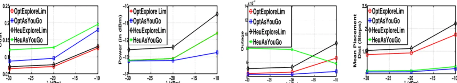
−30 −25 −20 −15 −10 0.05 0.1 0.15 0.2 0.25 ξr(dBm) Cost OptExploreLim OptAsYouGo HeuExploreLim HeuAsYouGo −30 −25 −20 −15 −10 −14 −13 −12 −11 −10 ξr(dBm) Power (in dBm) OptExplore Lim OptAsYouGo HeuExploreLim HeuAsYouGo −304 −25 −20 −15 −10 6 8 10 12 14x 10 −3 ξr(dBm) Outage OptExploreLim OptAsYouGo HeuExploreLim HeuAsYouGo −301 −25 −20 −15 −10 1.5 2 2.5 ξr(dBm) Mean Placement Dist (Steps) OptExploreLim OptAsYouGo HeuExploreLim HeuAsYouGo
Fig. 3. Model-based results for ξo= 10: mean cost per step, mean power per link, mean outage per link and mean placement distance (steps) vs. ξr for
the four algorithms: OptExploreLim, OptAsYouGo, HeuExploreLim, and HeuAsYouGo. The node power in the HeuAsYouGo algorithm was taken to be the
same as the mean node power with the OptExploreLim algorithm. The unit of ξr is actually mW, but here it is shown in dBm.
shadowing variance σ. We keep the HeuAsYouGo transmit power and the per-link target outage equal to the mean power per link and mean outage per link of OptExploreLim. We will only provide results for ξo = 10; with this value
the performance is satisfactory in terms of mean power per node, and the end-to-end outage for a network of length few hundreds of meters. The results are shown in Figure 3. Note that performance of OptExploreLimLearning is not shown in Figure 3, since it has the same asymptotic performance as OptExploreLim (since the policy in OptExploreLimLearning converges to the optimal policy with probability 1).
1) Mean Placement Distance: Pure as-you-go algorithms (OptAsYouGo, HeuAsYouGo of Figure 3) place relays sooner than the algorithms that explore forward before placing a relay (OptExploreLim, HeuExploreLim). This is as expected, since they do not have the advantage of exploring over several locations and then picking the best. A pure as-you-go approach tends to be cautious, and therefore tries to avoid a high outage by placing relays frequently. As ξr(cost of a relay) increases,
relays will be placed less frequently.
2) Mean Power per Link: Increasing ξo(the cost per unit
out-age) will lower outage and hence the transmit power increases. Increasing ξr will place relays less frequently, hence the
transmit power increases. OptAsYouGo has smaller placement distance compared to OptExploreLim and HeuExploreLim and hence it uses less power at each hop; we note, however, that OptAsYouGo places more relays, and, hence, could still end up using more total power.
3) Mean Outage per Link: As ξo, the penalty for outage,
increases, the mean outage per link decreases. As ξrincreases,
the mean outage per link increases because we will place fewer relays with higher inter-relay distances. HeuAsYouGo has outage probability comparable to other algorithms, but it pays in terms of number of relays since it places relays very frequently. We observe that the per-link outage decreases with ξrfor HeuAsYouGo. As ξrincreases, the node power and the
target outage (chosen from OptExploreLim) increases in such a way that the per-link outage decreases.
4) Network Cost Per Step: Cost increases with ξrand ξo.
Op-tAsYouGo has a larger cost than OptExploreLim and HeuEx-ploreLim, owing to shorter links. The cost of HeuAsYouGo in Figure 3 is high due to smaller placement distance. Cost of HeuExploreLim is very close to OptExploreLim.
C. Deployment Experiments By “Virtual” Walking
Now we report our results of carrying out an experimental evaluation of all the algorithms. Based on this evaluation, we select the best algorithm and suitable parameters in order to carry out an actual impromptu deployment, which we report in Section V. Our experimental approach is the following: (i) We deploy 11 TelosB motes, with 9 dBi antennas, equally spaced by 11 meters (δ = 11 m), lashed to trees along one edge of a 110 meter trail, (ii) On command, one by one, each mote broadcasts 2000 packets at each power level from the set S = {−25, −15, −10, −5, 0} dBm, while the rest remain in the receive mode. For each transmit power level of a node, the outage probability at each other receiving node is recorded. Next, we applied the policies to the data. Since we have gathered the outage probabilities of every possible link for all power levels, we have all possible measurements that can be possibly made during an actual deployment. Thus, we can use the measurements to determine the actual network that will be deployed if an agent was to walk along the trail starting from sink at location 1, with the source being at location 11 (the distance between the sensor and the base station is 110 meters). We choose ξo = 10 and ξr = 0.01
for the virtual deployment. For the HeuAsYouGo algorithm, we randomized between two power levels from S so that the mean transmit power per node in the data-based HeuAsYouGo remains equal to that of model-based OptExploreLim. We have also calculated the optimal end-to-end cost of the network graph; we calculated the shortest path from node 11 to node 1 over the weighted network graph where the weight of any potential link consists of the transmit power, outage cost and relay cost, and the weights are available from the field measurements. The cost of the sensor node is not taken into account. Obviously, this approach (OptExploreAll) gives the smallest end-to-end cost (see Table I and the abbreviations in its caption). If we place a relay at location i, (i ≥ 7), the remaining number of steps from there to the sensor location is less than B = 5. In that case, we place one more relay between locations i and 11 such that the cost between 11 and i is minimized. For OptExploreLimLearning, we chose λ0= 0.0321 (optimal cost per step when η = 4, σ = 7 dB).
The OptExploreLim algorithm places relays at locations 5,7,9. It requires B = 5 measurements for placing at each of 5 and 7, see Table I. Then it has to place one more relay, for that it has to measure the cost of the following paths: {(11, 10), (10, 7)},
Algo- Relay No. of mea- Total Po- Sum Total
rithm location surements wer (mW) Outage Cost
OEL 5,7,9 17 0.3542 0.004 0.424 HEL 5,7,9 17 0.3542 0.004 0.424 OELL 4,8,10 15 0.3826 0.006 0.472 OAYG 2,3,4,5,6,8,9 10 0.747 0.018 0.997 HAYG 2,3,5,6,7, 10 0.451 0.586 6.391 8,9,10 OEA 2,6,9 40 0.0704 0.002 0.1204 TABLE I
RESULTS OF VIRTUAL WALKING DEPLOYMENT FOR ONE SIDE OF A TRAIL,
FORξr= 0.01ANDξo= 10. ABBREVIATIONS: OEL-OPTEXPLORELIM,
HEL-HEUEXPLORELIM, OELL-OPTEXPLORELIMLEARNING, OAYG-OPTASYOUGO, HAYG-HEUASYOUGO, OEA-OPTEXPLOREALL.
{(11, 9), (9, 7)}, {(11, 8), (8, 7)} and (7, 7). Hence, OptEx-ploreLim requires 17 measurements to place 3 relays. Similar logic follows for HeuExploreLim and OptExploreLimLearn-ing. The as-you-go algorithms require 10 measurements for 10 steps, and place 7-8 relays. Exploration algorithms place a smaller number of relays and yet produce much better performance compared to pure as-you-go. OptExploreAll (the best algorithm) significantly improves the performance com-pared to exploration algorithms, but makes 40 measurements (between all potential location pairs whose distance is less than or equal to 5 steps). As-you-go algorithms work with measure-ments acquired as the agent walks and, hence, are suboptimal. Hence, the algorithms that employ partial exploration are the ones that require reasonable number of measurements while giving satisfactory performance.
V. PHYSICALDEPLOYMENTEXPERIMENTS
With the experience (on the choice of deployment algorithm) obtained from the virtual deployment experiment discussed in Section IV, we performed some real deployment experiments along a long trail in our campus (not exactly linear in shape, which is the reality in a practical forest environment) with the powerful iWiSe motes (see [8]) equipped with 9 dBi antennas1. We chose ξo = 100, ξr = 1, B = 5 steps, δ = 50 meters,
and S = {−7, −4, 0, 5} dBm. Prcv−min = −97 dBm; the
PER at this RSSI becomes 2% for iWiSe motes (obtained experimentally). In this deployment experiment we used the PER of a link as a substitute for outage probability; this does not violate the basic assumptions of our formulation, and the algorithms remain the same. For η = 4, σ = 7 dB, the optimal average cost per step is 1.0924 (computed numerically using policy iteration). Taking λ0 = 1.0924 (the initial guess), we
performed real deployment experiments with OptExploreLim-Learning. The deployed network is shown in Figure 4. The sink is denoted by the “house” symbol. The two short (50 m long) links account for significant path-loss due to the turn in the trail. After completion of the deployment, we used the last placed node as the source and sent periodic traffic from the source to the sink node at various rates. As the arrival rate increases, the loss probability increases (see Figure 4) due to carrier sense failures and collisions because of simultaneous transmissions from different nodes. For very low arrival rate, the loss probability becomes 0 even though the sum PER under the lone packet model is not 0. This happens because of link level retransmissions and the relatively short outage durations;
1“Actual walking" deployment was done using a deployment tool; see [1].
1500 200 250 300 350 0.01 0.02 0.03 0.04 0.05
Inter−Packet Duration (in ms)
P loss
Fig. 4. Real deployment along a long trail using OptExploreLimLearning
with iWiSe motes, ξo = 100, ξr = 1: five nodes (including the source)
are placed; link lengths, transmit powers, and % outage probabilities are shown; the plot shows variation of end-to-end loss probability with inter-packet duration for periodically generated inter-packets from the source
even if a packet encounters an outage on a link along the path, retransmission attempts succeed with high probability. We see that, even though the design was for the lone packet model, the network can carry 4 packets/second with Ploss≤ 1%.
VI. CONCLUSION ANDONGOINGWORK
In this paper, we have compared the on-field performance of several as-you-go deployment algorithms. Pure as-you-go networks need to be overly cautious, and, hence, deploy far too many relays. Our results suggest that limited exploration based on-line algorithms (such as HeuExploreLim, and Opt-ExploreLimLearning) provide satisfactory performance, at the cost of some additional measurements. In a large forest, we can deploy using OptExploreLimLearning in one trail and use the updated policy in another trail so that the per-step cost of the entire network is optimal. There are several issues left for future study: (i) robust deployment against seasonal variation of propagation, and (ii) deployment in 2D and 3D regions.
REFERENCES
[1] A. Chattopadhyay, A. Ghosh, A.S. Rao, B. Dwivedi, S.V.R. Anand, M. Coupechoux, and Anurag Kumar. Impromptu deployment of
wire-less relay networks: Experiences along a forest trail. available in
www.arxiv.org.
[2] A. Chattopadhyay, M. Coupechoux, and A. Kumar. As-you-go deploy-ment of a wireless network with on-line measuredeploy-ments and backtracking. http://arxiv.org/abs/1308.0686.
[3] A. Chattopadhyay, M. Coupechoux, and A. Kumar. Measurement based impromptu deployment of a multi-hop wireless relay network. In Proc. of the 11th Intl. Symposium on Modeling and Optimization in Mobile, Ad Hoc, and Wireless Networks (WiOpt). IEEE, 2013.
[4] M.R. Souryal, J. Geissbuehler, L.E. Miller, and N. Moayeri. Real-time deployment of multihop relays for range extension. In Proc. of the ACM International Conference on Mobile Systems, Applications and Services (MobiSys), San Juan, Puerto Rico, June 2007, pages 85–98. ACM, 2007. [5] A. Sinha, A. Chattopadhyay, K.P. Naveen, M. Coupechoux, and A. Ku-mar. Optimal sequential wireless relay placement on a random lattice path. Ad Hoc Networks Journal (Elsevier)., 21:1–17, 2014.
[6] A. Bhattacharya, A. Rao, D. G. Rao Sahib, A. Mallya, S.M. Ladwa, R. Srivastava, S.V.R. Anand, and A. Kumar. Smartconnect: A system for the design and deployment of wireless sensor networks. In Proc. of the 5th International Conference on Communication Systems and Networks (COMSNETS). IEEE, 2013.
[7] A. Bhattacharya and A. Kumar. QoS aware and survivable network design for planned wireless sensor networks. http://arxiv.org/abs/1110.4746. [8] http:// www.astec.org.in/ astec/ content/ wireless-sensor-network,.