HAL Id: hal-03016185
https://hal.archives-ouvertes.fr/hal-03016185
Submitted on 20 Nov 2020
HAL is a multi-disciplinary open access archive for the deposit and dissemination of sci-entific research documents, whether they are pub-lished or not. The documents may come from teaching and research institutions in France or abroad, or from public or private research centers.
L’archive ouverte pluridisciplinaire HAL, est destinée au dépôt et à la diffusion de documents scientifiques de niveau recherche, publiés ou non, émanant des établissements d’enseignement et de recherche français ou étrangers, des laboratoires publics ou privés.
Continuous three-dimensional path planning (CTPP) for
complex thin parts with wire arc additive manufacturing
Adama Diourté, Florian Bugarin, Cyril Bordreuil, Stéphane Segonds
To cite this version:
Adama Diourté, Florian Bugarin, Cyril Bordreuil, Stéphane Segonds. Continuous three-dimensional path planning (CTPP) for complex thin parts with wire arc additive manufacturing. Additive Man-ufacturing, Elsevier, 2020, pp.101622. �10.1016/j.addma.2020.101622�. �hal-03016185�
Continuous three-dimensional path planning (CTPP) for complex
thin parts with wire arc additive manufacturing
Adama Diourté
1,a), Florian Bugarin
1,b), Cyril Bordreuil
2,c), Stéphane Segonds
1,d)1Université Fédérale de Toulouse Midi-Pyrénées, Institut Clément Ader – CNRS UMR 5312 – UPS/INSA/Mines Albi/ISAE, 3, rue Caroline Aigle, 31400 Toulouse, France
2Laboratoire de Mécanique et de Génie Civil, Université de Montpellier – CC048, 163 rue Auguste Broussonnet, 34090 Montpellier, France.
a )Corresponding author: [email protected], b)[email protected]
c) [email protected] d) [email protected]
Abstract: Wire arc additive manufacturing (WAAM) is emerging as the main additive manufacturing (AM)
technology used to produce medium-to-large-sized thin-walled parts (order of magnitude: 1 m) at lower cost. To manufacture a part with this technology, the path planning strategy used is the 2.5D. This strategy consists in slicing a 3D model into different planar layers parallel to each other. The use of this strategy limits the complexity of the topologies achievable in WAAM, especially those with large variations in curvature. It also involves several start/stops of the arc as it passes from one layer to another, which induces transient phenomena in which the control of the supply of energy and matter is complex. In this article, a new manufacturing strategy to minimize the start/stop phases of the arc to one unique cycle is presented. The goal of this strategy, called “Continuous Three-dimensional Path Planning” (CTPP) is to generate a continuous trajectory in spiral form for closed-loop thin parts. An adaptive wire speed coupled with a constant travel speed allow a modulation of the deposition geometry that ensures a continuous supply of energy and material throughout the manufacturing process. Using the 5-axis strategy coupled with CTPP allows the manufacture of closed parts with a procedure to determine the optimum closing area and parts on non-planar substrates useful for adding functionalities to an existing structure. Two geometries based on continuous manufacturing with WAAM technology are presented to validate this approach. The manufacturing of these parts with CTPP and several numerical evaluations have shown the reliability of this strategy and its capacity to produce complex new shapes with a good geometrical restitution, difficult or impossible to reach today using 2.5D with WAAM technology.
Keyword: Wire arc additive manufacturing (WAAM), Toolpath generation, 5-axis strategy, Geodesic distance, Closed parts
1. Introduction
Wire arc additive manufacturing (WAAM), is nowadays established among the other additive manufacturing (AM) technologies as the technological solution allowing to manufacture at a lower cost, thin-walled structures of large dimensions with a medium geometric complexity [1]. An excellent buy-to-fly ratio makes WAAM a very attractive technology for the aeronautic industry [2] . However, WAAM is not yet widely deployed in the industrial field due to certain technology-related issues such as distortion, residual stresses related to contraction during molten pool cooling and manufacturing strategy. Indeed, it has been shown by Ding et al. [3] that the manufacturing strategy is closely linked to the deposit and therefore automatically linked to the quality of the final part. Hence there is a need to implement a path planning strategy, applicable to a large number of geometric shapes while guaranteeing good quality of the manufactured part. Since arc start and stop phases generate important defects in the final part, the optimization criteria for tool path planning is the minimization of arc start/stop phases.
technologies, is the 2.5D. This strategy consists of dividing any 3D model, into several layers parallel to each other in a construction direction perpendicular to them. The distance between layers can be constant, called uniform slicing, or variable, called adaptive slicing. The adaptive slicing set up by Ma et al. [4] allows an automatic adjustment of the distance between the layers and so improves the geometric approximation (Figure 1).
(a) (b)
Figure 1 : 2.5D strategy for additive manufacturing. (a) Uniform slicing. (b) Adaptive slicing
Then the 2D layers resulting from this slicing are filled with different patterns [5–7] such as raster, zigzag or contour. This 2.5D strategy works perfectly for powder or polymer-based AM but must be adapted to the needs of WAAM due to the higher deposition rate (the amount of material deposited during a given time: several kg/h). Moreover, this strategy requires a good control of the deposit height on each layer, however because of the arc start/stop phases, this requirement is not respected. For example, for the deposition of a layer, during the priming phase the deposition height is higher than in the central zone of the weld bead and lower during the de-priming phase. This leads to issues with the variability of the deposit. According to Zhang et al. [8] this is due to heat dissipation in the substrate during priming, penetration during welding is lower which explains a higher height; and the drop-in height at the end of the weld bead is due to the flow of molten metal. This variation in height influences the following layers, and after a few layers, the difference increases [9] and ends up giving a structure that does not conform to the original geometry (Figure 2).
Figure 2 : Arc start/stop phases in closed circuit parts leads to geometry defects [9].
In addition to the arc start/stop phases, tool paths with discontinuities, sharp corners and overlaps, influence the quality of the deposit, and therefore of the part. To solve these problems, several path planning studies for massive structures have been carried out by Ding et al [3,5], and more recently Michel et al [10], to increase the quality of parts manufactured with WAAM from the 2.5D strategy. There are also less versatile strategies, developed mainly for certain structures that are generally thin-walled. Among these strategies, we can mention the enclosed structures of Kazanas et al [11] whose surface is described by a mathematical equation (Figure 3) and the cross structure with straight walls of Mehnen et al [12]. These solutions require the implementation of a specific strategy for each of the structures to be manufactured, which takes a long time and does not meet the requirements of AM [10].
Figure 3 : Closed part manufactured with mathematical equations [11][13].
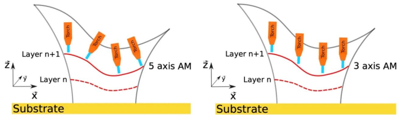
In view of the work carried out in recent years in the field of path planning in WAAM, the focus has been on developing methods to best adapt the 2.5D strategy to the technical constraint associated with the process. However, this strategy involves a 3-axis path planning strategy, which means limiting the complexity of the structures that can be made. Indeed, this strategy leads to a poor surface finish and poor geometry accuracy due to the staircase effect inescapable for curved structures and non-planar boundary surfaces (Figure 1). In powder-based AM technologies, in order to reduce the staircase effect, the layer height is reduced. In polymer-based AM, in addition to the possibility of reducing the layer height, there are other methods of reducing the staircase effect, such as CurviSlicer [14] , which makes it possible to curve conventional layers from 2.5D in such a way that it can follow the natural slope of the input surface. These solutions are not suitable for WAAM because of its higher deposition rate. In general, the motion system used is a 6-axis robot, which means that 2.5D strategy does not use all the degrees of freedom offered by the system. Hascoët et al [15] have demonstrated that 5-axis manufacturing is a sustainable solution for inclined or varying curvatures structures. The advantage of the 5-axis comes from the orientation of the nozzle, in fact with 3 axis paths the nozzle always remains perpendicular to the layer to be deposited, while for 5 axis paths the nozzle always remains tangent to the surface of the part (Figure 4). Being tangent to the surface of the part makes it possible to improve the accuracy of parts with a variation in curvature therefore avoiding the staircase effect [15] . So, to increase the complexity of the structures that can be manufactured by WAAM while avoiding staircase effects and thus maintaining a good geometry accuracy, it is necessary to implement a new path planning strategy different from the 2.5D one and that fully uses 5-axis.
Figure 4 :Differences between 5-axis and 3-axis strategies
1.2. Contributions
deposition height constant, in CTPP the deposition is locally modulated to best represent the geometric shape to be manufactured and limit the number of arc start/stop phases. Indeed, one of the advantages of WAAM over other AM technologies is to be able to modulate the deposition height at any time, and not at each layer as with the powder-based technologies. The deposition modulation is set in the interval [hmin, hmax] where hmin is the minimum deposition
height and hmax the maximum deposition height (Figure 5).
Figure 5 : Modulation of the deposition height on a weld bead in a fixed interval
This deposition modulation interval depends on the control of the different WAAM parameters. By integrating deposition modulation and a 5-axis approach, this strategy allows access to the manufacture of new complex shapes with WAAM, such as shapes with a non-planar boundary, thanks to curved path, or enclosed shapes with minimum arc start/stops (Figure 6).
(a) (b)
Figure 6 : (a) Open part with a non-planar boundary surface. (b) Closed part
The benefit of structures with non-planar boundary surfaces, such as the one shown in Figure 6.a, is to allow the fabrication of parts on curved surfaces, such as pipes. Thus extending the surfaces on which it is possible to build and make the process more versatile for adding functionality to existing structures [16].
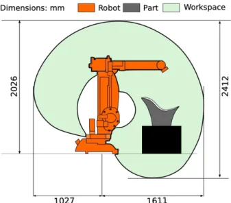
In this work, a six-axis robotic arm holds the welding torch. The robot is controlled with six degrees of freedom (X, Y, Z, RX, RY, RZ) which are the three translations and the three rotations linked to the Cartesian frame [17]. Figure 7 shows a diagram of the six-axis robot with a vertical cross-section of the workspace, the dimensions of this workspace allow the manufacture of workpieces of the size of a meter. The wires feed speed WFS and the robot travel speed TS are adapted in order to locally achieve an appropriate deposit height. This makes it possible to produce complex open/closed parts without interrupting the weld bead, which will allow the manufacture of new shapes and reduction of the manufacture time due to the single arc start/stop. In this work two geometrical concepts will be used:
• Open Parts: defined as geometric shapes with at least one free edge in addition to the one in contact with the substrate.
• Closed Parts: defined as geometric shapes with a single free edge, the one in contact with the substrate.
maximum deposit hmax minimum deposit hmin
Subst rat e x z y z x y
Figure 7 : Six-axis robot with the vertical cross-section of the workspace and the print scale of the part
The goal of this paper is to establish a continuous path in spiral form for closed-loop thin parts. These parts can be closed or open with non-planar boundaries as described above. The continuous path is step up with a constrained deposition height modulation in an interval [hmin, hmax]. To achieve this goal, the article will be as follows:
• Section 2: First the conditions necessary for a part to be manufactured using the CTPP strategy are defined. Then the CTPP strategy is presented;
• Section 3: Two application examples of CTPP are presented, firstly an open part and then a closed part.
• Section 4: The ability to build complex parts with WAAM technology using the CTPP strategy is exposed
• Conclusion and perspectives are presented in the final section.
2. Continuous Three-dimensional Path Planning
In CTPP, as in all AM strategies, the part is first modelled using CAD software. Once the structure is modeled, it is converted to STL format. The STL format represents the geometry by a triangular mesh, each triangle is described by the coordinates of the three vertices that compose them and a unit vector to indicate the external normal to the facet. The representation of geometry in this format allows us to use the different algorithms necessary for the realization of the strategy. In the following section 2.1, the type of geometries that can be manufactured using CTPP will be described. Then CTPP will be detailed in the following sections 2.2-2.5.
2.1. Parts with single branch skeletons
The first condition to be respected by a part, for the use of the continuous tool path, is that the skeleton resulting from its skeletonization must have a single branch. An example of a single branch part, for which a spiral path is feasible and a multi-branch part, for which two spiral paths are necessary on the upper half, is shown on Figure 8.
(a) (b)
Figure 8 : Skeletonization. (a) Single branch skeleton. (b) Multi branches skeleton.
To ensure a continuous path, i.e a single arc start/stop of the electrical arc, the skeleton of the part must contain a single branch. However, with the possibility of manufacturing on non-planar surfaces offered by the CTPP, our method can be applied to each of the branches independently (using a decomposition method) for the manufacture of multi-branch structures with several arc start/stops.
Skeletons are tools to extract topological information from a given shape. The skeleton can be imagined by placing a sphere inside the part, this sphere must remain tangent to at least two points of the contours inner surface at all times. The trajectory of the sphere’s center, as it is displaced through the part, determines the skeleton, an example of this is given Figure 8.a. This method allows a one-dimensional representation of the shape while retaining its topological information.
There are four major skeletonization methodologies in the literature: distance transform field-based methods [18–20], Voronoi diagram-based methods [21–23], thinning-based methods [24,25] and mesh-based methods [26,27]. As the parts used in this study are modelled in STL format, mesh-based methods are more appropriate and will be used. For more precision on these algorithms you can refer to [26]. The algorithms are implemented in the libraries presented in section 3.
Parts with a single branch skeleton can be open or closed, as illustrated in Figure 6. That is why the CTPP is composed of two modules, a first module dedicated to the manufacture of open parts and a second one for closed parts. This separation is carried out because the two types of geometry don’t have the same needs. Indeed, for closed parts, in addition to generating a manufacturing trajectory, it is also necessary to determine the optimal zone for closing the part. The determination of this zone will allow a continuous path planning for closed parts.
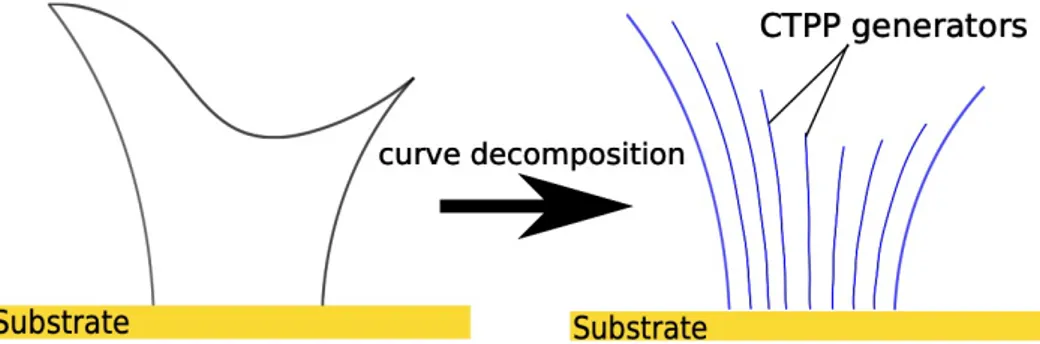
2.2. Decomposition by curved generators
The fundamental idea of the CTPP is the decomposition of the part by a set of curves. In the case of an open part these curves connect the sections limiting the upper and lower surfaces. In the case of closed structures, the curves connect the lower section to the closing zone. The set of curves is called “generators’ in the CTPP strategy, by analogy to the generators of a ruled surface. Therefore, in the CTPP strategy, a generator is defined as a succession of points connecting two limiting zones of a part (Figure 9) according to a criterion defined in section 2.2.1. Subst rat e x z y Substrate CAO enveloping path Substrate CAO enveloping path Substrate CAO enveloping path Substrate CAO Skeleton points on enveloppe points on surface points on skel eton
Substrate CAO points on enveloppe points on surface Pi Pi+1 P'i P'i+1 Substrate Pi Pi+1 P'i P'i+1 CAO Skeleton points on enveloppe points on surface points on skel eton
Substrate CAO Skeleton Sphere Sphere center Substrate Substrate
Figure 9 : CTPP generators: decomposition of an open part by curved generators
In the following paragraph, the decomposition of parts into generators is presented. First the decomposition of open parts will be discussed; followed the decomposition of closed parts. As previously mentioned, these parts require different strategies leading to two separate modules within the CTPP strategy.
2.2.1. Open Parts
Let us consider Ω the surface representation by the triangular mesh, of the structure to be manufactured and ¶Wupper and ¶Wlower the upper and lower sections of the structure. The first step consists in discretizing the lower section into npts points with a constant angular distribution
around the vertical axis z (Figure 10.a).
(a) (b)
Figure 10 : Discretization of the boundary sections of the structure. (a) Discretization of the lower section by constant angular distribution. (b) Discretization of the upper section by minimizing the geodesic distance between 𝑃!!"#$%and the
upper section
The points resulting from this discretization are noted 𝑃!!"#$% with 𝑖 ∈ [1, 𝑛"#$]. Then the upper section is discretized using the notion of geodesic distance. The geodesic distance between two points s and t noted 𝜑(s, t), is the shortest path on the surface Ω that connects these two points [28–30]. For discretization of the upper section, also in npts points, at each point 𝑃!!"#$%, the
𝑃!&''$% point associated with it is the one that minimizes the geodesic distance between 𝑃!!"#$%
and the upper section ¶Wupper (Eq.1) (Figure 10.b). The geodesic distances connecting the pairs of points [𝑃!!"#$%, 𝑃!&''$%] are the generators G= {𝒈𝟏, . . . , 𝒈𝒏𝒑𝒕𝒔} of the structure in the CTPP.
𝑃+!""#$=, ∈ /0min
!""#$𝜑(𝑃+%&'#$, 𝑃) Eq.1
The determination of generators by calculating geodesic distance can lead to uncovered areas for certain geometric shapes. Indeed, geodesics always passing through the shortest path, some areas may not be covered (Figure 11).
Substrate x z y ) Ωlower ϭ Ωupper ϭ Substrate x z y Generator Piupper Pilower
Figure 11 : Illustration of several areas not covered by the generators on an open part.
These areas are detected and filled to achieve a complete decomposition of the model into generators. To detect uncovered areas, two adjacent generators are taken. A triangular mesh 𝜓 is generated from these two generators, then an error 𝜀 calculation is made. The error 𝜀 represents the difference between the generated surface 𝜓 and the surface portion of Ω delimited by the two generators called S’ (Figure 12.a).
(a) (b)
Figure 12 : (a) Detection of uncovered areas after calculation of curved generators. (b) Filling of uncovered area by projection of median curve.
The calculation of 𝜀 is done as follows:
For each vertex v of the mesh 𝜓 the minimum distance from the vertices of S’ is calculated as shown in Eq.2.
𝑑(𝑣, 𝑆1) = min
2(3 4(‖𝑣 − 𝑣′‖ Eq.2
Where ‖. ‖ is the Euclidean norm. From this definition, the error 𝜀 is defined as shown in Eq.3. 𝜀 = max
2 3 5𝑑(𝑣, 𝑆
1) Eq.3
The error 𝜀 is therefore the maximum gap between the two surfaces. If this gap is greater than a user-defined threshold value 𝜀', a new generator is inserted between the first two generators. The new generator is determined by projecting on S’ the median curve C between the first two generators according to the vector formed by the vertex pair (v,v') which allows the calculation of 𝜀 (Figure 12.b). The new generator is added to the list G, and detection and filling is repeated on the next two generators and so on until an error 𝜀 ≤ 𝜀' is obtained over the entire surface. After filling the list of generators is G= {𝒈𝟏, . . . , 𝒈𝒏𝒑𝒕𝒔(𝒏𝒇𝒊𝒍𝒍𝒊𝒏𝒈}, and therefore the open part is
decomposed by generators (Figure 9). 2.2.2. Closed Parts
In the case of closed parts, there is no section to define an upper limit, it is therefore necessary to determine the optimal closing zone, such that the part can be manufactured with a single
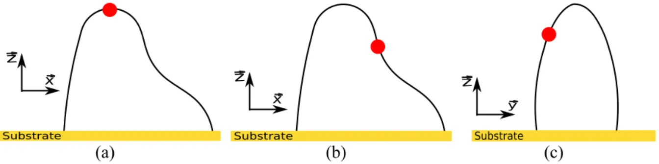
weld bead, whose deposit height varies between [hmin, hmax]. For example, in the case of a half sphere, the optimal closing zone is at its apex as the geometry is axisymmetric. On the other hand, for the structure illustrated in Figure 13, a criterion must be set up to determine whether one closure area is better than another among a set of possibilities.
(a) (b) (c)
Figure 13 : Illustration of different possible closing zones for a closed part.
In order to find this optimal closing zone, the lower limit surface ¶Wlower is discretized into npts points with a constant angular distribution around the z axis as in the case of open parts (Figure 14).
Figure 14 : Search for the optimal closing zone of a closed part. For each vertex of the mesh, the minimum geodesic distance is calculated with respect to the base of the structure. The optimal end point is the point that maximizes these minimum
geodesic distances.
For each of the nvertex points of the Ω mesh of the closed geometry, the minimum of the geodesic distances with respect to the npts points of the ¶Wlower section is calculated. The optimal point (Eq.4), chosen for the closure, corresponds to the point on Ω that maximizes the smallest geodesic distance from all npts points of the lower section ¶Wlower.
𝑃;<=+>?@ = max( min, ∈ 0(𝜑4P , 𝑝+%&'#$7)) Eq.4
It is necessary to minimize the difference between generator lengths to ensure that the deposition height remains in the range [hmin, hmax]. This search criterion to determine the optimal point is a consequence of the feasibility criterion, which will be detailed in section 2.5. Once the optimal point has been found, the generators of the structure are defined using the same method as for open parts, considering the closing point as the upper limit section ¶Wupper.
2.3. Discretization of generators
Once the generators are obtained, the objective is to generate a continuous spiral trajectory whose thickness varies in an interval compatible with the characteristics of the bead deposition process (deposition modulation interval). The generators are therefore discretized to achieve this goal. The procedures explained in this section are set up in such a way that the points belong
Substrate x z Substrate x z Substrate z y Geodesic distance
Potential end point : Pj
2.3.1. Height discontinuity
Firstly, the continuous path must be initiated. On the first revolution, the deposition height is linearly modified between hmin and hmax . A discontinuity occurs at the beginning of the second pass (Figure 15.a). This height discontinuity is due to the fact that bead deposition cannot start at zero height due to the limited modulation range of the deposit. This discontinuity in height must be eliminated to avoid its propagation and accentuation over the layers.
(a) (b)
Figure 15 : Discontinuity of deposition height when setting up the continuous path. (a) Appearance of a discontinuity at the beginning of the second layer. (b) Increase in the difference between the minimum and maximum overall height achieved
over a given number of revolutions.
To eliminate this height discontinuity during the first turns of manufacture, deposition modulation is used. Considering h as the average deposition height over a revolution and Δhj
the difference between the minimum and maximum overall height reached over j revolutions (Figure 15.b).Through the different revolutions, ∆𝒉𝒋 = 𝒋 ∗ ( 𝒉𝒎𝒂𝒙− 𝒉𝒎𝒊𝒏) increases, which leads to two cases:
• ∆𝒉𝒋< 𝒉
For the layers in this case, the points are displaced along the generators according to a linear distribution between hmin and hmax.
• ∆𝒉𝒋≥ 𝒉.
As soon as this condition is reached, the point distribution range is changed. The first layer satisfying this condition are distributed linearly between hmin and hmin+h, this creates a difference of h between the first point of this layer and the last one. Then for the next layer, the average deposition height h is added to the points in the previous layer. This results in a layer with a regular deposit on which the discontinuity has been eliminated (Figure 16).
(a) (b) (c)
Figure 16 : Generation of a continuous path on an open part. (a) Elimination of height discontinuity and calculation of remaining length on generators. (b) Discretization of generators. (c) Setting up the continuous path.
For example, using the following modulation range [hmin = 0.9h, hmax = 1.1h] the number of layers required to eliminate the discontinuity is 6 layers (Table 1).
Table 1 : Search for the number of layers necessary to eliminate the setup discontinuity
Layer j Maximum height
reached Minimum height reached ∆𝒉𝒋 1 hmax hmin 0.2*h 2 2*hmax 2 *hmin 0.4*h 3 3*hmax 3*hmin 0.6*h 4 4*hmax 4*hmin 0.8*h 5 5*hmax 5*hmin h 6 6*hmax 6*hmin 1.2*h
The number of nstepLayers layers required to eliminate the discontinuity depends on the
modulation range. The larger the modulation range achievable with the process, the less layers are needed to eliminate the discontinuity. A modulation of ±10% around an average value h is ensured with good precision within our research structure, i.e. hmin = 0.9h, hmax = 1.1h.
2.3.2. Calculation of the number of remaining layers
Once the height discontinuity is eliminated, the number of revolutions required to manufacture the remainder of the part is calculated. The remaining length L= {𝒍𝟏, . . . , 𝒍𝒏𝒑𝒕𝒔(𝒏𝒇𝒊𝒍𝒍𝒊𝒏𝒈 } of each
generator after elimination of discontinuity is first determined (Figure 16.a). The number of layers remaining to finish the part is determined by dividing the minimum length of L by the minimum deposit hmin (Eq.5). If the quotient of this ratio is not an integer, it is rounded down to the lower integer value.
𝑛B?CDEF= 𝑓𝑙𝑜𝑜𝑟(GHI (B)L
)*+ ) Eq.5
The number of nLayers layers thus known, all the lengths calculated previously are divided by
this number in order to obtain a discretization of each generator with a step between the points of D= {𝑑/ = 𝒍𝟏
1NOP$%Q, . . . , 𝑑2=
𝒍𝒏𝒑𝒕𝒔R𝒏𝒇𝒊𝒍𝒍𝒊𝒏𝒈
1NOP$%Q } (Figure 16.b). Finally, the points are connected to
each other to form the continuous manufacturing path (Figure 16.c). 2.4. Orientation of robot during manufacturing
In the previous sections, a continuous three-dimensional path planning strategy was implemented for both open and closed type structures. To complete this strategy the orientation of the nozzle along the continuous weld bead deposit must be determined.
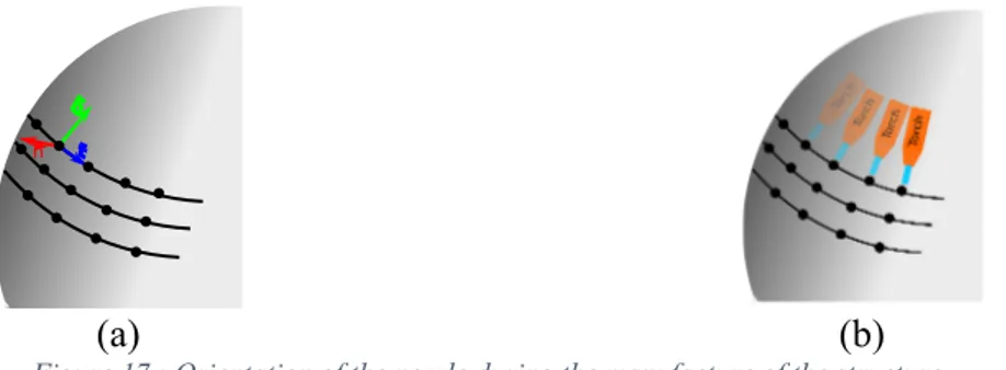
As we have a 6-axis robot arm to move and orient the nozzle, 5-axis manufacturing is used. The structures resulting from the CTPP can have a high variation in curvature, so the choice of the 5 axis is necessary to ensure a good quality of the parts. In order to determine the orientation of the nozzle during manufacturing, a direction of construction is associated with each point of the continuous path. This direction is obtained by calculating at each point, the cross product between the surface normal 𝒏XX⃗ and the vector 𝒕⃗ pointing to the next point (Figure 17.a).
(a) (b)
Figure 17 : Orientation of the nozzle during the manufacture of the structure.
This allow us to obtain the different orientations of the nozzle during the manufacture of structure (Figure 17.b). The orientation of the nozzle is not necessarily along the calculated generators. So, to find the real deposit during the fabrication of the structure, for each point the deposit di from D is projected on his direction of construction (Figure 18). The deposit is
therefore 𝐻 = \ℎ/,/ = 𝑑/∗ cos 𝜃/,/, … … , 𝑑𝒏𝒑𝒕𝒔(𝒏𝒇𝒊𝒍𝒍𝒊𝒏𝒈∗ cos 𝜃𝒏𝒑𝒕𝒔(𝒏𝒇𝒊𝒍𝒍𝒊𝒏𝒈 ,1!OP$%Q`.
Figure 18 : Calculation of the true deposition height during manufacture.
After the orientation of the nozzle has been determined, there is a risk of collision between the workpiece being manufactured and the nozzle, especially for closed structures. In this case a reorientation of the nozzle is made by rotating around the vector 𝒕⃗ at the points where the collision occurs. Collision detection is done by calculating, at a given time, the intersection between the part being manufactured, modelled by a tube of radius RTube centered on the
trajectory, and the robot arm carrying the nozzle, modelled by a cylinder centered on its axis and of radius RArm equal to the maximum radius between the outer surface and its axis [31].
2.5. Feasibility criterion
Due to a limitation of the modulation range imposed by the process, not all structures are achievable with a continuous path. The part to be manufactured must satisfy the criteria given by Eq.6 .
max(𝐻) ≤ ℎ>?S 𝑎𝑛𝑑 min(𝐻) ≥ ℎ>+T Eq.6
This ensures that the deposition during fabrication is always within the modulation range imposed by the manufacturing process. One consequence of this criterion is that the complexity of the structures that can be fabricated by the CTPP depends on the modulation range and therefore on the control of the parameters of the manufacturing process. The larger the modulation range, the more complex the parts that can be produced. The feasibility criterion is a tool, to assess upstream, whether the structure is manufacturable with a continuous path from a given modulation range.
t n b t n b
b
ϴi,j generator build direction di hi,j Layer j-1 Layer j3. Application of CTPP
The proposed solution CTPP has been implemented using PYTHON and C++. Two open source libraries were used, the first one “The Computational Geometry Algorithms Library” (CGAL) [32] is a software project that provides easy access to efficient and reliable geometric algorithms. It is used in various fields requiring geometric computation, such as geographic information systems, computer aided design and robotics. In this work it is used to calculate the geodesic distance and to carry out the skeletonization. The second library “The Visualization Toolkit ” (VTK) [33] is software for manipulating and displaying scientific data. It is used for visualizing the continuous path and nozzle orientation along this path.
To validate the CTPP strategy, two structures are modelled, an open part and a closed part (Figure 19). The open part chosen here, in addition to having a non-planar boundary, also has several curvature variations and better represents the benefits of CTPP than the part used to illustrate the methodology (Figure 6.a).
(a) (b)
Figure 19 : Illustration of two complex structures. (a) Open part 1. (b) Closed part.
3.1. Open part
The open part has several variations of curvature, a non-axisymmetric shape and a variable section (Figure 20). The base of the structure is not perpendicular to the substrate. Therefore, the use of the 5-axis strategy imposes a starting angle non-perpendicular to the substrate. As the nozzle must remain tangent to the surface of the structure.
Figure 20 : Different points of view of the CAD of the open part 1 to be manufactured.
The strategy described in section 2 is applied to this structure with the parameters indicated in Table 2.
Table 2 : The different parameters provided and calculated during the application of the CTPP on the open part.
Minimum deposit 1.8 mm
Maximum deposit 2.2 mm
Average deposit 2 mm
Generator of maximum length 178 mm
Generator of minimun length 152 mm
Number of layer 84
Feasibility criterion Valid
After application of the CTPP strategy, the continuous path obtained is illustrated in Figure 21. This manufacturing path consist of 84 layers with an average deposition of 2 mm and a modulation of ±10% around this value.
Figure 21 : Continuous three-dimensional path obtained after application of the CTPP on the open part 1.
Once this trajectory has been obtained, before proceeding to manufacture the part, a check of the nozzle orientation is carried out. For this purpose, a cylinder with a radius R is modeled to represent the nozzle during manufacture. The axis of the cylinder is taken in such a way that it coincides with the direction of construction calculated at each point of the continuous path. Figure 22.a shows the Frenet-Serret frame associated with each point, used to determine nozzle orientation. Figure 22.b and Figure 22.c show two examples of nozzle orientation at different times during manufacture.
(a) (b) (c)
Figure 22 : Illustration of different nozzle orientations during the manufacture of the open part 1. (a) Frenet-Serret frame associated with each point allowing to orientate the nozzle. (b)-(c) Orientation of the nozzle at different time during the
manufacture.
Once the manufacturing trajectory has been obtained and the nozzle orientation approved, the next step is to manufacture the part.
3.2. Closed parts
For the closed structure, before generating the manufacturing path, the optimal closing point must first be determined. The structure illustrated in Figure 23 is symmetrical with respect to the (Oxz) plane, but not with respect to the (Oyz) plane. It has a variable section and a variation in curvature. The CTPP is applied with the same deposition parameters as those indicated in Table 2.
Figure 23 : Different points of view of the CAD of the closed part.
The search for the closing point is carried out following the procedure described in section 2.2.2. In our case, the closing point’s coordinates, calculated according to our criterion, are (-40.47, -1.05, 258.64), this point is shown in Figure 24.a. As the structure is symmetrical with respect to the (Oxz) plane it is consistent that the optimal point is also in this plane. A slight deviation from this plane can be observed because the optimal point search solution is calculated on the existing mesh. The optimal closing point is not at the top of the structure as one might intuitively think, but leans towards the side of the structure with the variation in curvature. This is a consequence of minimizing the gap between the different generators.
(a) (b) (c)
Figure 24 : Generation of a continuous path on the closed part. (a) Optimal closing point of the part according to the developed criterion. (b)-(c) Continuous manufacturing path on the closed after application of CTPP from different angles.
Once the optimal closing point has been obtained, the continuous manufacturing path is generated on the surface (Figure 24.a and Figure 24.b). The parameters calculated during the application of the CTPP are shown in Table 3.
Table 3 : The different parameters calculated during the application of the CTPP on the closed part.
Generator of maximum length 303 mm
Generator of minimun length 323 mm
Number of layer 168
3.3. Deposition height comparison between CTPP and 2.5D strategies
To see the advantage of manufacturing a part with CTPP over the 2.5D strategy, both strategies are applied to the open part. Figure 25 shows a deposition height map for the two manufacturing methodologies. For the 2.5D strategy, the workpiece is sliced by multiple planes parallel to each other, with their normal directed along the z-axis and separated from each other by 2 mm. Figure 25.a represents a mapping of the minimum distance between two successive layers. The first thing to be noted on this figure is the fact that the deposition height is mostly around 2 mm except in areas with strong variations in curvature. Based on these results the constraint of the modulation range [2 mm±0.2 mm], is not respected. The second thing to be noted is that the 2.5D strategy does not make it possible to accurately reproduce the non-planar shape of the upper boundary (black area in Figure 25.a). This and the start/stop phases of the arc both affect the accuracy of the part to be manufactured.
(a)
(b)
Figure 25 : Deposition comparison between CTPP and 2.5D strategies. (a) Deposition height with 2.5D strategy. (b) Deposition height with CTPP strategy.
Figure 25.b represents a mapping of deposition height using the CTPP strategy with the parameters indicated in Table 2. The deposition height constraint is respected over the entire part with a minimum deposit of 1.8 mm and maximum of 2.1 mm. Small deposits are concentrated in areas where the upper boundary is low and large deposits concentrated in areas
where the upper boundary is high. This makes it possible to anticipate the non-planar shape of the upper boundary right from the start of the manufacture of the part, thanks to curved path. In addition to this, a continuous manufacturing process allows the reduction of start/stop phases and therefore reduces the defects linked to these phenomena.
Consequently, a more accurate manufacturing of parts with curvature variations and non-planar boundaries can be obtained with the CTPP method compared to the classical 2.5D strategy. Moreover, today it is experimentally impossible to achieve this structure using the 2.D strategy with the deposition parameters indicated in Table 2.
4. Experimental validation
In this section the experimental validation using two open parts is presented, the first is the part used to illustrate the CTPP strategy (Figure 19.a) and the second is a modified version of the closed part (Figure 26.). The Closed part was not selected because of the risk of collapse when converging to the closed area. Indeed, as the part approaches this closing zone, the manufacturing being continuous and therefore without cooling periods, the part overheats and collapses. A thermal study must first be conducted to evaluate the impact of the CTPP on the part to be manufactured, to identify the areas of overheating and implement strategies to prevent collapse. One approach would be to pause in the overheated areas to cool down the part.
(a) (b) (c)
Figure 26 : Open part 2. (a)-(b) Different points of view of the CAD. (c) Continuous three-dimensional path on the part..
As a movement system, we have a 6-axis robot arm offering great flexibility of orientation and a large working space. A welding system based on the cold metal transfer technology (CMT) developed by Fronius [34] is attached to the robot arm. To modulate the deposition height within a fixed interval, the wires feed speed and the robot travel speed will be modified. WAAM parameters can be divided into three categories: the wire feed speed (WFS), heat source power (voltage U and current I) and path parameters (travel speed (TS), layer height (LH), layer width (W)). A relationship exists between these parameters and the diameter of the wire (Eq.7) [15]:
𝐿𝐻 = ../"#$%& .012
3.0.42 Eq.7
Figure 27 and Figure 28 show the two open parts made using WAAM technology in steel. These structures are made with a single weld bead from beginning to end using a single initiation/extinction of the arc. This allows the idle times inherent to the 2.5D strategy to be
Figure 27 : Different points of view of the open part 1 manufactured with WAAM technology using the continuous path resulting from the CTPP strategy.
Figure 28 : : Different points of view of the open part 2 during the manufacturing process and after, with WAAM technology using CTPP strategy.
Indeed, with the 2.5D strategy, in practice, a waiting time is applied between different layers to avoid overheating the previous layer thus reducing distortion of the final part. By eliminating these waiting times, the CTPP makes it possible to shorten the manufacturing time of structures and the use of the 5-axis strategy ensures good part quality without the use of supports. The manufacture of the part shown in Figure 27 took 1 hour, with a continuous deposition over 84 revolutions for a structure height of 160 mm and an average deposition height of 2mm. For the second part (Figure 28), the manufacture took 8 hours over 74 revolutions for a structure height of 225 mm with an average deposit of 3.1 mm.
The variations in curvature on both structures are well transcribed and do not have a staircase effect (Figure 1). On the surface of the structure in Figure 29, it can be seen that some areas have a smooth surface and others a rough surface. These rough areas are due to the stick-out distance, which is the length of the wire from the nozzle outlet to the workpiece. Indeed, during the deposition of a layer in the 2.5D strategy, the stick-out distance remains constant whereas in CTPP, the modulation of the deposition height implies a local variation of this stick-out distance. This is why artifacts appear on some areas of the surface. However, better control of wire feed speed, travel speed and the stick out distance would limit their occurrence.
Figure 29: Illustration of areas with different surface conditions on the open part 1. (red) rough surface. (green) smooth surface.
In order to evaluate the reliability of the trajectory generated with the CTPP strategy, a comparison between the surface from the trajectory and the CAD part is made. Figure 30 represents the surface generated from the established manufacturing path and its deviation from the open part shown in Figure 20. The gap between the two surfaces is within a range of [-0.2;0.2]mm which is an acceptable error compared to the dimensions of the part. These differences in deviations are concentrated in the areas where the curvature variations are found, but on the majority of the surface the deviations are close to zero as shown in the histogram provided in Figure 30. Finally, the manufacturing trajectory developed using the CTPP strategy reproduces with good fidelity the structure to be manufactured.
(a) (b)
(c) (d)
Figure 30 : Comparison between the surface from the CTPP and the CAD part of the open part 1.
Uneven surface
5. Conclusion
The complexity of the structures achievable with WAAM is limited in the 2.5D trajectory planning strategy. To manufacture structures with varying curvatures, non-planar upper boundaries or closed parts, with good quality, it was necessary to implement a 3D path planning strategy. In this article a new parts manufacturing strategy for WAAM was presented. This method takes advantage of certain technological aspects of WAAM technology so far unexploited in path planning: modulation of the weld bead height and use of the multi-axis printing configuration (5 axis).
This strategy, called Continuous Three-dimensional Path Planning (CTPP), is a 3D trajectory generation strategy for complex structures with thin walls and closed-circuits. CTPP is based on modelling the surface of the part using different generators. These generators are then discretized so that they can satisfy the deposit height modulation imposed by the manufacturing process while eliminating the height discontinuity induced at the start of manufacturing. The points resulting from this discretization are then linked together to form a continuous manufacturing path for the part. A part feasibility criterion and an optimal closing zone criterion for closed parts are implemented for the use of this strategy. Finally, the orientation of the nozzle to use multi-axis printing throughout the manufacturing process is determined.
This strategy is validated thanks to the production of parts (Figure 31) with a single start/stop of the electric arc as a result of a single continuous manufacturing path. By eliminating the start/stop cycles present in the 2.5D strategy, the manufacturing time of the parts is reduced as well as the heat input related to these cycles.
Figure 31 :Parts manufactured with WAAM technology using the continuous path resulting from the CTPP strategy. (Left) Part 2, (Center) Part 1: Height= 16cm, (Right) Part 1 with a scale factor of 2.5.
Several numerical evaluations have been carried out to justify the reliability of this strategy, first a comparison between the deposition using the developed strategy and the classical 2.5D has been carried out. Then the good restitution of the part to be manufactured was evaluated by comparing the differences between the surface resulting from the manufacturing trajectory and the original CAD part.
For the experimental production of closed parts, the collapse of the structure during closure must still be managed. A thermal modelling of these areas would provide additional information for waiting times for cooling purposes to prevent collapse.
6. References
[1] S.W. Williams, A.C. Addison, F. Martina, G. Pardal, J. Ding, P. Colegrove, Wire + Arc Additive Manufacturing, Mater. Sci. Technol. 32 (2015) 641–647.
https://doi.org/10.1179/1743284715y.0000000073.
[2] J. Ding, P. Colegrove, J. Mehnen, S. Ganguly, P.M.S. Almeida, F. Wang, S. Williams, Thermo-mechanical analysis of Wire and Arc Additive Layer Manufacturing process on large multi-layer parts, Comput. Mater. Sci. 50 (2011) 3315–3322.
https://doi.org/10.1016/j.commatsci.2011.06.023.
[3] D. Ding, Z. Pan, D. Cuiuri, H. Li, A tool-path generation strategy for wire and arc additive manufacturing, Int. J. Adv. Manuf. Technol. 73 (2014) 173–183.
https://doi.org/10.1007/s00170-014-5808-5.
[4] W. Ma, W.-C. But, P. He, NURBS-based adaptive slicing for efficient rapid prototyping, Comput. Des. 36 (2004) 1309–1325. https://doi.org/10.1016/J.CAD.2004.02.001. [5] D. Ding, Z. Pan, D. Cuiuri, H. Li, A practical path planning methodology for wire and arc
additive manufacturing of thin-walled structures, Robot. Comput. Integr. Manuf. 34 (2015) 8–19. https://doi.org/10.1016/j.rcim.2015.01.003.
[6] Y. an Jin, Y. He, J. zhong Fu, W. feng Gan, Z. wei Lin, Optimization of tool-path generation for material extrusion-based additive manufacturing technology, Addit. Manuf. 1 (2014) 32–47. https://doi.org/10.1016/j.addma.2014.08.004.
[7] G. Venturini, F. Montevecchi, F. Bandini, A. Scippa, G. Campatelli, Feature based three axes computer aided manufacturing software for wire arc additive manufacturing dedicated to thin walled components, Addit. Manuf. 22 (2018) 643–657.
https://doi.org/10.1016/j.addma.2018.06.013.
[8] Y.M. Zhang, Y. Chen, P. Li, A.T. Male, Weld deposition-based rapid prototyping: A preliminary study, J. Mater. Process. Technol. 135 (2003) 347–357.
https://doi.org/10.1016/S0924-0136(02)00867-1.
[9] J. Xiong, Z. Yin, W. Zhang, Forming appearance control of arc striking and
extinguishing area in multi-layer single-pass GMAW-based additive manufacturing, Int. J. Adv. Manuf. Technol. 87 (2016) 579–586. https://doi.org/10.1007/s00170-016-8543-2.
[10] F. Michel, H. Lockett, J. Ding, F. Martina, G. Marinelli, S. Williams, A modular path planning solution for Wire + Arc Additive Manufacturing, Robot. Comput. Integr. Manuf. 60 (2019) 1–11. https://doi.org/10.1016/j.rcim.2019.05.009.
[11] P. Kazanas, P. Deherkar, P. Almeida, H. Lockett, S. Williams, Fabrication of geometrical features using wire and arc additive manufacture, Proc. Inst. Mech. Eng. Part B J. Eng. Manuf. 226 (2012) 1042–1051. https://doi.org/10.1177/0954405412437126.
[12] J. Mehnen, J. Ding, H. Lockett, P. Kazanas, Design study for wire and arc additive manufacture, Int. J. Prod. Dev. 19 (2014) 2.
https://doi.org/10.1504/IJPD.2014.060028.
[13] M. Chalvin, S. Campocasso, T. Baizeau, V. Hugel, Automatic multi-axis path planning for thinwall tubing through robotized wire deposition, Procedia CIRP. 79 (2019) 89– 94. https://doi.org/10.1016/j.procir.2019.02.017.
[15] K.-D. Naczelna Organizacja Techniczna (Poland), G. Skordaris, E. Bouzakis, T. Kotsanis, P. Charalampous, Journal of machine engineering., J. Mach. Eng. 17 (2006) 25--44. http://yadda.icm.edu.pl/yadda/element/bwmeta1.element.baztech-7e3203dd-6426-4b82-bbd2-257b322df0ea (accessed November 14, 2019).
[16] D. Yili, Y. Shengfu, S. Yusheng, H. Tianying, Z. Lichao, Wire and arc additive
manufacture of high-building multi-directional pipe joint, Int. J. Adv. Manuf. Technol. 96 (2018) 2389–2396. https://doi.org/10.1007/s00170-018-1742-2.
[17] S. Radel, A. Diourte, F. Soulié, O. Company, C. Bordreuil, Skeleton arc additive manufacturing with closed loop control, Addit. Manuf. 26 (2019).
https://doi.org/10.1016/j.addma.2019.01.003.
[18] R. Van Uitert, I. Bitter, Subvoxel precise skeletons of volumetric data based on fast marching methods, Med. Phys. 34 (2007) 627–638.
https://doi.org/10.1118/1.2409238.
[19] C. Pudney, Distance-Ordered Homotopic Thinning: A Skeletonization Algorithm for 3D Digital Images, Comput. Vis. Image Underst. 72 (1998) 404–413.
https://doi.org/10.1006/CVIU.1998.0680.
[20] C. Arcelli, G.S. di Baja, L. Serino, Distance-Driven Skeletonization in Voxel Images, IEEE Trans. Pattern Anal. Mach. Intell. 33 (2011) 709–720.
https://doi.org/10.1109/TPAMI.2010.140.
[21] R. Ogniewicz, M. Ilg, Voronoi skeletons: theory and applications, in: Proc. 1992 IEEE Comput. Soc. Conf. Comput. Vis. Pattern Recognit., IEEE Comput. Soc. Press, n.d.: pp. 63–69. https://doi.org/10.1109/CVPR.1992.223226.
[22] R.L. Ogniewicz, O. Kübler, Hierarchic Voronoi skeletons, Pattern Recognit. 28 (1995) 343–359. https://doi.org/10.1016/0031-3203(94)00105-U.
[23] M. Näf, G. Székely, R. Kikinis, M.E. Shenton, O. Kübler, 3D Voronoi Skeletons and Their Usage for the Characterization and Recognition of 3D Organ Shape, Comput. Vis. Image Underst. 66 (1997) 147–161. https://doi.org/10.1006/CVIU.1997.0610.
[24] T.C. Lee, R.L. Kashyap, C.N. Chu, Building Skeleton Models via 3-D Medial Surface Axis Thinning Algorithms, CVGIP Graph. Model. Image Process. 56 (1994) 462–478.
https://doi.org/10.1006/CGIP.1994.1042.
[25] T. Wang, A. Basu, A note on ‘A fully parallel 3D thinning algorithm and its applications,’ Pattern Recognit. Lett. 28 (2007) 501–506.
https://doi.org/10.1016/J.PATREC.2006.09.004.
[26] A. Tagliasacchi, I. Alhashim, M. Olson, H. Zhang, Mean Curvature Skeletons, Comput. Graph. Forum. 31 (2012) 1735–1744.
https://doi.org/10.1111/j.1467-8659.2012.03178.x.
[27] X. Jin, J. Kim, A 3D Skeletonization Algorithm for 3D Mesh Models Using a Partial Parallel 3D Thinning Algorithm and 3D Skeleton Correcting Algorithm, Appl. Sci. 7 (2017) 139. https://doi.org/10.3390/app7020139.
[28] J.S.B. Mitchell, D.M. Mount, C.H. Papadimitriou, The Discrete Geodesic Problem, SIAM J. Comput. 16 (1987) 647–668. https://doi.org/10.1137/0216045.
[29] J. Chen, Y. Han, Shortest paths on a polyhedron, in: Proc. Sixth Annu. Symp. Comput. Geom. - SCG ’90, ACM Press, New York, New York, USA, 1990: pp. 360–369.
https://doi.org/10.1145/98524.98601.
[30] S.-Q. Xin, G.-J. Wang, Improving Chen and Han’s algorithm on the discrete geodesic problem, ACM Trans. Graph. 28 (2009) 1–8.
[31] J. Ketchel, P. Larochelle, Collision detection of cylindrical rigid bodies for motion planning, Proc. - IEEE Int. Conf. Robot. Autom. 2006 (2006) 1530–1535.
https://doi.org/10.1109/ROBOT.2006.1641925.
[32] The CGAL Project, The Computational Geometry Algorithms Library, (1995). https://www.cgal.org/ (accessed May 27, 2020).
[33] Kitware~Inc., The Visualization Toolkit (VTK), Open Source. (2014) 2011. https://vtk.org/ (accessed May 27, 2020).
[34] CMT – Process de soudage – Techniques de soudage – Fronius, (n.d.).
https://www.fronius.com/fr-fr/france/techniques-de-soudage/competences/process-de-soudage/cmt (accessed May 27, 2020).
Figure 1 : 2.5D strategy for additive manufacturing. (a) Uniform slicing. (b) Adaptive slicing 2
Figure 2 : Arc start/stop phases in closed circuit parts leads to geometry defects [9]. ... 2
Figure 3 : Closed part manufactured with mathematical equations [11][13]. ... 3
Figure 4 :Differences between 5-axis and 3-axis strategies ... 3
Figure 5 : Modulation of the deposition height on a weld bead in a fixed interval ... 4
Figure 6 : (a) Open part with a non-planar boundary surface. (b) Closed part ... 4
Figure 7 : Six-axis robot with the vertical cross-section of the workspace and the print scale of the part ... 5
Figure 8 : Skeletonization. (a) Single branch skeleton. (b) Multi branches skeleton. ... 6
Figure 9 : CTPP generators: decomposition of an open part by curved generators ... 7
Figure 10 : Discretization of the boundary sections of the structure. (a) Discretization of the lower section by constant angular distribution. (b) Discretization of the upper section by minimizing the geodesic distance between 𝑃𝑖𝑙𝑜𝑤𝑒𝑟 and the upper section ... 7
Figure 11 : Illustration of several areas not covered by the generators on an open part. ... 8
Figure 12 : (a) Detection of uncovered areas after calculation of curved generators. (b) Filling of uncovered area by projection of median curve. ... 8
Figure 13 : Illustration of different possible closing zones for a closed part. ... 9
Figure 14 : Search for the optimal closing zone of a closed part. For each vertex of the mesh, the minimum geodesic distance is calculated with respect to the base of the structure. The optimal end point is the point that maximizes these minimum geodesic distances. ... 9
Figure 15 : Discontinuity of deposition height when setting up the continuous path. (a) Appearance of a discontinuity at the beginning of the second layer. (b) Increase in the difference between the minimum and maximum overall height achieved over a given number of revolutions. ... 10
Figure 16 : Generation of a continuous path on an open part. (a) Elimination of height discontinuity and calculation of remaining length on generators. (b) Discretization of generators. (c) Setting up the continuous path. ... 10
Figure 17 : Orientation of the nozzle during the manufacture of the structure. ... 12
Figure 18 : Calculation of the true deposition height during manufacture. ... 12
Figure 19 : Illustration of two complex structures. (a) Open part 1. (b) Closed part. ... 13
Figure 22 : Illustration of different nozzle orientations during the manufacture of the open part 1. (a) Frenet mark associated with each point allowing to orientate the nozzle. (b)-(c)
Orientation of the nozzle at different time during the manufacture. ... 14 Figure 23 : Different points of view of the CAD of the closed part. ... 15 Figure 24 : Generation of a continuous path on the closed part. (a) Optimal closing point of the part according to the developed criterion. (b)-(c) Continuous manufacturing path on the closed after application of CTPP from different angles. ... 15 Figure 25 : Deposition comparison between CTPP and 2.5D strategies. (a) Deposition height with 2.5D strategy. (b) Deposition height with CTPP strategy. ... 16 Figure 26 : Open part 2. (a)-(b) Different points of view of the CAD. (c) Continuous three-dimensional path on the part.. ... 17 Figure 27 : Different points of view of the open part 1 manufactured with WAAM technology using the continuous path resulting from the CTPP strategy. ... 18 Figure 28 : : Different points of view of the open part 2 during the manufacturing process and after, with WAAM technology using CTPP strategy. ... 18 Figure 29: Illustration of areas with different surface conditions on the open part 1. (red) rough surface. (green) smooth surface. ... 19 Figure 30 : Comparison between the surface from the CTPP and the CAD part of the open part 1. ... 19 Figure 31 :Parts manufactured with WAAM technology using the continuous path resulting from the CTPP strategy. (Left) Part 2, (Center) Part 1: Height= 16cm, (Right) Part 1 with a scale factor of 2.5. ... 20