Estimation models for the preliminary design of electromechanical actuators

HAL Id: hal-00712986

https://hal.archives-ouvertes.fr/hal-00712986

HAL is a multi-disciplinary open access archive for the deposit and dissemination of sci-entific research documents, whether they are pub-lished or not. The documents may come from teaching and research institutions in France or abroad, or from public or private research centers.

L’archive ouverte pluridisciplinaire HAL, est destinée au dépôt et à la diffusion de documents scientifiques de niveau recherche, publiés ou non, émanant des établissements d’enseignement et de recherche français ou étrangers, des laboratoires publics ou privés.

Estimation models for the preliminary design of

electromechanical actuators

Marc Budinger, Jonathan Liscouët, Fabien Hospital, Jean-Charles Maré

To cite this version:

Marc Budinger, Jonathan Liscouët, Fabien Hospital, Jean-Charles Maré. Estimation models for the preliminary design of electromechanical actuators. Proceedings of the Institution of Mechanical En-gineers, Part G: Journal of Aerospace Engineering, SAGE Publications, 2012, 226 (3), pp.243-259. �10.1177/0954410011408941�. �hal-00712986�

Estimation Models for the Preliminary Design of Electro-Mechanical Actuators

Marc Budinger

,Jonathan Liscouët

, Fabien Hospital

and Jean-Charles Maré

.

2 Bombardier Aerospace, Fly By Wire, Montréal, Quebec, P.O. Box 6087, Canada.

ABSTRACT

This paper presents estimation models for the model-based preliminary design of electro-mechanical actuators. Models are developed to generate all the parameters required by a multi-objective design, from a limited number of input parameters. This is achieved by using scaling laws in order to take advantage of their capability to reflect the physical constraints driving the actuator's component sizing. The proposed approach is illustrated with the major components that are involved in aerospace electromechanical actuator design. The established scaling laws provide the designer with parameters needed for integration into the airframe, power sizing, thermal balance, dynamics and reliability. The resulting estimation models are validated with industrial data.

Keywords: electro-mechanical actuator, estimation model, more electric aircraft, model-based design, preliminary design, scaling laws, power-by-wire.

NOTATION

PbW Power-by-Wire

EMA Electro Mechanical Actuator TVC Thrust Vector Control MTBF Mean Time Between Failures SOA Surface Operating Area

1. CONTEXT

The current technical developments in aviation aim to make aircraft more competitive, greener and safer. The more electric aircraft (MEA) offers interesting perspectives in terms of performance, maintenance, integration, reconfiguration, ease of operation and management of power [1]. Using electricity as the prime source of energy for non-propulsive embedded power systems is considered by aircraft makers as one of the most promising means to achieve the above mentioned goals. Actuation for landing gears and flight controls is particularly concerned as it is one of the main energy consumers. This explains why, during recent years, a great effort has been put into the development of Power-by-Wire (PbW) actuators at research level (e.g. POA, MOET and DRESS European projects). This recently enabled PbW actuators to be introduced in the new generation of commercial aircraft [2,3], in replacement of conventional servohydraulic ones (e.g. Boeing B787 EMA brake or spoiler, Airbus EHA and EBHA). On their side, space launchers are following the same trend for thrust vector control (TVC) as illustrated by the European VEGA project [4] and NASA projects [5]. However, these technological step changes induce new challenges, especially for the preliminary design process for actuation systems and components, which cannot simply duplicate former practices. Moreover, up to now, optimizing aerospace actuators has not been consistent with the systematic use of generic and standard (off-the-shelf) components as is the case for industrial applications. Therefore, specific actuator components are specified for each new project. In consequence, the actuator design loop requires significant time, particularly for the architectural trade-off of numerous candidate solutions. To accelerate the design process [6,7], a general trend is to extend the role of modelling in design and specification [8,9]. In the frame of this evolution, the present work aims to propose efficient, simple prediction models as enabling tools for quick and easy preliminary design of electromechanical actuators.

Section 2 sums up the state of the art to make a need assessment of models to predict both the nature of technological components and the parameters to be calculated. The beginning of section 3 describes the various methodologies for implementing estimation models and the modelling assumptions of the methodology proposed in this article. Section 4 addresses the main design drivers of the components of EMA. The laws derived from these

constraints are then used in section 5 to establish models for the components and parameters defined in Section 2. Section 5.3 validates these models on constructors’ data. Section 6 gives examples of possible applications of these estimation models.

2. NEEDS FOR PREDICTION MODELS

From the overall requirements, the preliminary design task should allow candidate solutions to be synthesized, assessed and compared before decisions are taken and detailed design starts. These overall requirements include, in particular:

- Functional requirements for the different operation modes, as inputs to the architecture design task that must define which types of component are involved and how they are organized. This topic is addressed in Section 2.1.

- Performance requirements and design constraints, as inputs to the multi-objective sizing of the components. Section 2.2 lists the relevant parameters or characteristics of components required for these different design steps.

2.1. What components for aerospace electromechanical actuators?

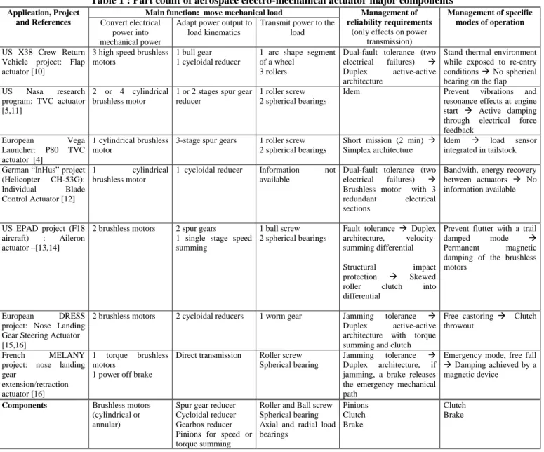
As contributors to the safety of embedded critical functions, aerospace actuators are subject to specific design requirements. In electromechanical PbW solutions, high reduction ratios between the motor and the load cannot be avoided in response to the low torque density of electric motors. Reliability requirements are usually met at the expense of multiple redundancies. Depending on the application, as the ultimate safety mode of operation, the load may have to be held in position (no motion), or its free motion may have to be damped. Based on recent examples [4-5, 10-16], Table 1 summarizes the main components that are involved in PbW aerospace actuators in response to these constraints. The last line of Table 1 points out the components that have been considered as sufficiently generic to make the development of dedicated estimation models worthwhile. The objective of these models is to provide tools that enable a quick evaluation of different actuator architectures during the preliminary design.

Table 1 : Part count of aerospace electro-mechanical actuator major components

Application, Project and References

Main function: move mechanical load Management of reliability requirements

(only effects on power transmission) Management of specific modes of operation Convert electrical power into mechanical power

Adapt power output to load kinematics

Transmit power to the load US X38 Crew Return

Vehicle project: Flap actuator [10]

3 high speed brushless motors

1 bull gear 1 cycloidal reducer

1 arc shape segment of a wheel

3 rollers

Dual-fault tolerance (two electrical failures)  Duplex active-active architecture

Stand thermal environment while exposed to re-entry conditions  No spherical bearing on the flap US Nasa research

program: TVC actuator [5,11]

2 or 4 cylindrical brushless motor

1 or 2 stages spur gear reducer

1 roller screw 2 spherical bearings

Idem Prevent vibrations and resonance effects at engine start  Active damping through electrical force feedback European Vega Launcher: P80 TVC actuator [4] 1 cylindrical brushless motor

3-stage spur gears 1 roller screw 2 spherical bearings

Short mission (2 min)  Simplex architecture

Idem  load sensor integrated in tailstock German “InHus” project

(Helicopter CH-53G): Individual Blade Control Actuator [12]

1 cylindrical brushless motor

1 cycloidal reducer Information not available

Dual-fault tolerance (two electrical failures)  Brushless motor with 3 redundant electrical sections

Bandwith, energy recovery between actuators  No information available

US EPAD project (F18 aircraft) : Aileron actuator –[13,14]

2 brushless motors 2 spur gears

1 single stage speed summing

1 ball screw 2 spherical bearings

Fault tolerance  Duplex architecture, velocity-summing differential Structural impact protection  Skewed roller clutch into differential

Prevent flutter with a trail damped mode  Permanent magnetic damping of the brushless motors

European DRESS project: Nose Landing Gear Steering Actuator [15,16]

2 brushless motors 2 cycloidal reducers 1 worm gear Jamming tolerance  Duplex active-active architecture with torque summing and clutch

Free castoring  Clutch throwout

French MELANY project: nose landing gear

extension/retraction actuator [16]

1 torque brushless motors

1 power off brake

Direct transmission Roller screw Spherical bearing

Jamming tolerance  Duplex architecture, if jamming, a brake releases the emergency mechanical path

Emergency mode, free fall  Damping achieved by a magnetic device

Components Brushless motors (cylindrical or annular)

Spur gear reducer Cycloidal reducer Gearbox reducer Pinions for speed or torque summing

Roller and Ball screw Spherical bearing Axial and radial load bearings Pinions Clutch Brake Clutch Brake

2.2. What parameters for the preliminary design?

The actuator design is driven by the following main aspects to meet the various requirements: integration (mass, geometrical envelope) between airframe and actuated load, resistance to environment (thermal and vibration) [17], instant power and energy saving, dynamic performance, service life, reliability, resistance to or tolerance of failures. When dealing with these various topics in a model-based way, the designer often fails to obtain the relevant parameters of the component models rapidly. In order to generate the estimation model from a reduced number of key data, we propose to categorize these parameters as follows:

- Integration parameters, required to evaluate the masses and major dimensions of the components.

- Simulation parameters, required for sizing from a dynamic simulation of the mission profile (e.g. inertia or moving mass, heat capacity, reducer compliance)

- Operating domain parameters, required to verify the component use with respect to e.g. service life or safe operating areas (SOA).

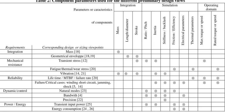
Table 2 is used to help the categorize component characteristics (columns) according to the multiple design tasks (lines), which are generally considered individually as illustrated by the bibliographical references. In the following sections, all the parameters listed in this table will be derived from key design parameters, called definition parameters here, to make the estimation model as versatile as possible.

Table 2: Component parameters used for the different preliminary design views

Parameters or caracteristics of components

Integration Simulation Operating domain M ass Le n g th /d ia m et er S tr o k e R at io / P it ch In er ti a S ti ff n ess / b ac k la sh F ri ct io n / Ef fi ci en cy El ec tr ic al p ar am et er s Th er m al p ar ame te rs M ax t o rq u e o r sp ee d R at ed t o rq u e o r sp ee d

Requirements Corresponding design or sizing viewpoints

Integration Mass [18]  Geometrical enveloppe [18,19]   Mechanical resistance Transient stress [12]     Fatigue/thermal/wear stress [20]    Vibration [14, 21]     

Reliability Life time / MTBF / failure rate [20]   

Failure/Critical cases: winding short circuit, jamming, shock [5, 14]

     

Dynamic/control Natural modes [23]    

Bandwith [4]    

Precision [22] 

Power / Energy Transient input power [25]    

Energy consumption [24 , 26]  

3. ESTIMATION MODELS FOR SYSTEM LEVEL DESIGN

3.1. Estimation models

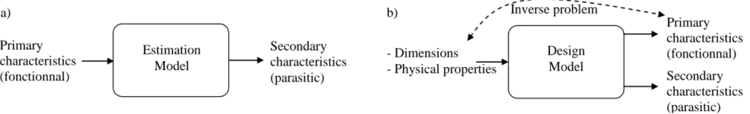
As described in Section 2.2, the system-level design steps require models (Figure 1a) directly linking primary characteristics, which define the component functionally, to secondary characteristics, which can be seen as the features of imperfections [28]. Generally, at component level, the models (Figure 1b) link the physical dimensions and characteristics of materials used to the primary and secondary characteristics. The design at component level is an inverse problem which requires the primary characteristics as inputs. This inversion may be done through design codes from design mechanical standards [22], by algebraic solvers or by optimization algorithms [27]. At system level, this approach requires very significant expertise for each component. It is therefore cumbersome to implement and shrinks the component range to a reduced number of candidate technologies.

A first direct approach consists of using databases as is done in some design software packages [29]. Its main disadvantage is that it is cumbersome or even impossible to implement in the absence of a product range as is the case in the aerospace field. Although it is interesting for optimization, data mining combined with response surface modelling (RSM) [30] seems inappropriate here for the same reason. The use of scaling laws, also called similarity laws or allometric models, has the advantage of requiring only one reference component for a complete estimation of a product range. Such a modelling approach has already been used with success for component design or comparison of technologies [31-35]. This approach is developed here for system level design with the components

defined in Section 2.1, since it appears to be the most appropriate means of speeding up the preliminary design of aerospace actuators. Estimation Model Primary characteristics (fonctionnal) Secondary characteristics (parasitic) Design Model - Dimensions - Physical properties Primary characteristics (fonctionnal) Secondary characteristics (parasitic) a) b) Inverse problem

Figure 1: Component models a) for system level design b) for component level design.

3.2. Main assumptions

Scaling laws study the effect of varying representative parameters of a component compared with a known reference. This article uses the notation proposed by M. Jufer in [31]. The x* scaling ratio of a given parameter is calculated as:

ref

x x

x*  (1)

where xref is the parameter taken as the reference and x is the parameter under study.

The scaling laws reduce the complexity of the inversion problem of Figure 1b by using two key modelling assumptions on the input parameters:

- All material properties are assumed to be identical to those of the component used for reference. All corresponding scaling ratios are thus equal to 1. For example E* = * = 1 with E* and * being respectively the variation of the Young’s modulus and density of the material;

- The ratio of all the lengths of the considered component to all the lengths of the reference component is constant. Used in range definition [37], this geometric similarity assumption leads to dimension scaling ratios that are all identical and equal to a dimension variation, noted l* here

Using scaling laws reduces the number of inputs, as shown in Figure 2a. It is then easy to express all the useful relations (see Section 2.2) as a function of a key design parameter that is associated with the component under design. We propose to call it the definition parameter, according to the layout of the proposed estimation model,

Figure 2b. The remainder of this paper will describe how to obtain these parameters by pointing out the main assumptions and the physical or design drivers that are at the origin of the relevant scaling law. The scaling laws supporting parameter estimation will be given as tables in Section 5.

S c a lin g la w m o d e l S c a lin g la w m o d e l fo r e stim atio n - D im e n sio n s * * * ... l d r    - P h ysic a l p ro p e rtie s 1 ... * *     E P rim a ry c h a ra cte ristic s (fu n c tio n al) S e c o n d a ry c h a ra cte ristic s (d e fe c ts) (fo n c tio n n al) se c o n d a ire s

a ) b )

D e fin itio n pa ra m e te r R a te d to rq ue T*

In te gra tio n p a ra m ete rs :

m a ss M*, d im e n sio ns d*= l*= …

S im u la tio n p a ram e te rs :

in ert ia J*, stiffn e ss K*, …

O p e ra tin g a re a s :

m a x to rq u e T*, m a x sp eed K*, …

Figure 2: Scaling laws models a) according to dimension variation b) according to definition parameter.

3.3. Direct effect of geometrical similarity on parameters

The parameters representing geometric quantities can be directly derived from the assumption of geometric similarity. For example, the variation of the volume V of a shaft (cylinder) of length l and radius r, in the case of identical variation for all geometrical dimensions (r*=l*) is:

3 * * 2 * 2 2 * l l r l r l r V V V ref ref ref       (2)

This result remains valid for any other geometry. In the same way, it is possible to calculate the variation of the mass, M, and rotational moment of inertia, J, of the shaft:

         





where ρm is the mass density of the shaft.

3.4. Different ways of finding the scaling laws

The scaling laws can be obtained in different ways. Three of them will be illustrated using the example of the thermal time constant of an electric motor. It is assumed here that the motor temperature rise is uniform and is mainly due to convection between the stator and the air (this assumption can be refined, cf. Section 5.2.1).

3.4.1. Direct approach

The first approach [31] directly uses the analytical expression for the quantity under study. The thermal time constant th can thus be expressed by:

th th

th  R .C



(4)

with Rth the thermal resistance and Cth the thermal capacity. As 2 * * / 1     hS R l R_{th th} (5)

with h the convection coefficient and S the thermal exchange surface and 3 * * . . M C l c C_th  _v   _th  (6)

with cv the thermal capacity density,  the density and M the motor mass the corresponding scaling law for the thermal time constant becomes:

* * l th   (7)

3.4.2. Dimensionless number approach

A second approach uses the dimensionless number obtained from the ratio of power or energy [37,38]. The dimensionless number corresponding to the present example, close to the Fourier number, is obtained as the ratio of the energy stored in a solid to the convective heat flux :

t h l cm . . convection of rate Energy solids in storage of rate Energy  (8)

with t a characteristic time for the phenomena. This number is constant for:

h l c t  m. (9) thus * * l th   (10)

3.4.3. Buckingham theorem approach

A third approach uses the Buckingham  theorem [39, 40] to obtain dimensionless  numbers. For our example, there is a relationship:





(1)

with d and l the diameter and the length of the motor. Using the Buckingham  theorem , this relationship becomes :

0 , _      d l h l c F th v   (11)

The assumption of geometric similarity reduces the π numbers to be considered. We thus find the relation:

0 ' _       th v h l c F   (12) thus te th v C h l c    (13) and finally * * l th   (14)

4. MAIN DESIGN DRIVERS FOR ELECTROMECHANICAL COMPONENTS

Product ranges are usually defined using the same material stresses and the same design drivers. The induced relations link the dimensions with the different parameters (definition, integration, simulation, operation area) associated with the components. This section summarizes these design drivers for electromechanical components and prepares the writing of estimation models of Section 5.

4.1. Mechanical design drivers

4.1.1. Mechanical stress

For mechanical components, the mechanical stresses in the materials must be kept below elastic, fatigue or contact pressure (Hertz) limits [41]. Taking the same stress limit  [37] for a full product range yields:

2 * * * 1 F l   (15)

The dimensional analysis enables the transmitted force F , or the transmitted torque T to be linked with geometrical dimension for a rotational component:

3 * * 2 * * l T l F    ₍₁₆₎

From the previous expression, the evolutions of the diameter, length, mass, inertia and all other parameters can be expressed as a function of the transmitted nominal force F* or torque evolution T*.

The ratio between fatigue stress and maximum stress is fixed for a given material. In the case of a reducer, the absolute torque that the reducer can transmit corresponds to the maximum stress it can withstand. Therefore the change in maximum peak torque Tmax is proportional to the change in nominal torque Tnom .

* * * max T T T  _nom  (17)

4.1.2. Stress-strain relationship effects

1

.   * * 

 E l l

 ₍₁₈₎

with E the Young’s modulus

This suggests that, for a given technology, a range of rotary components (e.g. gear reducers) has a constant backlash 1 * * *_{  }  l l ₍₁₉₎

and a stiffness that is proportional to the transmitted torque

* * * * T T K    ₍₂₀₎

4.1.3. Maximal speed of rotation

The maximal rotational speed ωmax of a mechanical component can be limited by mechanical constraints induced by centrifugal forces or by axial or transverse vibrations. At high speeds, rotating components, e.g. permanent magnets of brushless motors, run a risk of detachement due to centrifugal forces. Assuming all dimensions vary with the same ratio gives

2 * 2 * * .l centr    (21)

The resonance frequency f can be linked to density , Young’s modulus E and dimension l using a dimensional analysis: * * * * 1  E l f  (22)

With the assumptions*  E*  * 1, these two equations provide the same scaling law for maximal speed: 1 * max * _  l  ₍₂₃₎

4.2. Electromagnetic design drivers

The main design driver of electromagnetic devices concerns their magnetic and electrical circuits.

4.2.1. Magnetic circuit with permanent magnets

For a magnetic circuit including permanent magnets, such as those encountered in brushless motors, the magnetic field can be high even with a significant air gap. The flux density in the common iron sheet must not exceed given values in order to avoid saturation and corresponding associated losses. A range of electromagnetic components must be sized with a constant maximal flux density. Hence

1

* _

B ₍₂₄₎

For a magnetic circuit involving a magnet characterized by a remanent magnetization Br, a length Lm and an airgap of width e, the flux density can be expressed by the following relation [42]:

1 1 1 _ * _   B L e B B m r (25)

The assumption of geometric similarity induces a constant magnetic field for an entire range of products. The electromagnetic torque can therefore be deduced from the Laplace forces [35, 31]:

4 * * * 4 * * * l J B l J T JBrdv T 



4.2.2. Magnetic circuits without permanent magnets

For magnetic circuits without permanent magnets, such as those encountered in clutches and brakes, air gaps must be small in order to get large magnetic fields. The mechanical constraints described in the preceding paragraph must also be taken into account. Assuming homothetic variation and using the notations of Figure 3b, the flux density can be expressed by the following relation [42]:

* * * 0 1 1 l J B e A e JA B r iron co             (27)

The magnetic fields increase with machine size, which could lead to iron saturation. For small size magnetic circuits the electromagnetic force is expressed by:

4 * 2 * * 3 * * * l J B l J F   ₍₂₈₎ Permanent magnet Lm e Winding e Aco copper cross section area

Airon iron cross section area

Lm magnetic circuit length

Figure 3: Induction in magnetic circuit with a) permanent magnet b) coil.

4.2.3. Electrical circuits

Electrical circuits including windings should be designed to make their operating voltage compatible with the power source or the power electronics. This voltage is related to the number of coil turns n. An analysis of the back emf constant K enables to find n as a function of the operating voltage U:

* * 2 * * * * 2 * * * * *       B l U n B l n U K (29)

The number of turns is also involved in the expressions for winding resistance and inductance:

1 * 2 * * _  l n R ₍₃₀₎ * 2 * * l n L  ₍₃₁₎

4.3. Thermal design drivers

4.3.1. Temperature rise limits

Thermal stress is an important design driver for electromechanical components. The temperature rise of the winding insulation and of the lubricant of mechanical components must not exceed given temperatures if they are to operate correctly. The maximum temperature  should be constant throughout a range of products, giving:

1

* _

 ₍₃₂₎

For electromechanical components, the relationships between energy loss and temperature are established assuming a geometric similarity. Heat dissipation is essentially proportional to the convective surface area because

the materials involved, mainly metals, are good thermal conductors. The temperature gradients are essentially localized at the outer surfaces for convection with the surroundings or at the insulation of the coils for conduction (the insulation thickness is constant for a given voltage range). Therefore:

2 * * * 2 * * . P l l Ploss    loss  ₍₃₃₎

The design constraints induced depend on the nature of the losses encountered.

4.3.2. Electromagnetic losses

For brushless motors or electromagnetic devices; the Joule effect is the main source of losses at low speed :

3 * 2 * * , J l P_{loss Joules}  _el (34)

with Jel the surface current density.

With a fixed maximum admissible temperature, the nominal current density in the conductors is thus expressed by [31] : 2 1 * * _  l J_el (35)

The iron losses can become significant for higher speeds, especially in the brushless motors used in aerospace applications, with high speed or high torque and a large number of poles . Some brushless motors are thus not limited in speed by the centrifugal forces on the magnets but rather by the thermal constraints and iron losses. The losses of a motor are given mainly by the sum of the Joule losses PJ (copper) and iron losses, Piron:

iron J motor loss P P P _,   (36)

According to the Steinmetz-like formula provided in [43] the variation of the iron losses can be expressed as

* * * . _iron b iron f M P  (37)

where f is the electrical frequency and Miron is the iron mass.

Based on the work of G. Grellet [43], an average value of 1.5 can be considered for b. According to the thermal limit of the motor, the maximum iron losses Piron,ωmax that occur at the maximum speed (when not limited by the centrifugal constraint) are equal to the maximum admissible power losses since no electromagnetic torque causes Joule losses (see Figure 8). Thus, the evolution of the fmax maximum electrical frequency with respect to the thermal limit is:

b

l f_max*  *1

(38)

Taking into account of the number of pairs of poles, the maximum admissible speed of a motor with respect to its thermal limit can be expressed easily.

4.3.2. Mechanical losses

Other sources of loss are the frictional losses in mechanical parts. These losses increase with speed, causing the temperature to rise. Consequently, the lubricant becomes more fluid, with degraded bearing properties that increase the friction coefficient. Beyond a critical temperature, i.e. at maximum speed ωmax, this phenomenon causes unacceptable wear damage. This speed limit is common to many mechanical components, e.g. rolling bearings, which are also present in screws or reducers:

1 * * * max * * * * * * . . .    

 _{nom nom nom}

th F l F l F

5. EMACOMPONENT MODELS

This section describes estimation models for the electromechanical components of Table 1. The models are oriented to minimize entry definition parameters as proposed in Figure 2b. The bulk of the contribution of this section is contained in Table 3 to Table 7..

5.1. Mechanical components

5.1.1. Bearings and ball/roller screws

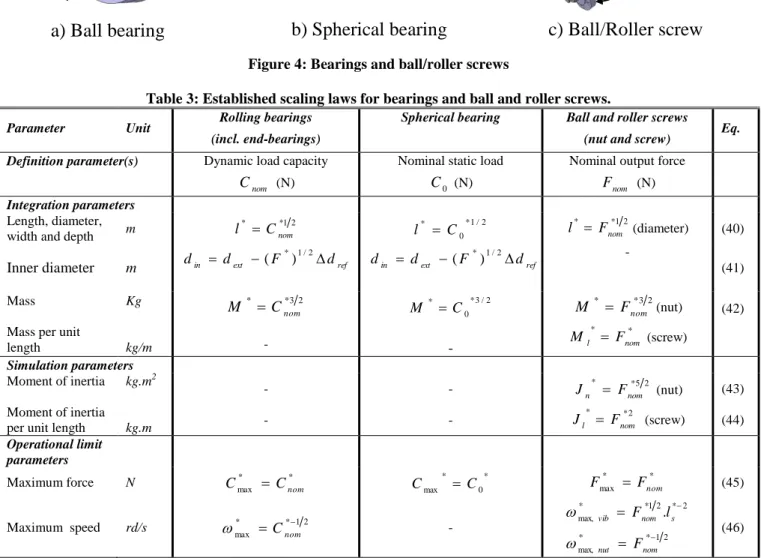
Bearings and ball/roller screws, Figure 4, are mainly modelled here assuming a constant admissible stress, as explained in section 4.1. Resulting scaling laws are given in Table 3.

screw

nut

end-bearing

a) Ball bearing

b) Spherical bearing

c) Ball/Roller screw

din

inclued rod-end

dext

l

Figure 4: Bearings and ball/roller screws

Table 3: Established scaling laws for bearings and ball and roller screws.

Parameter Unit Rolling bearings

(incl. end-bearings)

Spherical bearing Ball and roller screws

(nut and screw) Eq. Definition parameter(s) Dynamic load capacity

nom C (N)

Nominal static load 0

C (N)

Nominal output force nom

F (N)

Integration parameters

Length, diameter, width and depth m

2 1 * * nom C l  *1/2 0 * C l  l*  Fnom*12(diameter) (40)

Inner diameter m din  dext  F dref

2 / 1 * ) ( d_in  d_ext (F*)1/2d_ref - (41) Mass

Mass per unit length Kg kg/m 2 3 * * nom C M  - 2 / 3 * 0 * C M  - 2 3 * * nom F M  (nut) * * nom l F M  (screw) (42) Simulation parameters Moment of inertia Moment of inertia per unit length

kg.m2 kg.m - - - - 2 5 * * nom n F J  (nut) 2 * * nom l F J  (screw) (43) (44) Operational limit parameters Maximum force N * * max Cnom

C  C_max*  C₀* Fmax*  Fnom* (45)

Maximum speed rd/s * * 12 max  C_nom  - 2 1 * * max, 2 * 2 1 * * max, .     nom nut s nom vib F l F   (46)

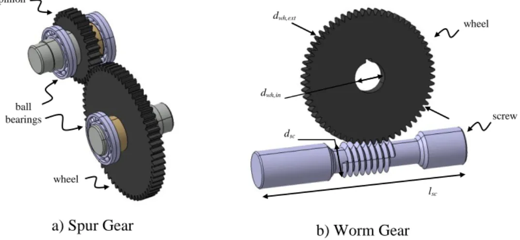
5.1.2. Gear assembly and worm reducer

Gear assemblies and worm gearings, Figure 5, are used to adapt the motor to the load impedance and also for power summation or power split. Force summation allows duplex power paths or geometric adaptation to the load (distance between centres, interface with load, countershaft ...). Their description, even at preliminary level, may therefore require geometric parameters to be used with increased attention. The assumption of geometric similarity is made here on the tooth or the screw thread which bears the mechanical stress.

By associating scaling law models, in particular for pinions and wheels as described in Table 4, a spur gear model can be built in agreement with the reduction ratio, the minimal number of pinion teeth and use of the same tooth module for pinion and wheel. In the same way a worm gear scaling law can be defined. The ball bearing model of the previous section can also be used to complete this reducer definition.

a) Spur Gear _{b) Worm Gear} pinion wheel ball bearings dsc dwh,ext lsc screw wheel dwh,in

Figure 5: Gear assembly and worm gear reducers

Table 4: Established scaling laws for gear assembly and worm gear reducers

Parameter Unit Pinion or Wheel Eq. Worm Gear Eq.

Definition parameter(s) Nominal torque nom

T (Nm) Number of teeth

Z

Nominal output (wheel) torque wh

T (Nm) Internal wheel diameter

in wh

d _,

(m)

Integration parameters

Tooth module M m* T_nom*1/3.Z*1/3 (47) Diameter M 3 / 2 * 3 / 1 * * * * . .Z T Z m d   _nom (48) * * *2/3 ,ext Δ wh wh wh d T d  (49) Width M b*  m* T_nom*1/3.Z*1/3 (50) 3 1 * * * wh sc wh d T l   * , * ext wh sc d l  (51) Mass Kg M*  d*2b* T_nom* .Z* (52) * * wh wg T M  (53) Simulation parameters Moment of inertia kg.m2 3 / 7 * 3 / 5 * * 4 * * .Z T b d J   _nom (54) * *53 wh wg T J  (55) Operational limit parameters

Maximum torque N.m T_max* T_nom* (56) T_wh,max* T_wh,nom* (57) Maximum speed rd/s _max* _max,* _bearing (58) _max* _max,* _sc (59)

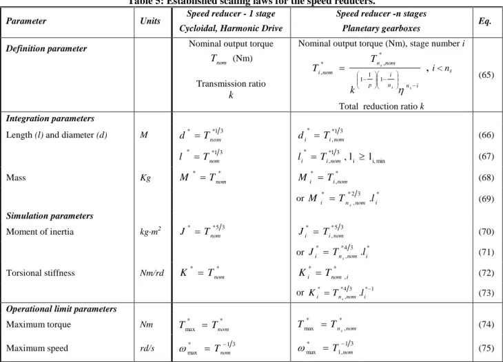
5.1.3. Reducers and gearboxes

The estimation models of can be used for planetary gear, harmonic drive [44] or cycloid drive reducers [45] (Figure 6). Unlike harmonic and cycloid drives, planetary gearboxes involve multiple gear stages to provide high reduction ratios. Therefore, Table 5 distinguishes single-stage (or first stage) and multiple-stage reducers. Once again, the main modelling assumptions are the geometric similarity (section 3.3) and the range sizing at constant admissible stress (section 4.1).

For planetary (epicycloidal) gearboxes, the manufacturers’ data show that each stage can reach a fixed maximum reduction ratio, ki,max (e.g. 10 for the planetary gearings in [46]) due to geometrical interference. The overall reduction ratio k is assumed to be shared equally between the ns stages here (ki=k

1/ns

). On the one hand, the last stage (i=ns, low speed shaft) is sized with respect to the torque to be transmitted. The scaling laws developed previously respect this requirement and therefore are applied to the last stage without changes. On the other hand, the torques transmitted by the supplemental stages are significantly reduced. Their sizing is not only driven by the transmitted torque but also by fatigue phenomena. Therefore, these stages are sized to match the lifetime of the last stage with respect to fatigue. The lifetime and the associated cumulated damages Qh, of a gearing with respect to fatigue is a function of its nominal torque and nominal speed, ωnom [47]:

nom p nom

h T

Q  . (60)

where p is an experimental constant that is equal to 10/3 or 3 depending on the bearing technology.

Equalizing the cumulated damages of the ith stage of reduction (for i < ns) with that of the last stage by considering the transmission ratio and mechanical efficiency of each stage gives

1 1 1 * , * , i n n i p nom n nom i s s s k T T                  (61)

where Ti,nom is the nominal torque of the i

th

stage. It should be noted that the fatigue constraint in the supplemental stages may be superseded by manufacturing or thermal constraints. There results a minimum length,

lmin, for a reduction stage. The total length of the planetary gear train is the sum of the stage lengths:



A detailed analysis of manufacturers’ catalogues shows two tendencies: the first one (68) where geometrical similarity is used for each stage, the second one (69) where, to rationalize production, outer diameters of the supplemental stages are imposed, identical to the last one in general. The total mass of the reducer is the sum of the stages masses.

In the same way, the inertia, Ji, of the i

th

supplemental stage is given by equation (70) or (71). The total equivalent inertia, Jeq, at the high speed shaft is the sum of the stage equivalent inertias, with a reduction equally shared among the stages:



The torsional stiffness, Ki, of the i

th

supplemental stage is given by equation (72) or (73). The total equivalent stiffness Keq at the low speed shaft is the combination of the different stage equivalent stiffnesses Ki,eq:

1 1 1 ,    _      



The mechanical limit to the maximum torque is given by the last stage of reduction, where this constraint is maximized. On the other hand, the limit to the maximum speed of the assembly is given by the first stage that has the smallest conductive surface area and the highest rotational velocity. Therefore the expressions for the maximum peak torque (74) of the maximum admissible speed (75) are applied to the last and first stages respectively.

Table 5: Established scaling laws for the speed reducers.

Parameter Units Speed reducer - 1 stage

Cycloidal, Harmonic Drive

Speed reducer -n stages

Planetary gearboxes Eq.

Definition parameter Nominal output torque

nom T (Nm)

Transmission ratio

k

Nominal output torque (Nm), stage number i

1 1 1 * , * , i n n i p nom n nom i s s s k T T                 

,

Total reduction ratio k

(65)

Integration parameters

Length (l) and diameter (d) M * *13

nom T d  d_i* T_i*_,1_nom3 (66) 3 1 * * nom T l  l_i*  T_i,*1_nom3 ,l_i  l_i,min (67)

Mass Kg M * T_nom* M_i*  T_i,*_nom (68)

or *23 * , * ._i nom n i T l M s  (69) Simulation parameters

Moment of inertia kg·m2 J* T_nom*53 J_i* T_i*_,nom53 (70) or J_i* T_n*4_,nom3 .l_i*

s

 (71)

Torsional stiffness Nm/rd K*  T_nom* K_i* T_nom* _,i (72) or K_i*T_n*4_,nom3 .l_i*1

s (73)

Operational limit parameters

Maximum torque Nm * * max Tnom T  *, * max Tn_s nom T  (74) Maximum speed rd/s * 13 max  T_nom  13 , 1 * max  T _nom  (75) 5.2. Electromechanical components 5.2.1. Brushless motors

The permanent magnet brushless motor can have two different geometrical configurations:

- Cylindrical (Figure 7a) with a constant number of poles and homothetic variation of all the dimensions; - Annular (Figure 7b) with an increasing number of poles and a constant ring thickness e, for an increasing

radial dimension.

a) Cylindrical b) Annular

Figure 7: Brushless motors (based on [35])

For both types of motors, the estimation models can be obtained under the same main assumption of a constant magnetic field, as described in section 4.2. However, the assumptions of geometric similarity differ and generate

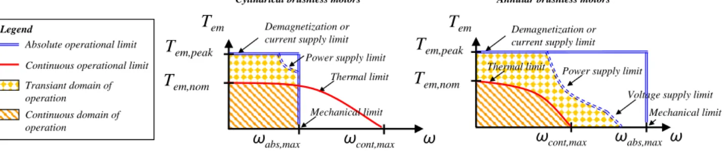
Table 6. Depending on the type of motor, the typical operational areas can also be different. As shown in Figure 8, it can be interesting to distinguish the speed limit from original mechanical constraints (section 4.1) abs, max from

those of thermal origin (section 4.3) cont, max. In the latter case, it is important to take into account the general trend

of losses. As explained in section 4.3, the Joule (or copper) losses are proportional to the square of the electromagnetic torque, while the iron losses, as given in [43], are a function of the electrical frequency, i.e. the angular velocity:      J Piron b rotor P em motor loss T P _, . 2  . ( 76 )

where the coefficients α and β are the Joule and iron loss coefficients respectively.

The estimated iron losses are also of importance when their damping effect (negative slope in torque/speed characteristic) is used to avoid flutter [12]. This loss model can be connected to one- or two-body thermal models (distinguishing the copper temperature from the iron temperature or not) [36] where the thermal resistances are proportional to the surface area and the thermal capacitances are proportional to the mass.

Tem ω Tem,nom ω_cont,max T_em,peak ω_abs,max Thermal limit Absolute operational limit

Continuous operational limit

Mechanical limit Power supply limit

T_em ω Tem,nom ω_cont,max T_em,peak ω_abs,max Demagnetization or current supply limit

Thermal limit Power supply limit

Mechanical limit

Demagnetization or current supply limit

Voltage supply limit

Legend

Cylindrical brushless motors Annular brushless motors

Transiant domain of operation

Continuous domain of operation

Table 6: Established scaling laws for brushless motors

Parameter Units Cylindrical motor Annular motor Eq.

Definition parameter

Nominal continuous torque Nm T_em* _,nom l*3.5 T_em*_,nom l*3 (77)

Operating voltage V * * * l n U  * ,max 3 * * * elec l n U   (78) Integration parameters

Length and diameter m l* T_em*1_,3_nom.5 l*  T_em*1_,3_nom (79) Mass kg M * T_em*3_,nom3.5 M * T_em*2_,nom3 (80)

Simulation parameters

Moment of inertia kg·m2 J* T_em*5_,nom3.5 J* T_em*4_,nom3 (81) Joule loss coefficient W/(Nm)2 * 53.5

, * _  nom em T  * 43 , * _  nom em T  (82)

Iron loss coefficient W/(rd/s)b *  T_em*3_,nom3.5 3 2 * , * b nom em T    (83)

Thermal resistance(s) K/W R_th*  T_em*_,2_nom3.5 R_th* T_em*_,2_nom3 (84) Thermal capacitance(s) J/K C_th*  T_em*3_,nom3.5 C_th*  T_em*2_,nom3 (85) Thermal time constant(s) S _th*  T_em*1_,nom3.5 _th* 1 (86) Torque or emf constant N/A or

V/(rad/s) 5 . 3 1 * , * * nom em T U K  * , 3 * * * nom em T l n K   (87)

Electrical resistances  R* U*2T_em*_,3_nom3.5 *2/3 , 2 * 2 * * nom em T l n R   (88)

Electrical inductances H L* U*2T_em*_,1_nom3.5

3 / 2 * , 2 * 2 * * nom em T l n L   if n*=1 (89)

Operational limit parameters

Absolute maximum torque Nm T_em* _,peak  T_em* _,nom

* max , * ,peak em em T T  (90)

Absolute maximum speed (mechanical limit)

Maximum speed (electrical limit)

rd/s _abs* _,max T_em*_,1_nom3.5

3 1 * , * max ,   _emnom abs T  1 = if 1 * , * 3 * 1 * * * max , * nom em elec n T U l n U       (91)

Continuous maximum speed (thermal limit) rd/s cont Temnomb    3.5 1 * , * max ,  *,13 * max ,   _{em nom} cont T  (92)

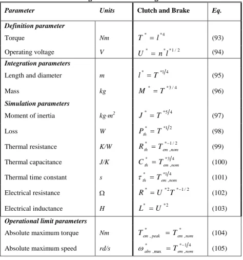
5.2.2. Electromagnetic clutches and brakes

The dimensions of electromagnetic clutches and brakes are mainly related to those of their electromagnet. The design criteria are therefore those described in section 4.2.3.

Table 7: Established scaling laws for electromagnetic clutches and brakes

Parameter Units Clutch and Brake Eq.

Definition parameter Torque Nm T* l*4 (93) Operating voltage V * * *1/2 l n U  (94) Integration parameters

Length and diameter m l* T*14 (95)

Mass kg M * T*3/4 (96)

Simulation parameters

Moment of inertia kg·m2 J* T*54 (97)

Loss W P_th* T*12 (98)

Thermal resistance K/W R_th* T_em*1_,nom/2 (99) Thermal capacitance J/K C_th* T_em*3_,nom4 (100) Thermal time constant s _th* T_em*1_,4_nom (101) Electrical resistance  R* U*2T*1/2 (102) Electrical inductance H L* U*2 (103)

Operational limit parameters

Absolute maximum torque Nm T_em* _,peak  T_em*_,nom (104) Absolute maximum speed rd/s _abs* _,max T_em*_,1_nom4 (105)

5.3. Validation of estimation models

Unlike the similarity laws obtained statistically [28], the form and the exponents of the relations established in section 5 were justified by the physical considerations of section 4. These scaling laws have been compared with manufacturing company data [44-46,48,49] for validation. The proposed equations remain valid for extrapolating the performance of a single component. Erreur ! Source du renvoi introuvable.a to Erreur ! Source du renvoi introuvable.c illustrate the interest of the estimation models for motors and reducers. The good agreement is also confirmed for other components. Log-log graphs have the advantage of covering a large definition range by giving straight lines as a result of the analytical form of the scaling laws. The slope of the log / log graph is given by the exponent of the power law while the selected reference product fixes a particular point of this curve:

) log( . log ) log( * * x b x y y x x y y x y _b ref ref b b ref ref b _              ( 106 )

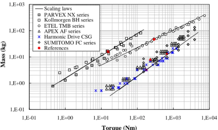
Erreur ! Source du renvoi introuvable.a to Erreur ! Source du renvoi introuvable.c validate the scaling laws established for mass, inertia and maximal speed estimations. In the context of technology selection, it can be seen in Erreur ! Source du renvoi introuvable.a that all the three types of reducers studied have comparable torque/mass ratios, although the harmonic drives show the best characteristics, followed closely by the cycloid reducer. Motor data are plotted for framed cylindrical motors as well as frameless annular motors. The latter therefore have an advantage with respect to mass considerations, partly for their hollow rotor shaft and absence of rotational bearings.

Erreur ! Source du renvoi introuvable.a shows that the scaling laws established for the motors’ thermal simulation parameters provide an efficient estimation of the effective values given by the manufacturer. The dispersion observed for annular motors comes from the non-homothetic scaling of the whole product range as designed by the manufacturer according to his catalogue. Different lengths of motors are proposed for a given diameter, allowing easy derivation of a given design to obtain an extended range. This is one limitation of the estimation models developed on the basis of the geometrical similarity principle.

Erreur ! Source du renvoi introuvable.c globally confirms the capability of scaling laws to estimate the maximal admissible speed. However, the maximum losses of annular torque motors do not differ significantly from the estimated value for definition torques below 40 Nm. Analysing the manufacturers’ data shows that these motors become limited by the maximal input voltage. The design driver used to establish the scaling laws is no longer applicable. The speed limit evolution for a fixed maximum input voltage (here 600 VDC) has been represented by a dashed line in Erreur ! Source du renvoi introuvable.c. This input voltage constraint can be explained by the rationalization of the power electronics product range associated with the motors. In this sense, the established scaling law provides the maximum speeds that the motors could reach without restriction on power electronics.

(a) Brushless motor and speed reducer masses as a function of the nominal torque.

(b) Brushless motor and speed reducer moment of inertia as a function of the nominal torque.

(c) Maximum speed as a function of the nominal torque.

Figure 9: Mass, inertia and speed as a function of the nominal torque for brushless motors and reducers

1,E+00 1,E+01 1,E+02 1,E+03 1,E+04

1,E-01 1,E+00 1,E+01 1,E+02 1,E+03 1,E+04

Torque (Nm) M a x imu m sp ee d ( rd /s) Scaling laws PARVEX NX series Kollmorgen BH series ETEL TMB series APEX FA series Harmonic Drive CSG series SUMITOMO FC series References Fixed maximum input voltage 1,E-07 1,E-06 1,E-05 1,E-04 1,E-03 1,E-02 1,E-01 1,E+00 1,E+01 1,E+02

1,E-01 1,E+00 1,E+01 1,E+02 1,E+03 1,E+04

Torque (Nm) M o m en t o f in er ti a ( k g .m²) Scaling laws ETEL TMB series Kollmorgen BH series PARVEX NX series APEX AF series Harmonic Drive CSG series SUMITOMO FC series References 1,E-01 1,E+00 1,E+01 1,E+02 1,E+03

1,E-01 1,E+00 1,E+01 1,E+02 1,E+03 1,E+04

Torque (Nm) M a ss (k g ) Scaling laws PARVEX NX series Kollmorgen BH series ETEL TMB series APEX AF series Harmonic Drive CSG SUMITOMO FC series References

The predictive significance of the scaling laws of Table 4 can be observed in Figure 10, which plots the manufacturing company’s data [50-53] versus what is predicted from the estimation model. Figure 10 shows that points representative of mass and inertia of gear and worm pinions fall closely around a straight line of slope one with a standard deviation for the error of these models of less than 10 %. Estimation models for other components such as ball bearings and roller screws are validated in [54].

0,01 0,10 1,00 10,00 100,00 1000,00 10000,00 0,01 0,10 1,00 10,00 100,00 1000,00 10000,00 M_catalog (kg) M_ scaling ( kg ) Redex Andantex QTC-Gears reference WormGear DYNABOX WormGear CAVEX K88 error max = 30% standard deviation = 7,6%

(a) Pinion masses for spur and worm gear

1,E-07 1,E-06 1,E-05 1,E-04 1,E-03 1,E-02 1,E-01 1,E+00

1,E-07 1,E-06 1,E-05 1,E-04 1,E-03 1,E-02 1,E-01 1,E+00

J_catalog (kg.m²) J_ scaling ( kg.m²) Redex-Andantex QTC-Gear reference WormGear DYNABOX WormGear CAVEX K88 error max = 38% standard deviation = 9,5%

(b) Pinion inertia for spur and worm gear

Figure 10: Mass and inertia of pinions and wheel in gear and worm reducers

6. FURTHER APPLICATIONS OF THE ESTIMATION MODELS

The objective of the paper is to provide enabling tools for the pre-design, simulation or optimization tasks. The proposed estimation models associated with other system simulations, CAD, reliability and optimization models support the preliminary design efficiently, where only a few design parameters are available but major technical decisions are to be taken:

- Their use with system simulation models and inverse simulation enable quick sizing and architecture evaluation even with complex mission cycles. Refs. [54, 55,18,56] give examples of the implementation of such CAE tools in the Modelica language [57] dealing with examples of an aileron, a spoiler or nose landing gear steering actuators.

- Their connection with CAD software can improve and accelerate the integration study. Ref. [19] gives an example of a geometrical integration study in the CATIA framework for a nose landing gear door actuator.

- Their uses with degradation models enable lifetime and reliability to be assessed. Thus [58] deals with the design for reliability of electromechanical actuators.

- Their use in the design of experiments and optimization algorithms enables optimal design of electromechanical actuators. Ref. [59] is an example of optimal geometrical integration of a linear actuator with a minimal mass objective.

7. CONCLUSION

A technology shift towards more electric solutions is emerging in aerospace actuation. New technology brings new challenges, especially for the preliminary design process of actuation systems and components that cannot simply be a duplicate of former practices. In this way, it is no longer meaningful to proceed to sizing by points (as for hydraulic actuators). Instead, it is necessary to take into account mission profiles covering all possible sizing drivers (e.g. maximum speed and torque, fatigue, thermal behaviour, vibrations and shocks) and addressing various design criteria (e.g. geometrical envelope, weight and reliability). For this purpose, appropriate top level evaluation tools should be developed to support an efficient preliminary design. In this paper, such tools have been proposed in the form of models for the major generic EMA components, which are first identified by a state-of-the-art of the actuation systems in aerospace and aeronautics. This state-of-the-art also highlights the different stages or design points of view encountered in early preliminary studies. Then a classification of the design parameters associated with these stages has been proposed to fit into a model-based design approach. Obtaining these parameters quickly and easily is a critical issue for sizing calculations and early simulations in the framework of risk mitigation. The scaling law approach presented in this paper responds to this issue by allowing the development of component models from a limited number of input parameters. Moreover, the scaling laws developed are representative of the state-of-the-art of technology and require a single component reference instead of a large amount of data that is cumbersome to set-up and maintain. These laws have been compared with manufacturers’ catalogue data to validate their relevance. Finally, the usefulness of these estimation models has been illustrated with potential applications for EMA model based designs.

8. ACKNOWLEDGMENTS

The work presented was partly funded by the following projects: the FP6 European DRESS project (Distributed and Redundant Electro-mechanical nose gear Steering System, 2006/2009) and the French FUI CISACS project (Concept Innovant de Systèmes d’Actionnement de Commandes de vol secondaires et de Servitudes).

REFERENCES

1 T. Ford, "More-electric aircraft," Aircraft Engineering and Aerospace Technology, vol. 77, 02-2005 2005.

2 D. Van den Bossche, “A380 primary flight control actuation system”, International Conference on Recent Advances in Aerospace Actuation Systems and Components, June 13-15, 2001- Toulouse, p 1-4.

3 M. Todeschi, “Airbus – EMAs for flight actuation systems – perspectives”, International Conference on Recent Advances in Aerospace Actuation Systems and Components, June 13-15, 2010- Toulouse, p 1-8.

4 G. Dée, T. Vanthuyne, P. Alexandre, “An electrical thrust vector control system with dynamic force feedback”, International Conference on Recent Advances in Aerospace Actuation Systems and Components, June 13-15, 2010- Toulouse, p 75-79.

5 J. R. Cowan, R. A. Weir, “Design and test of electromechanical actuators for thrust vector control”, in NASA. Ames Research Center, The 27th Aerospace Mechanisms Symposium p 349-366, 1992.

6 Design methodology for mechatronic systems VDI-Richtlinien. Düsseldorf, VDI

7 INCOSE, Systems engineering handbook, INCOSE Technical Product, 2004.

8 J. A. Estefan, “Survey of Model-Based Systems Engineering (MBSE)”, INCOSE MBSE Focus Group, May 2007.

9 L. Han, C. J. J. Paredis, and P. K. Khosla, "Object-Oriented Libraries of Physical Components in Simulation and Design", in 2001 Summer Computer Simulation Conference, Orlando, FL, 2001, pp. 1-8.

10 J. Hagen, L. Moore, J. Estes, Ch. Layer, ”The X-38 V-201 Flap Actuator Mechanism”, Proceedings of the 37th Aerospace Mechanisms Symposium, Johnson Space Center, May 19-21, 2004.

11 D. E. Schinstock, D. A. Scott, “Controller Design for EMA in TVC Incorporating Force Feedback”, NASA/MSFC Technical Report, 1998.

12 D. Fuerst, T. Neuheuser, “Development, prototype production and testing of an electromechanical actuator for a swashplateless primary and individual helicopter blade control system”, 1st international workshop on aircraft system technologies (AST 2007), March 29-30, 2007, Hamburg, Germany, p 7-19.

13 S. C. Jensen, G. D. Jenney, D. Dawson, “Flight test experience with an electromechanical actuator on the f-18 systems research aircraft”, The 19th Digital Avionics Systems Conferences, Philadelphia, PA , USA, 07 Oct. 2000 - 13 Oct. 2000.

14 D. J. Kopala, Ch. Doel, “High Performance Electromechanical Actuation for Primary Flight Surfaces (EPAD Program Results)”, Recent Advances in Aerospace Actuation Systems and Components, June 13-15, 2001, Toulouse, France. 15 Liscouët, J., Orieux, S., & Maré, J.C., “An innovative top-down approach for the preliminary design of

electromechanical actuators”, Proceedings of the 26th International Conference on Aerospace Sciences, Anchorage, September 14-19, 2008.

16 P-Y. Chevalier, S. Grac, P-Y. Liegois, “More electrical landing gear actuation systems”, Recent Advances in Aerospace Actuation Systems and Components, May 5-7, 2010, Toulouse, France.

17 DOE 160 , “Environmental Conditions and Test Procedures For Airborne Equipment”, standard for environmental test of avionics hardware published by RTCA Incorporated. , March 2005.

18 F. Hospital, M. Budinger, J. Liscouet, J-Ch Maré, “Model Based Methodologies for the Assessment of More Electric Flight Control Actuators“, 13th AIAA/ATIO Aviation Technology, Integration and Operation Conference, 13 - 15 Sep 2010 - Fort Worth, Texas.

19 M. Budinger, A. Fraj, T. El Halabi, J-Ch. Maré, “Coupling CAD and system simulation framework for the

preliminary design of electromechanical actuators”, IDMME Virtual Concept, 20-22 October 2010, Bordeaux, France. 20 J. Liscouët, M. Budinger, and J.-Ch. Maré, “Design for Reliability of Electromechanical Actuators”, Recent Advances

in Aerospace Actuation Systems and Components, May 5-7 2010, Toulouse, France

21 S. Grand, J-M. Valembois, Electromechanical actuators design for thrust vector control, Recent Advances in Aerospace Actuation Systems and Components, November 24-26, 2004, Toulouse, France.

22 F. Roos, "Towards a methodology for integrated design of mechatronic servo systems”, KTH, Machine Design, 2007, pp. viii-203.

23 O. Cochoy, S. Hankea, U. B. Carla, Concepts for position and load control for hybrid actuation in primary flight controls, Aerospace Science and Technology, Volume 11, Issues 2-3, March-April 2007, Pages 194-201

24 J.Ch. Maré, M. Budinger, “Comparative analysis of energy losses in servo-hydraulic, hydrostatic and electro-mechanical actuators”, The 11th Scandinavian International Conference on Fluid Power, SICFP’09, Linköping, Sweden, June 2-4, 2009.

25 S. Girinon, C. Baumann, H. Piquet, N. Roux, Analytical modeling of the input admittance of an electric drive for stability analysis purposes, Eur. Phys. J. Appl. Phys. 47, 11101 (2009)

26 S. Liscouët-Hanke, S. Pufe, J-C. Maré, “A Simulation Framework for Aircraft Power Management”, Proceedings of the Institution of Mechanical Engineers, Part G: Journal of Aerospace Engineering, Volume 222, Number 6 / 2008, Pages 749-756..

27 F. Messine, B. Nogarede, and J-L. Lagouanelle, Optimal Design of Electromechanical Actuators: A New Method Based on Global Optimization, IEEE transactions on magnetics, vol. 34, no. 1, January 1998.

28 P. Krus, “Performance Estimation Using Similarity Models and Design Information Entropy”, Workshop on Performance Prediction in System-Level Design, International Design Engineering Technical Conference and Computers and Information in Engineering Conference (IDETC/CIE) , Aug. 3 2008.

29 ControlEng, ServoSoft software, www.controleng.ca.

30 T. Simpson, J. Peplinski, P. Koch and J. Allen, “Metamodels for Computer-Based Engineering Design: Survey and Recommendations”, Engineering with Computers, Vol. 17, pp. 129-150, 2001.

31 M. Jufer, "Design and Losses - Scaling Law Approach", in Nordic Research Symposium Energy Efficient Electric Motors and Drives, Skagen, Denmark, 1996, pp. 21-25.

32 G. Ricci, "Mass and rated characteristics of planetary gear reduction units," Meccanica, vol. 27, pp. 35-45, 1992. 33 G. Ricci, "Weight and rated characteristics of machines: positive displacement pumps, motors and gear sets",

Mechanism and Machine Theory, vol. 18, 1983, pp. 1-6.

34 K. J. Waldron, Ch. Hubert, “Scaling of robotic mechanisms”, IEEE International Conference on Robotics & Automation, San Francisco, CA, April 2000.

35 B. Multon, H. Ben Ahmed, M. Ruellan, and G. Robin, "Comparaison du couple massique de diverses architectures de machines tournantes synchrones à aimants", Société de l'Electricité, de l'Electronique et des Technologies de

l'Information et de la Communication (SEE), pp. 85-93, 2006.

36 D. Iles-Klumpner, I. Serban, M. Risticevic, I. Boldea, “Comprehensive Experimental Analysis of the IPMSM for Automotive Applications, Power Electronics and Motion Control Conference”, 2006. EPE-PEMC 2006. 12th International, Aug. 30 2006-Sept. 1 2006, Portoroz, pp. 1776 – 1783.

37 G. Pahl, W. Beitz, L. Blessing, J. Feldhusen, K.-H. Grote, and K. Wallace, “Engineering Design: A Systematic Approach”, London: Springer-Verlag London Limited, 2007.

38 Stephen J. Kline, “Similitude and Approximation theory”, McGraw-Hill Book Company, 1965. 39 E. S. Taylor, “Dimensional Analysis for Engineers”, Oxford University Press, 1974.

40 Glenn Murphy, “Similitude in engineering”, The Ronald press company. New York, 1950.

41 R. Budynas and J. K. Nisbett, “Shigley's Mechanical Engineering Design, SI version”. New York: McGraw-Hill, 2007.

42 A.E. Fitzgerald, Ch. Kingsley, S. D. Umans, “Electric Machinery”, Fifth Edition, McGraw-Hill Book Company, 1992.

43 G. Grellet, "Pertes dans les machines tournantes," Techniques de l'Ingénieur, 1989.

44 "Units CSG-2UH Digital Catalogue", Harmonic Drive, 2005, http://www.harmonicdrive.net/.

45 "Fine Cyclo Catalogue", Sumitomo Drive Technologies, 2005, http://www.sumitomodriveeurope.com/. 46 "AF Series Catalogue", APEX Dynamics Inc., 2009, http://www.apexdyna.com/.

48 "Synchronous Servomotors Series GOLDLINE™ BH, Technical description, Installation, Commissioning," Kollmorgen, 2000, http://www.kollmorgen.com/.

49 "Torque Motors Data Sheets, TMB Series," ETEL Motion technology, 2007, http://www.etel.ch/. 50 Modular rack&pinion system, www.andantex.com.

51 Quality Transmission Components, www.qtcgears.com,

52 CAVEX - Worm Gear Units, F. D. a. Automation, 2005. http://flender.com

53 Dynabox - Right angle servo gearheads, G. T.-P. gearheads, 2008, www.girard-transmissions.com.

54 J. Liscouët, M. Budinger , J-Ch. Maré, S. Orieux, Modelling approach for the simulation-based preliminary design of power Transmissions, accepted for publication in Mechanism and Machine Theory.

55 L. Allain, M. Budinger, J. Liscouet, Y. Lefevre, J. Fontchastagner, A. Abdenour, Preliminary Design of

Electromechanical Actuators with Modelica, Modelica 2009, Proceedings 7th Modelica Conference, Como, Italy, Sep. 20-22, 2009.

56 Budinger M., Liscouët J., Cong. Y.., Mare J-Ch., Simulation Based Design of Electromechanical Actuators with Modelica, IDETC 09, San Diego, 30 August, 2 September 2009.

57 S. E. Mattsson, H. Elmqvist, M. Otter, “Physical system modeling with Modelica”, Control Engineering Practice 6 (1998) pp 501-510.

58 J. Liscouët, M. Budinger, and J.-C. Maré, “Design for Reliability of Electromechanical Actuators”, Recent Advances in Aerospace Actuation Systems and Components, May 5-7 2010, Toulouse, France.

59 T. El Halabi, M. Budinger and J.-C. Maré, “Optimal geometrical integration of electromechanical actuators”, Recent Advances in Aerospace Actuation Systems and Components, May 5-7 2010, Toulouse, France.