A Study on the Deformation Behaviour of the Cathode Collector
Bar at High Temperature and Low Stress Levels
Mémoire
Femi Richard Fakoya
Maîtrise en génie civil
Maître ès sciences (M.Sc)
Québec, Canada
iii
Résumé
L'étude de la déformation de la barre collectrice dans les conditions subies au sein de la cellule de réduction d'aluminium est d'une grande importance pour l'optimisation de l'efficacité et l'augmentation de la durée de vie de la cellule. Ce mémoire nous informe des résultats d'un programme expérimental réalisé sur une barre de collectrice en acier. Le but, est d' étudier son comportement en tenant compte de ses propriétés thermiques, mécaniques et de fluage. Des essais ont été effectués en compression à de basses tensions, de 0,5 à 2MPa et à une température élevée, de 900°C. Différents comportements ont été observés à de faibles contraintes, jusqu'à 2MPa, cela peut être justifié par le temps et le niveau de pression appliqué. L'inspection métallographique a montré l'apparition d'oxydation et de la corrosion sur des échantillons testés, ceci est dû à l'environnement agressif des conditions du test. D'importants efforts et modifications ont été fournis pour éradiquer cet effet et pour améliorer l'exactitude des données de test de fluage obtenus.
v
Abstract
The study of the deformation behaviour of the collector bar at conditions experienced within the aluminium reduction cell is of great importance to optimizing the efficiency and increasing the life span of the cell. This mémoire communicates the results of an experimental program carried out on the steel collector bar material (AISI 1006) to investigate its behaviour in relation to its thermal, mechanical and the creep properties. Tests were carried out in compression at low stresses, 0.5 to 2 MPa and high temperature, 900 °C. Different behaviour was observed at low stresses up to 2 MPa, which can be characterised by time and applied stress level. Metallographic inspection showed effect of oxidation and corrosion on tested samples due to the aggressive environment of the test condition, major efforts and modification were made to eradicate this effect and to improve the accuracy of obtained creep test data.
vii
Table of Contents
Résumé ... iii
Abstract ... v
Table of Contents ... vii
List of Figures ... xi
List of Tables ... xv
Acknowledgement ... xvii
1. Introduction ... 1
1.1. Basics of aluminium production ... 1
1.2. Breakdown concept of aluminium production ... 2
1.2.1. Hall-Héroult cell ... 2
1.2.2. The cathode assembly ... 3
1.2.3. The steel collector bar ... 4
1.3. Problem ... 4
1.3.1. Introduction ... 4
1.3.2. Failure mechanism in the cathode assembly ... 4
1.3.3. Deformation of the steel collector bar ... 5
1.4. Deformation behaviour and properties of metals ... 7
1.4.1. Thermal properties ... 7
1.4.2. Mechanical properties - stress – strain – time relationships ... 7
1.5. Scope of work - objectives ... 10
1.6. Structure of thesis content ... 11
2. Literature Review ... 13
2.1. Background ... 13
2.2. Material Properties at High Temperature ... 13
2.2.1. Introduction ... 13
2.2.2. Effect of carbon content on material properties ... 13
2.2.3. Thermal properties ... 14
2.2.5. Creep properties ... 17
2.3. The phenomenon of creep ... 18
2.4. Physical mechanisms of creep: ... 22
2.4.1. Microstructural behaviour ... 22
2.4.2. Dislocation slip mechanism ... 23
2.4.3. Diffusional creep ... 24
2.4.4. Power law creep - dislocation climb ... 25
2.4.5. Harper - Dorn creep ... 26
2.5. Representation of creep behaviour models ... 27
2.5.1. Background... 27 2.5.2. Phenomenological models ... 27 2.5.3. Empirical models ... 28 2.5.4. Viscoelastic models ... 30 2.5.5. Elastoviscoplastic models ... 34 2.6. Summary ... 35 3. Experimental Program ... 39 3.1. Introduction ... 39 3.2. Material ... 39
3.3. Test set-up and procedure ... 40
3.3.1. Equipment and set-up ... 40
3.3.2. Procedure ... 41
3.4. Oxidation and metal loss test ... 42
3.5. Compression creep test ... 44
3.6. Microstructural investigation ... 44
3.6.1. Preparation and procedure ... 44
3.6.2. Microstructural inspection ... 47
4. Results and Discussion ... 49
4.1. Introduction ... 49
4.2. Thermal expansion and phase change ... 49
4.3. Compression creep test ... 51
ix
4.3.2. Model curve fitting ... 54
4.3.2.1. Power law ... 55
4.3.2.2. Exponential models ... 56
4.3.2.3. The Burger model ... 57
4.3.3. Main creep test – long duration ... 58
4.4. Microstructural Investigation ... 64
4.4.1. Initial inspection on the circumferential surface ... 65
4.4.2. Inspection on contact surface edge ... 66
4.4.3. Inspection on contact circumferential edge ... 69
4.5. Further Investigation ... 72
4.5.1. Suggestions and modification approach to the creep test – set up and methodology 72 4.5.2. Compression creep tests ... 74
4.5.3. Creep test at 1 MPa ... 77
4.5.4. Creep test at 2 MPa ... 79
4.6. Overview of study ... 82
5. Conclusion ... 85
5.1. Strain behaviour during the heating stage ... 85
5.2. Strain behaviour during creep test ... 85
5.3. Models and parameters ... 86
5.4. Microstructural inspection ... 87
5.5. Modifications and improvements to approach ... 88
xi
List of Figures
Figure 1.1: Cross sectional schema of an industrial Hall-Héroult electrolytic cell 1
Figure 1.2: A typical cathode assembly 3
Figure 1.3: Effect of thermal expansion on the cathode assembly 5
Figure 1.4: Deformation of the collector bar 6
Figure 1.5: Sketch of a material under various modes of applied load 8 Figure 1.6: Stress – Strain curve, typical for a material in tension 9 Figure 1.7: Schematics of a typical uniaxial creep curve 10 Figure 2.1: Effect of increasing temperature on low carbon steel thermal properties 15 Figure 2.2: Effect of temperature on steel deformation properties 15 Figure 2.3: Normalised data of mechanical properties at different temperatures 17 Figure 2.4: Creep rate data at different stresses & temperatures 18 Figure 2.5: Schematic view of a typical creep curves for various stresses and temperature levels19 Figure 2.6: Schematic view of a typical uniaxial creep rate curve 20 Figure 2.7: Defects in a metallic crystalline structure 22
Figure 2.8; Mechanism of dislocation slip 23
Figure 2.9: Mechanism of diffusion creep 24
Figure 2.10: Climb plus glide controlled creep mechanism in power law 25
Figure 2.11: Creep strain rate – stress plot 26
Figure 2.12: Burger viscoelastic creep model 33
Figure 2.13: Elastoviscoplastic creep model 35
Figure 3.1: Schematic of the sample (AISI 1006) for the creep test in compression 39
Figure 3.2: Schematic layout of creep test set-up 41
Figure 3.4: Cutting of the sample in preparation for the microstructural inspection 45 Figure 3.5: Technic - Hummer 2 machine (a) set – up, (b) working procedure 46 Figure 3.6: JEOL SEM – JSM 840A, (a) Set – up, (b) working procedure 47 Figure 4.1: Thermal expansion and phase change during heating phase 50
Figure 4.2: Strain vs time plot during heating stage 50
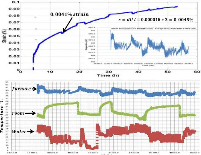
Figure 4.3: Preliminary creep test at 900 °C, at stress level of 1 MPa for 24 hours 51 Figure 4.4: Linear regression line fitting of preliminary creep data 53 Figure 4.5: Change in creep strain due to change in temperature as effect of thermal expansion 54
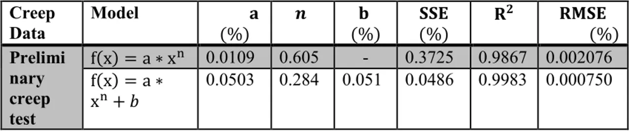
Figure 4.6: Curve fitting of power law models 55
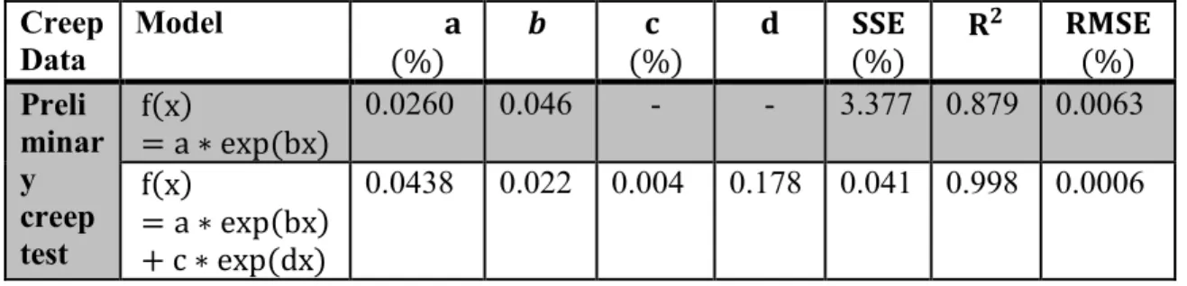
Figure 4.7: Curve fitting of exponential models 56
Figure 4.8: Curve fitting of preliminary creep data with Burger model 57 Figure 4.9: Creep test data at 900 °C, at a stress level of 0.5 MPa 59 Figure 4.10: Creep test data at 900 °C, at a stress level of 1 MPa 59 Figure 4.11: Creep test data at 900 °C, at a stress level of 1.5 MPa 60 Figure 4.12: Comparison of creep test data at three stress levels (0.5, 1, 1.5 MPa) 60 Figure 4.13: Creep test data at 900 °C, at a stress level of 2 MPa 61 Figure 4.14: Comparison of creep test data at all stress levels (0.5, 1, 1.5, 2 MPa) 61 Figure 4.15: Curve fitting of the creep data at a stress level of 2 MPa with Burger model 63 Figure 4.16: Inspection on the circumferential surface of a virgin sample 65 Figure 4.17: Inspection on the circumferential surface of a creep tested sample at 1.5 MPa 65 Figure 4.18: Inspection on the circumferential surface of a creep tested sample at 2 MPa 65 Figure 4.19: Inspection on the top contact surface edge of a virgin sample 66 Figure 4.20: Inspection on the contact surface edge of a creep tested sample °C, at 2 MPa 67 Figure 4.21: Inspection on the contact surface edge of a creep tested sample at 1.5 MPa 67
xiii Figure 4.22: Inspection on the contact surface edge of a creep tested sample at 1 MPa 68 Figure 4.23: Inspection on the contact surface edge of a creep tested sample at 1 MPa 68 Figure 4.24: Inspection on the circumferential edge of a virgin sample 69 Figure 4.25: : Inspection on the circumferential edge of a creep tested sample at 2 MPa 70 Figure 4.26: Inspection on the circumferential edge of a creep tested sample at 1.5 MPa 70 Figure 4.27: Inspection on the circumferential edge of a creep tested sample at 1 MPa 71 Figure 4.28: Inspection on the circumferential edge of a creep tested sample at 1 MPa 71 Figure 4.29: Schematic layout of modified creep test set-up 73 Figure 4.30: Creep test at 900 °C, 0.1 MPa, (a) overall view, (b) zoomed 74 Figure 4.31: Creep test at 900 °C, 0.1 MPa, (a) old setup, (b) modified setup 76 Figure 4.32: Creep test at 900 °C, and a stress level of 1 MPa 77 Figure 4.33: Creep strain rate vs time of test at 900 °C, and at 1 MPa stress level 78 Figure 4.34: Physical inspection on test sample at 900 °C, and a stress level of 1 79 Figure 4.35: Creep test at 900 °C, and a stress level of 2 MPa, 79 Figure 4.36: Creep strain rate vs time of test at 900 °C, and at 2 MPa stress level 80
xv
List of Tables
Table 2.1: Review of various applicable models to represent the creep of metals 28
Table 2.2: List of existing viscoelastic models. 30
Table 3.1: List of equipment for the compression creep test 40 Table 3.2: Measurements of specimen for oxidation and metal loss test (grams) 42 Table 3.3: List of samples for microstructural analysis 45 Table 4.1: Power law models and goodness of fit parameters 55 Table 4.2: Exponential models and goodness of fit parameters 56 Table 4.3: Burger model and goodness of fit parameters 57 Table 4.4: Mechanical parameters of preliminary creep test curve. 58 Table 4.5: Mechanical parameters of Burger model at a stress level of 2 MPa. 63 Table 4.6: Summary of microstructural inspection carried out 64
xvii
Acknowledgement
First and foremost, I would like to thank God for the strength and ability to carry out this study as a partial fulfilment requirement for the Master degree programme in civil engineering from the Université Laval.
I also want to acknowledge the financial support of Natural Sciences and Engineering Research Council of Canada (NSERC) and Alcoa through the Industrial Research Chair MACE3. I would like to also thank the CQRDA and the Aluminium Research Centre-REGAL for partial financial support.
Special thanks to my thesis director, Professor Mario Fafard and co-director Professor Houshang Alamdari for the opportunity to be part of the research group and for their guidance and support throughout this research work.
My appreciation also goes to Dr. Donald Picard, Mr Guillaume Gauvin, Mr Hugues Ferland from the REGAL group, at Laval University for their technical support, and also Mrs Lyne Dupuis for her administrative support. I couldn’t have gotten through without them.
I would also like to extend my appreciation to Dr. Donald Ziegler from Alcoa Canada Primary Metals for the scientific discussions and to Mr André Ferland, and Mrs Maude Larouche from Laval University for their help with the microstructural investigation. Finally, special thanks to my family and my dear wife, Mrs Damilola O. Oyelade for their moral support, encouragements and for standing by me through it all. They made it possible and worth the effort. Thank you to all my colleagues at REGAL group – Laval University and MACE3; it has been an amazing experience and time spent with everyone.
1
1. Introduction
1.1. Basics of aluminium production
Aluminium is the second most produced metal in the world next to iron. It is presently regarded as the third most commonly available element after oxygen and silicon due to the abundant availability of its principal ore, bauxite in the earth crust. Alumina (Al2O3)
is firstly obtained from bauxite by Bayer process, a method well described in literature. After many attempts by previous scientists, in 1886, Charles Martin Hall and Paul Héroult independently and almost simultaneously discovered the process of extracting pure aluminium metal from its alumina by electrolysis process at high temperature of about 970 °C. The overall cell reaction can be expressed as:
2 3 2
2Al O dissolved 3C s 4Al l 3 OC (1.1) This process, now popularly referred to as Hall-Héroult process is well described by several authors [1–3], and is as illustrated in Figure 1.1.
Figure 1.1: Cross sectional schema of an industrial Hall-Héroult electrolytic cell with prebaked anodes. [1]
The basic principle of the Hall-Héroult process has remained unchanged over the last decade. However, its efficiency has increased tremendously and continuously after many refinements and improvements through scientific and technological progress. It is
currently the most widely used method for large scale production of aluminium metal within the industry.
Cost related factors acts as a driving force for the continuous interest from the aluminium industry. Efforts of researchers aim to reduce energy consumption, improve efficiency, maximize productivity and obtain a longer service life of the cell. This has led to new development within the industry, one of which involves an increasing lifespan of the cell from 1000 days in the early years (1948) to close to 2500 days (presently) [2]. Continuous efforts are also dedicated towards full and accurate computerisation of the smelting cell, looking at global and individual components of the cell, their properties, how they function, and the best approach to upgrading their performance in view of optimisation.
Major developments in improving the energy efficiency and the lifespan of the cell were mainly due to the improvements in material quality, operational procedures, innovations in the cell design as well as process automation [2,3]. This approach takes into account, a wide range of complex phenomena such as the behaviour of the anode, the cathode assembly, heat loss, chemical reactions and thermal effects during operation of the cell. This thereby highlighted the need to understand and characterise the behaviour of major and specific components of the cell at operating conditions.
The following sections give a short breakdown of the Hall-Héroult cell, stating the basic motivation for the study on the material behaviour of the cathode collector bar at the cell operating conditions with an eye towards characterisation.
1.2. Breakdown concept of aluminium production
1.2.1. Hall-Héroult cell
The Hall-Héroult cell is governed by Faraday´s law of electrolysis. It is a process where aluminium metal is separated from oxygen by passing an electric current through a melt composed essentially of dissolved alumina in cryolite at temperatures up to around 970 °C (Figure 1.1). Typical cells are operated at low voltages (e.g. 4-5 V) and high electrical currents (e.g. 100 -350 kA) [1,2]. High electrical current enters the reduction cell from the top of the cell through the anode structure, passes through the cryolite bath, through a
3
molten aluminium metal pad, enters the carbon block, and exits the cell through the collector bars.
1.2.2. The cathode assembly
The longevity of the cell at operating conditions is determined by the first material to fail in the cell lining [2]. The entire lower cell construction is usually referred to as the cathode (Figure 1.2a) and is well described in literature [2–4]. In this study, the cathode assembly can be simply described as being made up of three major parts, consisting of the aluminium metal pad, the carbon blocks and the steel collector bars (Figure 1.2b).
Figure 1.2: A typical cathode assembly, (a) the cathode (b) side cut away of multiple cells showing the aluminium pad, (c) two collector bars embedded in the carbon block. [2–4]
The carbon block are preformed rectangular blocks made up of carbon composite and occupies the full width between in sidewalls of the cell. In a conventional cathode today, the base of each carbon block is embedded with one or two steel rail bars (collector bar) that extend to the open ends of the steel shell and through each side of the electrolytic cell to connect with the bus bar (Figure 1.2c).
(b)
1.2.3. The steel collector bar
The collector bar serves as an electrical current collector and runs horizontally through the entire bottom lining. It is made of low carbon steel with carbon content of about 0.08 %C to obtain and maximise good conductivity and ductility properties of the bar. Steel however, has high thermal conductivity and deforms at high temperatures. The steel cathode collector bars are attached to the carbon blocks using cast iron poured during sealing operations (see Figure 1.3c), carbon glue, or rammed carbonaceous paste. The method of pouring cast iron to seal the collector bar to the carbon block is preferred and more popular as it facilitates good contact and reduces the electrical resistance at this interface, thereby reducing the overall voltage drop in the cathode assembly.
1.3. Problem
1.3.1. Introduction
There is a continuous fundamental need of the aluminium industry to better understand the degradation mechanism of the electrolysis cell lining in order to further improve its conception. The average life of the aluminium reduction cell is presently at about 2500 days for most smelters. This is less than the maximum life (about 3000 – 4000 days) that could be achieved if limitations were only due to the erosion of the carbon blocks [2,3]. However, many other mechanisms also contribute to the pre-mature failure of the cell lining, and in order to maximise the service life of the cell, a better knowledge of these mechanisms is required.
1.3.2. Failure mechanism in the cathode assembly
During operation, the cathode blocks are subjected to the action of high temperature and chemical process, which promote the degradation, heaving of the carbon blocks and cracking the cathodes. Many phenomena contribute to the heaving of the carbon blocks including stresses induced by thermal expansion, sodium swelling and chemical reaction inside the carbon blocks and side materials. However, these mechanisms and their effects have been well studied in literature [2,5].
5
1.3.3. Deformation of the steel collector bar
At high temperature, the cathode collector bar undergoes thermal expansion and exhibits greater expansion than in the carbon block (Figure 1.3a). During the sealing operation of attaching the collector bar to the carbon block, the expansion of the bar is not monotonic in behaviour. In the vicinity of 750 - 900 °C, the collector bar contracts, leading to the gap evolution (Figure 1.3b). The contact resistance between the collector bar and the cathode block has been previously estimated at 10 Ωmm2 contributing roughly 100mV to the cell voltage drop in the cathode assembly [4].
Figure 1.3: Effect of thermal expansion on the cathode assembly. (a): deformation curve for the carbon block and the steel collector bar; (b): deformation and gap evolution, (c)
assembly of the carbon block, cast iron and steel bar. [4].
The voltage drop over the cathode assembly due to increase in electrical contact resistance of its components is an important indicator of the cathode´s condition. As the cell gets older, the cathode voltage drop increases in a more or less regular manner [4]. This increase in contact resistance of the cathode assembly is also a consideration in the design of the pot-to-pot electrical busbar as it impacts the current distribution.
Autopsies also showed that the heaving of the cathode carbon block induces a considerable deformation profile in the collector bar (Figure 1.4), majorly due to the temperature gradient and lower constraints at the end of the bar [2]. This leads not only to
(b)
elastic contractions but also creep of the cathode collector bar over the service life of the cell [5]. The total strain can be expressed such that:
(1.2)
denotes total strain, thermal strain, elastic strain and creep strain [2,5,6].
The creep/relaxation behaviour is a nearly incompressible phenomenon. The deformation along the transverse section of the collector bar causes a decrease in the stress level at the steel/cast iron/cathode block interfaces, thereby further increasing the electrical resistance induced at this interface. This also contributes to the overall contact voltage drop (CVD) in the cathode assembly hence reducing the energy efficiency of the cell.
Figure 1.4: Deformation of the collector bar: (a) deformed collector bar, (b) measurement of deformed collector bar after service life. [2]
Steel has excellent strength properties at ambient conditions, but loses its strength and stiffness with increasing temperature. At high temperature, deformation becomes more pronounced even at low stress level as the yield strength becomes significantly lower. A more dominating creep effect also begins to occur with time at high temperature.
In order to have a good understanding of the material behaviour of the collector bar at operating temperature (around 960 °C), it is necessary to identify parameters not only for thermal expansion and elastic behaviour, but also for the creep behaviour of the metal.
(b) (a)
Inside the cell Outside the cell
7
1.4. Deformation behaviour and properties of metals
1.4.1. Thermal properties
Metals, as all materials, deform in response to a change in temperature. This deformation behaviour is termed as thermal expansion. The level of deformation by the change in temperature is commonly used to determine the material´s coefficient of thermal expansion. This data are well stated in the literature [7,8] for different materials and at different temperatures. It can be obtained by expressions such as:
(1.3)
where denotes thermal expansion coefficient, initial length, change in length due to change in temperature .
1.4.2. Mechanical properties - stress – strain – time relationships
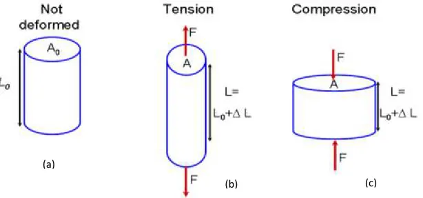
Metals subjected to a uniaxial force will undergo deformation which may be time-dependent or not. The properties of metals and their alloys are highly influenced by their microstructure. Their deformation behaviour is dependent on the applied stress and temperature which influence the microstructure of the metal. Deformation of metals through application of mechanical loads in tension or in compression is as illustrated in Figure 1.5.
Figure 1.5: Sketch of a material under various modes of applied load: (a) no load, (b) in tension, and (c) in compression
A simply applied load � is distributed on the surface area of a specimen resulting in distributed stress , which can be expressed such as:
F A
(1.4)
This results in deformation of such material where the new length is calculated such as:
(1.5)
where is the original length (also referred as gage length) before deformation, is the change in length and is the final length upon deformation. The strain can be obtained by:
0
L L
(1.6)
In a general form, the strain increases with increasing level of stress. The stress-strain data plots are typical for explaining the deformation characteristic of many materials and for obtaining their mechanical properties [9]. This process is well described in literature and as illustrated in Figure 1.6.
(a)
9
Figure 1.6: Stress – Strain curve, typical for a material in tension: (a) material behaviour and parameters along the curve, (b) types and regions of occurring deformation. [8,9]. Strain regions of elastic, plastic, necking and fracture can be observed in Figure 1.6b. This is characteristic for a ductile metal in elongation, but slightly different in compression as necking is not observed in such case. The essential region of the curve can be briefly explained as follows:
Elastic deformation is a reversible process where material regains its original dimension on removal of applied load. The deformation behaviour governed by the Hooke´s law such that:
/
e E
(1.7)
where is the applied stress in the elastic domain, the modulus of elasticity (Young´s modulus) and is the elastic strain. Apart from elastic deformation that disappears on removal of stress, even more deformation behaviour can occur with increasing stress range above the yield strength of such material. These types of deformation are usually referred to as “inelastic deformation” and can be either “plastic deformation” (occurring at stresses beyond yield stress and time independent) or “creep deformation” (occurring on application of constant stress over a time period) or action of both.
Plastic deformation is a permanent strain occurring at region above the yield strength of the material. At onset of plastic deformation, a small increase in stress causes a relatively large additional deformation independent of time. This process of further
deformation is called yielding (occurring strain hardening), where the peak value is the ultimate strength of the material before tending towards fracture.
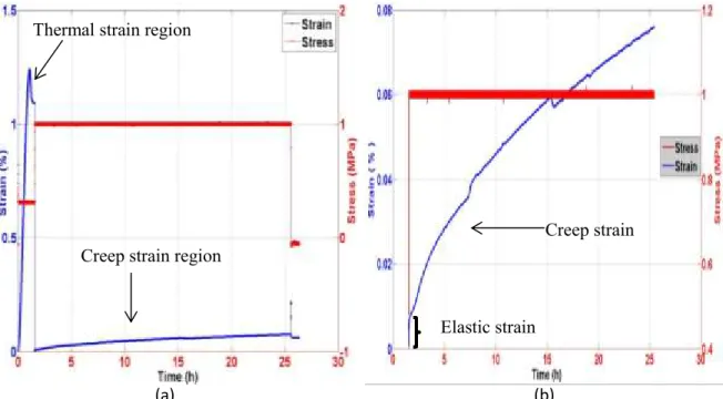
In addition to time independent elastic and plastic deformation described earlier, materials also undergo inelastic deformation at constant stress by mechanisms that result in markedly time-dependent behaviour called creep. This behaviour is represented by a curve where the strain varies with time (Figure 1.7). In this curve, there is a region of instant elastic deformation , (instantly recoverable on removal of stress), primary creep strain (mainly recoverable with time), secondary creep strain (steady state and permanent strain), and the tertiary creep strain tending towards rupture.
Figure 1.7: Schematics of a typical uniaxial creep curve. [9]
Fracture and rupture as described in Figure 1.6 and 1.7 respectively are terms related to damage which is not experienced by the cathode collector bar in the cell. Therefore it has not been considered in this work.
1.5. Scope of work - objectives
To sustain the continuous increase in the cell´s service life, the characterization of the material behaviour of the collector bar is a major factor that must be taken into consideration, especially for developing an accurate numerical model of the cell.
11
Therefore, the study of the deformation behaviour of the collector bar at conditions experienced within the aluminium reduction cell is of great importance to further optimize the energy efficiency and increase the life span of the cell.
There is a lack of sufficient relevant data in the literature to fully characterize the deformation behaviour of the collector bar at operating condition. Hence, in this study, an experimental procedure was carried out on the steel collector bar material (AISI 1006) to investigate its deformation behaviour in relation to its thermal, elastic and creep properties. The tests were carried out in compression at high temperature and low stress levels to reproduce conditions experienced within the reduction cell. The following objectives and considerations were set out in order to achieve this:
state of art literature review of previous researches on the material properties of the metals at high temperature, phenomenon of creep in metals, time-dependent deformation theories and rheological models of creep theories;
experimental investigations, by carrying out compressive creep tests at constant temperature of 900 °C and at different constant stress levels of 0.5, 1, 1.5 and 2 MPa;
considerations for the effect of thermal expansion and phase change; considerations for the effect of corrosion and oxides;
microstructural inspections on both virgin and tested samples; fit of suitable models and obtaining material parameters.
1.6. Structure of thesis content
The second chapter covers a state of art literature review looking at previous researching and discussing findings of existing data in relation to material properties of metal at high temperature, the creep phenomenon, creep theories and rheological models used in representing deformation behaviours of metals.
Chapter three looks at the experimental program from material selection, preparations including test set up and procedures, limitations and considerations for environmental factors having effect on deformation behaviour. Chapter four shows the results obtained
including those of corrosion tests, thermal expansion at heating period, creep tests and metallography inspections. It also looks at the analysis of obtained experimental results, discussing observations in the deformation behaviour at different stress levels up to 2 MPa and the outcome of the microstructural investigation carried out on virgin and tested samples.
The last chapter, chapter six, summarises all observations from methodology, obtained results and analysis approach, drawing conclusions based on chapter four. Theories discussed to try to explain observed behaviour and recommendations for future research were also looked at.
13
2. Literature Review 2.1. Background
Metals generally deform when subjected to high temperature and applied stress conditions. Hence, cathode collector bar, subjected to developed stresses at elevated temperature of up to 960 °C, undergoes not only elastic deformation but also creep of the bar over the service life of the cell. Good understanding of the time-dependent stress – strain relationship are therefore required to study, understand and model the behaviour of the bar at such high temperature conditions of the cell.
A literature review on the material properties of metals at high temperatures, physical mechanism of creep, characteristic creep behaviour at elevated temperature and low stress levels, and general model representations of such behaviour was deemed necessary. In line with the objectives of this work, this was carried out and summarised in this chapter.
2.2. Material Properties at High Temperature
2.2.1. Introduction
Although steel has excellent strength properties at ambient conditions, it loses its strength and stiffness with increasing temperature. At high temperature, deformation becomes more pronounced even at very low stress level, as its properties changes significantly. The response of steel structure exposed to high temperature is governed by its thermal and mechanical properties. These temperature-dependent parameters, consisting mainly of thermal strain coefficient, Young’s modulus, Poisson´s ratio and creep data, are required to model the deformation behaviour of the cathode collector bar in the cell. These properties are, however, also majorly affected by the microstructure and composition of the material and should firstly be considered.
2.2.2. Effect of carbon content on material properties
The weakening influence of carbon in carbon steel has been suggested by previous studies [10–12]. The amount of carbon in a metal has a reasonable effect on its thermal, mechanical and creep deformation properties. The carbon content of a steel bar has a
major influence on the temperature range at which phase change occurs during thermal expansion. However, it also has a major effect on the mechanical and deformation properties of the metal. This will be further discussed later on.
Weinberg [10] measured a decrease in the ultimate tensile strength (UTS) of steel with carbon content up to about 1.0 %C while Wray [11], also carried out series of experiments in tension to describe the effect of carbon content on the plastic deformation behaviour of plain carbon steel at elevated temperature up to (1300 °C).
Pines and Sirenko [12] observed that the creep strength of austenite steel decreased continually with increasing carbon up to about 1.0 %C. Ruano et al[13] also related the change in creep strength of steel to the measured increase in the self-diffusivity of iron with carbon. Ruano further suggested that an increase in self-diffusivity is an indicative of weaker interatomic bonding as results showed that the austenitic iron lattice is expanded by the addition/increase in carbon.
2.2.3. Thermal properties
Major parameters influencing the temperature rise in steel are thermal conductivity and specific heat (or heat capacity). The thermal conductivity decreases with increasing temperature in an almost linear fashion (Figure 2.1a) while the specific heat increases with increasing temperature and have a large spike occurring at 750 °C (Figure 2.1b).
15
Figure 2.1: Effect of increasing temperature on low carbon steel thermal properties (a) thermal conductivity, (b) specific heat. [8]
The spike in the specific heat at about 750 °C is due to phase change occurring in the steel microstructure, the point at which transition of atomic structure from a face centred cubic (FCC) to a body centred cubic (BCC) begins to occur. This also corresponds with the deformation behaviour of steel where carbon steel undergoes linear thermal expansion with increasing temperature (Figure 2.2a).
Figure 2.2: Effect of temperature on steel deformation properties: (a) variation of thermal strain with temperature, (b) iron – carbon phase diagram. [7]
(a)
(a)
(b)
At a certain temperature, the linear expansion changes and material begins to contract over a short range of temperature before any further increase. This contraction region is a result of the occurring phase transformation, where material moves from ferrite to austenite temperature region. Due to high dependence of the material properties on the microstructure (e.g. material composition), the carbon content of the steel bar has a major influence on the point at which the phase transformation begins (Figure 2.2b).
At carbon content above 0.02 %, a phase change from ferrite to austenite associated to a contraction, starts to occur at about 730 °C and finishes between 800 °C and 900 °C for carbon content up to 0.3 %. A thermal strain of up to 1.2 % with the occurrence of a phase change has been predicted by different models and measured in different tests at temperatures up to 900 °C [7,8].
2.2.4. Mechanical properties
The mechanical properties of metals are generally represented within the stress–strain diagram (see Figure 1.6). Strength tests are usually conducted either in transient (constant load, increasing temperature rate) or at steady state (constant temperature, increasing load rate) to obtain the stress-strain plot where the mechanical properties such as Young´s modulus, yield strength, strain hardening parameter, ultimate strength and even fracture parameters can be estimated.
Tensile strength test is the most popular method used [8,9,14,15] to obtain the mechanical properties for most metals and their alloys. There is limited data found in literature for tests in compression. However, it is generally assumed that the Young´s modulus, derived based on tensile strength tests are the same for compression state. For low carbon steel in tension, both yield strength and elastic modulus decreases significantly at higher temperatures above 300 °C. Existing data at different temperatures shows an elastic modulus of about 13.5 GPa and a yield strength of 18 MPa (at a loading rate of 0.01 s-1) have been measured in different tests at 900 °C (Figure 2.3) [8].
17
Figure 2.3: Normalised data of mechanical properties at different temperatures: (a) yield strength vs. temperature, (b) Elasticity modulus vs. temperature. [8]
Compression test data on the collector bar material (AISI 1006) showed great influence and dependence of its deformation behaviour and mechanical properties on temperature up to 850 °C for strain rates ranging from 0.1 to 50 s-1. At constant temperature of 850 °C, the yield stress increases with increasing strain rate such that, yield stresses of 50, 85 and 150 MPa were obtained for strain rates of 0.1, 3, and 50 s-1 respectively [16].
European standard, EC-3 distinguished the proportionality limit of a material as the end of the linear elastic portion of the stress – strain curve (Figure 1.6), point after which it becomes nonlinear elastic before the yield limit is reached. This approach was deemed necessary to partly account for creep strain in test sample subjected to strength test at high temperatures [15].
2.2.5. Creep properties
Deformation properties influencing response of steel structures at elevated temperatures are thermal strain and creep at high temperatures. A brief introduction to the creep deformation behaviour of materials was carried out in chapter one (see Figure 1.7). A study on the creep rate of the collector bar at low loads ranging from 1 to 5 MPa [7] concluded that the collector bar slowly deformed under small forces experienced in the cell at temperatures above 700 °C. From several data provided in this study (Figure 2.4),
it can be concluded that the creep rate is around 0.002 %/h at 900 °C under a load of 1.3 MPa, a rate corresponding to almost 1 % creep in three weeks [7].
Figure 2.4: Creep rate data at different stresses & temperatures. [7]
To fully understand the creep deformation behaviour and properties of a material, it is necessary to study the creep phenomenon including the mechanism, physical laws and models used to represent and explain such behaviour.
2.3. The phenomenon of creep
Creep is a time-dependent deformation where under constant stress, the strain varies with time (
). Creep of solid may be exhibited in the visco-elastic range where the
creep strain may be completely (or almost completely) recovered on removal of the stress, or in visco-plastic range, where the creep deformation is permanent. In the latter case (permanent deformation), an elastic component also exists but this may be trivial by comparison [9].
A typical creep curve can be characterised by three stages; primary, secondary and tertiary (see Figure 1.7). In the initial stage “primary creep”, the strain is relatively high
19
but slows down with increasing time (decreasing strain rate) and eventually reaches a steady state named “secondary creep” (constant strain rate). In the final stage “tertiary creep”, the creep strain accelerates (increase in strain rate) towards failure. This final stage is mostly observed in a tensile test rather than compression due to the “Necking” effect.
Creep strains are derived from steady state tests during which the stress is kept constant. The extent of creep deformation in a given material is dependent on and can be characterised by the applied stress level and temperature level at which the test is being carried out. An increasing level of creep strain can be obtained in response to an increased level of the applied stress and/or temperature (Figure 2.5).
Figure 2.5: Schematic view of a typical creep curves for various stresses and temperature levels. (a): increasing stress level, (b) increasing temperature level. [8]
There is a stress level ( in Figure 2.5a), popularly referred to as “threshold stress”, and a temperature level ( in Figure 2.5b), where the resulting creep strain is very small or negligible. Below these levels, no creep strain is considered to occur [17]. Increasing temperature above threshold ( in Figure 2.5b) leads to a stress driven atomic rearrangement in the microstructure of the material hence acting creep deformation over time. Such case is referred to as thermally activated creep process, which takes into account, the dependence of both stress and temperature and is governed by the Arrhenius equation:
̇ ( ) (2.1)
depends mainly on the material, is the activation energy which can be altered due to a sufficient shift in temperature or stress, is the applied stress, ̇ is the strain rate and is the temperature [18,19].
The secondary creep stage is considered as the most understood of the creep stages and deemed important for explaining the creep deformation behaviour of metals [18]. The stress dependence parameter n, of the creep curve for this stage depends on the creep rate and the applied stress. This has been well explained by different creep mechanisms in literature. A creep rate - time curve (Figure 2.6) is generally used to give a clearer identification and understanding of the creep curve and to determine the dominating creep mechanism.
Figure 2.6: Schematic view of a typical uniaxial creep rate curve. [18]
Similar and derived from the creep curve, the creep rate versus time curve has a primary creep stage, where the creep rate decreases with time ( ). A clear section of the secondary creep stage is observed where the strain rate reaches a near constant (
21
) and also referred to as “minimum strain rate”. In the final stage, tertiary creep, the strain rate accelerates towards rupture ( ).
A general equation for the secondary creep rate in crystalline material is often derived from Arrhenius equation above such that:
̇ (2.2)
where is the average grain diameter, absolute temperature, the stress coefficient, the grain size coefficient and is the activation energy [19].
Generally for metals under constant load, creep is expected to become noticeable at temperatures corresponding to 30 % of the melting temperature (0.3Tm) for pure metals
and 40 % (0.4Tm) for alloy metals [19]. For the cathode collector bar material sample
(AISI 1006) used in this study, the melting point is at approximately 1400 °C. Therefore the creep strain should become evident at temperature starting from 566 °C and above. Earlier published works focused on creep behaviour of metals and observed that the physical mechanism causing deformation is quite different from that in other solids. In crystalline materials such as metals, the creep curve is related to possible action of a group of mechanisms which depends not only on certain temperature and stress ranges but also depends on the structure of the alloy, its composition and the pre-history of the sample/material [13,20,21].
Therefore it is important to further investigate and understand the mechanism causing creep in crystalline material particularly in steel metals. This is considered and summarised in the next section.
2.4. Physical mechanisms of creep:
2.4.1. Microstructural behaviour
Polycrystalline metal aggregates consist of crystal grains with characteristic arrangement of atoms within them. The basic mechanism of deformations of these grains is that its part slips relative to each other. This slip occurs in places close to the packing of atoms and may be understood by taking into account the motion of crystal defects, known as dislocations [9].
Dislocation slip and grain boundary sliding are important mechanisms that determine material´s mechanical behaviour. Dislocations are linear defects in the crystal structure of metals and are largely responsible for the material´s inelastic deformation. Elaborate interactions between the defects in a crystal structure can lead to complex forms of mechanical behaviour.
For example, in response to a stress applied on a material, the crystal structure consisting of atoms, vacancies, dislocations within the solid material moves relative to one another in a time-dependent manner, resulting in creep deformation (Figure 2.7). Such atomic motion occurs more rapidly at higher temperature and constitutes a broad category of behaviour process called diffusion.
Figure 2.7: Defects in a metallic crystalline structure, (a) line dislocation, (b) dislocation screw, (c) point defects. [9]
(c)
23
At low temperature (below 0.3Tm), creep deformation occurs at a very slow time pace as
the amount and distribution of the defects in the crystal structure remains almost uniform (dislocation slip/slide mechanism). However, at high temperature, creep deformation occurs at a faster rate as vacancies in the crystal structure diffuse to the location of dislocations and causes them to accelerate to adjacent slip plane.
Variety of physical mechanisms, explaining creep process in metal and its dependence on the applied stress and temperature, have been widely studied in literature [18]. They may however, be grouped into two terms as “diffusional flow” and “dislocation flow”. Considerations are sometimes given for grain boundary sliding (GBS) to be a distinct mechanism.
2.4.2. Dislocation slip mechanism
This creep mechanism is a kinetic process occurring at low temperatures between 0.1Tm and 0.3Tm. Below the ideal shear strength, flow of dislocations by glide motion can occur, provided a sufficient number of independent slip systems are available (Figure 2.8). This will cause the material to undergo work hardening until the stress required to flow equals the applied stress. However, this motion can be limited by obstacles such as solutes, precipitates or even grain boundaries [18].
Figure 2.8; Mechanism of dislocation slip. (a) motion obstructed by obstacles (b) slip of weak grain boundary. [18]
2.4.3. Diffusional creep
This creep mechanism occurs at low stresses and relatively high temperature (above 0.6Tm). It involves the movement of vacancies in the crystal lattice (Figure 2.9). This can occur as a result of spontaneous formation of vacancies near the grain boundaries that are approximately normal to the applied stress. The uneven distribution thus created results in movement (diffusion) of the vacancies to regions of lower concentration. This leads to a mass transfer in the material structure, causing an overall deformation of the material.
Figure 2.9: Mechanism of diffusion creep, (a) lattice and boundary diffusion of vacancies and atoms respectively (b) response of defects to an applied stress. [18]
Physical laws of diffusional flow mechanism are explained either by (a) lattice diffusion (Nebarro – Herring creep), or (b) grain boundary diffusion (Coble creep). Nebarro Herring creep occurs if the vacancies move through the crystal lattice while Coble creep occurs if the vacancies move along grain boundaries instead and represented by:
̇ ( ) ( )
( ) ̇ ( ) ( )
( ) (2.3) where they both have a strain rate ̇ approximately proportional to the stress , a stress exponent (n) of 1 (i.e. linear behaviour), an inverse proportionality to the square of the average grain diameter (for Nebarro, grain dependence q = 2 and for Coble, q = 3), the shear modulus and the Burger´s vector constant [18,19].
25
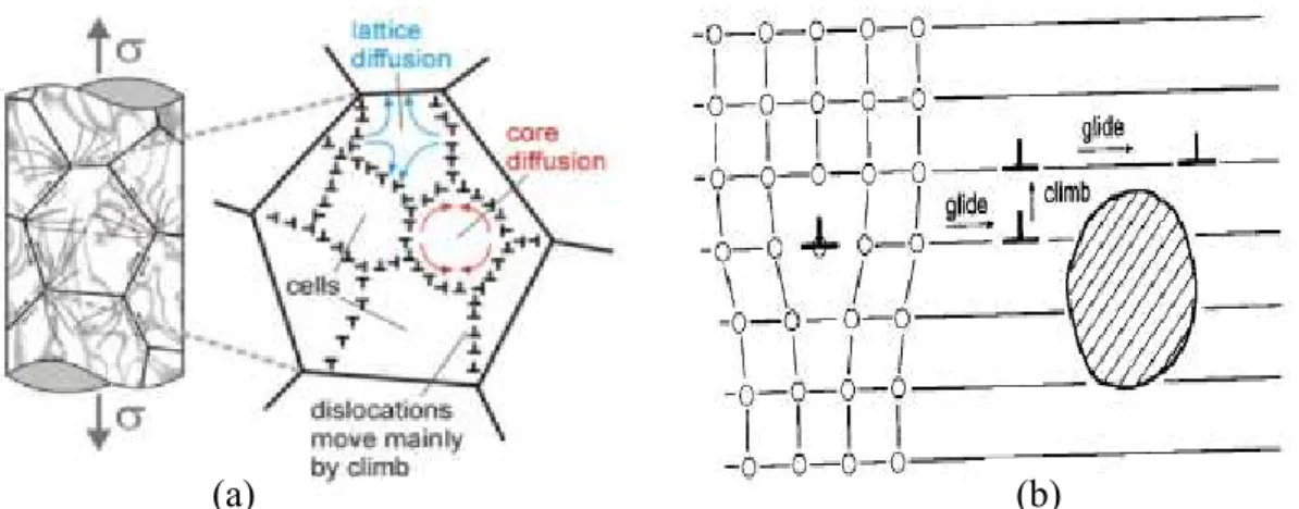
2.4.4. Power law creep - dislocation climb
This creep mechanism occurs at intermediate temperatures (0.3Tm - 0.6Tm) and relatively
high stress level. This process employs the flow of dislocations by both glide motion and climb over obstacles through movement of vacancies (Figure 2.10). In response to an applied stress on a material, an edge dislocation moves along the crystal plane by stepwise slip process (glide). On encountering an obstacle, such as a precipitate particle or an immobile entanglement of other dislocations, further deformation requires that the dislocation move to another lattice plane. This motion is termed “climb” and requires rearrangement of atoms by vacancy diffusion. The climb process is time-dependent and considered to have a more dominating effect in the creep deformation behaviour of the material. The cumulative effect of a large number of such climb events permits more slip (glide), hence permitting more macroscopic deformation to occur [18,19].
Figure 2.10: Climb plus glide controlled creep mechanism in power law (a) effect of lattice diffusion + dislocation climb (controlling effect), (b) Dislocation climb + glide
effect. [18].
The resistance to the climb process is such that considerable high stress is required for deformation to occur. Hence, the power law creep theory has a strong stress dependence factor , with values ranging from three to eight. The representative equation can be expressed such that [19]:
̇ (
) ( ) (2.4)
2.4.5. Harper - Dorn creep
Creep experiments are difficult to carry out at low stresses. This is because strain rates are very low and a very high level of precision is required. This made it very difficult to predict and develop an accurate physical mechanism at such conditions. However, Harper and Dorn in a study in 1957 proposed a physical mechanism to predict creep of metals at low stress level and high temperature (above 0.6Tm). Numerous creep tests were
performed on aluminium of high purity and large grain sizes [19,22]. Results of the investigation lead to the conclusions that (a) the steady state creep rate increased linearly with the applied stress (i.e. stress exponent n =1), (b) no dependence on grain size, (c) similar to power law, dislocation-climb is the controlling mechanism and the activation energy was that of self-diffusion (Figure 2.11).
Figure 2.11: Creep strain rate – stress plot (a) physical laws occurring at different stress and strain rate region, (b) Evidence of Harper Dorn and Nebarro creep laws. [19].
The relationship between the applied stress and the steady state creep rate for the Harper-Dorn creep can be phenomenologically described similar to power law as:
27
̇ (
) ( )
(2.5)
is Harper Dorn constant and a stress exponent of [19].
Similar observations were also reported some years later by other investigators, although the effect of dynamic recrystallization was also observed for tests at high temperatures above 0.6Tm [22,23].
2.5. Representation of creep behaviour models
2.5.1. Background
The fundamental problem of modelling creep behaviour is the representation of the stress – strain – time relationship. This is a complex phenomenon and has large number of factors influencing it. Several models and theories other than those identified in the previous section have been developed to describe creep behaviour in a wide range of real materials; they will be looked at further on in this study.
The record of creep behaviour and regions within the creep curve has been discussed earlier in this chapter. Some of the physical mechanisms and laws developed to understand them were also considered. Various models to represent these creep behaviour have been widely studied in the literature [24–30]. A few of such relevant models for metals were reviewed here with respect to applicable creep regions and their ability to represent the dependence of stress, temperature and internal variables parameters of the creep curve are summarised here.
2.5.2. Phenomenological models
Phenomenological models are theories of creep, developed based on the observation of experimental creep curves, obtained by testing a number of identical specimens under creep / relaxation condition. The models are based on the study of the stress – strain – time deformation behaviour of metals in the laboratory at required conditions (different stress and temperature levels). It purely tries to characterise the stress – strain and or the
strain - time curves obtained from experimental data by using known phenomena and obtaining its parameters by curve fitting and regression.
Stress - strain rate curve parameter plays a significant role in modelling the creep behaviour. Steel may be considered as an isotropic incompressible material, where similar to plasticity theory, the creep behaviour may be divided into volumetric and deviatoric (or shear) parts. Only the applied deviatoric (shear) stress, causing deformation of the material (deviatoric strain), will be considered in this study.
Models based on phenomenological behaviour of metals uses physical quantities or try to introduce meaning to the used parameters and its applications are only possible for given conditions. Different phenomenological models for stress-strain behaviour have been proposed by many authors [24–30]. These models are further looked at in the next section.
2.5.3. Empirical models
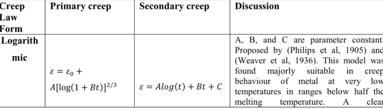
Empirical creep models were generally derived using observed data from relationship between stress – strain – time in the creep test. The parameters involved, e.g. the stress exponent n, can be determined by curve fitting of the test data. Each region of the creep curve, (primary, secondary and tertiary) can be described by its own special equation. Different groups of fundamental equations were developed along the line of logarithmic form, sine-hyperbolic form, polynomial form and exponential form. Each form was reviewed to describe models for both primary and secondary creep. This is summarised in Table 2.1.
Table 2.1: Review of various applicable models developed to represent the creep of metals
Creep Law Form
Primary creep Secondary creep Discussion Logarith
mic
A, B, and C are parameter constant. Proposed by (Philips et al, 1905) and (Weaver et al, 1936). This model was found majorly suitable in creep behaviour of metal at very low temperatures in ranges below half the
29 disadvantage of the model is that stress and temperature dependencies of the parameters are not explicitly accounted for. Sine -hyperboli c [ ( ) ] ( ) ( ( ))
Proposed by (Parker et al, 1958) and developed for secondary creep by Nadai – McVetty in 1943. Due to the nature of this relation (hyperbolic function), it defines a linear relation between creep rate and stress at low stress values. To describe the temperature dependencies, additional Arrhenius term should be multiplied to this relation.
Polynomi al
n and p are parameter constant. Model developed by (Norton, 1929) and (Bailey, 1935), (Andrade, 1914) and (Cottrell-Ayetkin, 1947). The advantage of this model is its power law relation used to describe the stress variable dependent to the elevated temperature. Major disadvantage is the lack of its explicit consideration of the temperature and the fixed exponent of 1/3, limiting its acceptability. Exponent ial ( )
R is a gas constant, Qa is the activation
energy and T is the absolute temperature. Proposed by Sherby, Dorn, 1953. The disadvantage of the primary creep model is that temperature and stress dependencies are not explicitly modelled. It has however served as a pioneer to the development of the Garofalo creep model for the whole creep curve (i.e. secondary and even tertiary stage).The model for secondary creep describes the effect of certain test parameters such as temperature and stress on creep behaviour. It contains nearly all parameter dependencies used in a creep experiment.
In summary of Table 2.1, the mathematical form of all creep relations described above were categorised in forms of exponential, power law, or sine – hyperbolic relations. The explicit forms of this law, which are a function of time, are not applicable for finite element analysis. However, Taylor expansion helps to reduce all creep models to either power law or exponential form.
More developments were seen in modelling of creep behaviour especially in research results reported between 2000 and 2012. Researches focused more on modification and
extension of previous developed models discussed in Table 2.1. A major attempt to describe the creep process was further concentrated more or less on using the exponential approach based on the idea of the Kelvin – Voigt viscoelastic model which are well described in literature [31–33].
2.5.4. Viscoelastic models
The creep behaviour of metals can be represented by models comprising of springs and dashpots to represent elastic and viscous strain respectively. Viscoelastic models proposed by Kelvin - Voigt in 1898 are simple rheological models developed on the idea of the exponential creep law form (Table 2.2). The goal of rheological models is to relate, by laboratory testing, each component of stress to each component of strain while, in the process, introducing a few material properties as is necessary to capture the fundamental behaviour with sufficient accuracy for engineering purposes. Various combinations of these mechanical models such as spring and dashpots can be used (Table 2.2) to simulate a wide range of time-dependent behaviour. Different viscoelastic models are popularly used and well described in literature [30–35]; some of which are also listed in Table 2.2. Table 2.2: List of existing viscoelastic models.
Model Property Stress – strain – time relation in 1D Element representation Spring Elastic Dashpot Viscous Maxwell Viscoelastic
31 Kelvin - Voigt Viscoelastic [ ] Generalized Kelvin Viscoelastic [ ] Generalized Maxwell Viscoelastic [ ] Burger Viscoelastic [ ]
where stress, strain, Young´s modulus, shear modulus, shear strain viscosity, and time.
Different rheological models have been introduced for the mathematical description of the stress-train-time behaviour of metals. However, the basic creep behaviour of metals at high temperature can best be described according to Maxwell, Kelvin-Voigt, Burger (Table 2.2) and the introduction of Bingham (elastoviscoplastic) models.
Maxwell model, proposed by James Maxwell in 1868, combines the elastic element (spring) to the viscous element (dashpot) in series. On application of stress, the elastic element produces instantaneous strain. As the stress remains constant over a certain period of time, viscous flow will occur; this is also referred to as delayed strain. Thus the elastic deformation completely disappears in favour of the viscous component, thereby inducing permanent strain.
Kelvin - Voigt model combines elastic element (spring) to viscous element (dashpot) in parallel. The set-up of this model means elastic and viscous elements can only be deformed together and to the same extent. Hence, unlike Maxwell, instantaneous
deformation on application of stress is not represented. Under a constant load, at the beginning, the dashpot sustains the load alone and gradually transfers the load to the spring.
Both Maxwell and Kelvin - Voigt model are linear viscoelastic models capable of giving a good representation of the regions within a creep curve as described earlier. The elements of Kelvin-Voigt gives a good representation of the primary creep strain region (recoverable strain), while the elastic and viscous element of Maxwell gives a good representation of the elastic strain region and the secondary creep strain region (irreversible viscous flow) respectively. However, for a Kelvin-Voigt element of an established rheological model subjected to an applied stress, the viscous element could also experience a continuous viscous flow; meaning the primary creep strain region may not be fully reversible.
Plastic strain (permanent deformation) behaviour occurs in metals when the applied stress is greater than the yield stress and requires incorporation of an additional element (plastic slider) other than the elastic and viscous element used in Kelvin Voigt and Maxwell models. However, at high temperatures, metals lose their yield strength and can undergo a continuous viscous flow (permanent strain deformation) even at low stresses below its yield stress. In such cases, the use of the elements of Kelvin-Voigt and Maxwell or their combination is still applicable without the additional plastic element.
Linear viscoelastic models have been extended to account for non-linear viscosity representing the effect of permanent strain in the deformation behaviour of metals. One of such approaches included slightly modifying and adding an additional term (n) to the Kelvin –Voigt model representing the primary creep strain region such that:
(2.6)
Garofalo [30] also described the instantaneous elastic, primary and secondary regions of the creep curve by adding linear terms (elasto -plastic part) to the Kelvin-Voigt model such that:
33
where is the initial time independent elastic strain, is the transient (primary) creep strain, is the transient time between primary and secondary creep part and ̇ is the strain rate of the secondary creep region.
Similar to Garofalo model, Burger rheological model combined the elements of Maxwell and Kelvin-Voigt model in series to account for the instantaneous elastic strain, recoverable strain (primary creep) and the permanent strain (secondary creep) region of the creep curve (Figure 2.12).
Figure 2.12: Burger viscoelastic creep model
The equation of the Burger model can simple be expressed in terms of stress and strain such that:
𝜺 𝒕 𝝈 [ { 𝒙𝒑 ( 𝒕 )} 𝒕
𝒑] (2.8)
where is the total strain, is the constant applied stress, is the elastic modulus for the instantaneous elastic region, is the modulus for the viscous recoverable region, is the viscous coefficient of the recoverable region, and is the viscous coefficient of the permanent strain region.
The differential stress – strain constitutive relation of the model can hence be expressed such as:
( )
̇
̈
̇
̈
(2.9) Equation (2.9) is a second order derivative and the determination of the creep integral core function is of importance. At the initial stage, the elastic region, where the stress is a constant at time the creep equation can simply be expressed in its integral core function:∫ (2.10) where is the elastic compliance, is the creep core function and the eigen function which reflects the rheological properties of the material can hence be expressed as:
̇ (2.11) The Burger model can be considered suitable to adequately represent all regions of the creep curve, (including permanent strain due to viscous flow) for metals in deformation at high temperatures and at low stress levels below their yield strength. Maxwell models could also be sufficient to model the creep deformation behaviour of metals in cases where the primary creep strain is negligible. In situations where the applied stress is greater than the yield strength at a particular temperature, the occurring permanent strain (plastic deformation) requires a different model along the line of viscoplasticity.
2.5.5. Elastoviscoplastic models
The Bingham viscoplastic model consists of the Saint Venant rigid plastic element connected in parallel with a Newton viscous element. This model introduces the yield point which describes the transition from the state of rest flow.
The Bingham model equation is such that:
35
where is the applied stress, is the yield stress, is the viscous coefficient and is plastic strain.
Elastoviscoplastic models have been used to model stress – strain - time behaviour in cases where the applied stress exceeds the yield stress of on the material [32]. This model is a slightly modified version of the Burger model and consists of typical kelvin model in series with a Bingham model (Figure 2.13) [31–34].
Figure 2.13: Elastoviscoplastic creep model
The time-dependent stress - strain relationship of the elastoviscoplastic model in 1D is as follows:
[ ] (2.13)
2.6. Summary
This review focused on the deformation behaviour of metals (particularly low carbon steel) and their properties at elevated temperatures available in literature. The deformation behaviour of steel becomes more pronounced at high temperatures as metals tend to lose its strength and stiffness with increasing temperature. The material composition of steel, especially carbon, was described to have some influence on the temperature dependent properties consisting of thermal (thermal expansion coefficient),