EFFECTS OF IONOSPHERIC SMALL-SCALE
STRUCTURES ON GNSS
G. Wautelet
∗, S. Lejeune
∗, R. Warnant
∗∗Royal Meteorological Institute of Belgium, Avenue Circulaire 3 B-1180 Brussels (Belgium)
e-mail: [email protected]
Keywords: Ionosphere - GNSS - RTK - Climatology
Abstract
This paper presents a statistical study of ionospheric small-scale structures detected at the GPS station of Brussels (BRUS) from 1994 to 2008. Two types of structures have been de-tected: Travelling Ionospheric Disturbances (TID’s) and so-called “Noise-Like Structures” due to geomagnetic storms. The influence of such structures on differential positioning like Real-Time Kinematic (RTK) have been explored: the position-ing error due to the ionosphere is larger durposition-ing geomagnetic storms than during the occurrence of TID’s. Maximum values observed for a baseline of 11 km are respectively 65 cm and 15 cm.
1
Introduction
Nowadays, Global Navigation Satellite Systems or GNSS al-low to measure positions in real-time with an accuracy ranging from a few meters to a few centimetres mainly depending on the type of observable (code or phase measurements) and on the positioning mode used (absolute or differential). The best precisions can be achieved in differential mode using phase measurements. In differential mode, mobile users can improve their positioning accuracy thanks to so-called “differential cor-rections” provided by a fixed reference station. For instance, the Real-Time Kinematic technique (RTK) allows to measure positions in real-time with a precision usually better than a decimetre. In practice, the ionospheric effects on GNSS radio signals remain the main factor which limits the precision and the reliability of real-time differential positioning. As differen-tial applications are based on the assumption that the measure-ments made by the reference station and by the mobile user are affected in the same way by ionospheric effects, these applica-tions are influenced by gradients in TEC between the reference station and the user. As a consequence, local variability in the ionospheric plasma can be the origin of strong degradations in positioning precision.
In section 2, the detection of small-scale ionospheric structures is realised by monitoring TEC high-frequency changes at a sin-gle station; as ionospheric disturbances are moving, we can ex-pect that such structures will induce TEC temporal variability which can be detected at a single station. However, the one-station method allows to measure variability in time but GNSS
differential applications are affected by variability in space be-tween the user and the reference station.
Therefore, in section 3, we assess the effects of ionospheric variability on double differences, which are the basic obser-vables in differential applications. Some typical ionospheric conditions have been analysed for a same baseline.
In section 4, we compute the RTK positioning error under the different ionospheric conditions detailed in the previous section by using a software developed for that purpose: SoDIPE/RTK (Software for the Determination of the Ionospheric Positioning Error on RTK).
2
“One-station method”
In this section, the monitoring of the high-frequency changes in TEC at a single GNSS station is realised in order to detect the small-scale ionospheric structures. Results presented in this section are relative to the station of BRUS (Brussels, Belgium).
2.1 Methodology
TEC temporal changes at a single station can be monitored by using the Geometric-Free (GF) phase combinationϕGF:
ϕGF = ϕ1− f1 f2ϕ2 [cycles] = 0, 552.10−16STEC+ MGF+ NGF+ε GF (1)
withϕkthe phase measurement on carrier Lk, f1and f2the car-rier frequencies, STEC the slant TEC expressed in TEC units (TECu), MGFthe multipath term in GF, NGFthe GF ambiguity
term andεGFthe noise on GF combination.
Making the difference between two consecutive epochs tk
and tk−1 and assuming that no cycle slip occurred between those two epochs, we obtain the STEC temporal change called
∆STEC at tk:
∆STEC(tk) =STEC(tk) − STEC(tk−1)
tk−tk−1
(2) Then, we verticalize ∆STEC and remove the low-frequency changes in the temporal series using a 3rd order polynomial. The resulting quantity is called Rate of TEC (RoTEC). Finally, we compute the standard deviation of RoTEC (σRoTEC) every 15 min and declare that an “ionospheric event” is
de-tected ifσRoT EC≥0.08 TECU/min.
More information about the method used can be found in [1].
2.2 Climatological study
The climatological study of small-scale ionospheric structures is realised by using GPS measurements made at BRUS station over the period 1994–2008, which covers more than a solar cycle (11 years in average).
The method used in this analysis consists in counting the num-ber of ionospheric events (as defined above) as a function of time.
2.2.1 Solar cycle dependence
To analyse the influence of the solar cycle on the ionospheric structures occurrence, we use a well-known indicator of solar activity: the sunspot number Rd. The monthly smoothed Rd index is compared with the monthly sum of the ionospheric events detected by our method (see Figure 1). Both indexes draw broadly a similar curve covering approximately 11 years. However, we can observe that even during high solar activi-ty periods (e.g. 2001), the number of ionospheric events is strongly fluctuating according to the season. In the next sec-tion, we analyse the annual dependence in more details.
0 20 40 60 80 100 120 140 160 180 1994 1996 1998 2000 2002 2004 2006 2008 0 200 400 600 800 1000 1200 1400 1600 1800
Rd monthly sunspot number
Monthly sum of detected events
Time (years) Rd monthly Number of events
Figure 1: Solar cycle dependence of the number of detected events from 1994 to 2008
2.2.2 Annual dependence
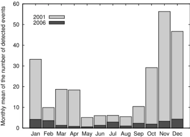
In order to highlight the annual dependence (annual cycle), we focus on two contrasted years: 2001 for the solar maximum and 2006 for solar minimum. Then, the monthly mean of the number of ionospheric events is shown in Figure 2. We can clearly observe that the ionospheric irregularities are more nu-merous during autumn and winter months, even during solar minimum. However, the number of events detected during July 2006 is nearly as large as the number of events detected during winter months. 0 10 20 30 40 50 60
Jan Feb Mar Apr May Jun Jul Aug Sep Oct Nov Dec
Monthly mean of the number of detected events
2001 2006
Figure 2: Annual dependence of the number of detected events
2.2.3 Local time dependence
Ionospheric irregularities also show a local-time dependence that we propose to analyse by dividing local time into 15 min time intervals. For each of them we count the number of ionospheric events detected for 2001 and 2006; the results are shown in Figure 3. We can clearly identify a first maximum of occurrence around 10 A.M. and a secondary maximum during nighttime. However, it is interesting to highlight the fact that the secondary maximum of the low solar activity period (2006) located around 8 P.M. is of the same order of magnitude than the first maximum located around 10 A.M. A similar approach detailed in [2] and which splits this analysis according to the four seasons allows us to distinguish two main types of irregu-larities:
1. autumn/winter irregularities which occur mainly during daytime (around 10 A.M.)
2. summer irregularities which occur mainly during night-time (around 8 P.M.). 0 50 100 150 200 0 4 8 12 16 20 24
Annual sum of detected events
Local time (h) 2001 2006
Figure 3: Local time dependence of the number of detected events
2.2.4 Types of structures detected
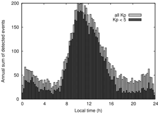
During the climatological analysis (cf. § 2.2.1), we have seen that the number of ionospheric irregularities depends on so-lar activity. In particuso-lar, it is well known that geomagnetic storms, which are more frequently observed during solar ma-ximum, can generate strong variability in TEC. Therefore, it is important to quantify the part due to geomagnetic storms in the statistics described above. In order to isolate this influence, we focus on the days for which the daily maximum Kp value is lower or equal to 5. New statistics are computed on the ba-sis of these “quiet” days in terms of geomagnetic activity using the same procedure as detailed previously. The annual sum of detected events for the year 2001 is shown in Figure 4.
0 50 100 150 200 0 4 8 12 16 20 24
Annual sum of detected events
Local time (h) all Kp Kp < 5
Figure 4: Influence of geomagnetic disturbances on the number of detected events in 2001. This figure shows the annual sum of detected events for each 15 min interval when
considering (light grey) or not (dark grey) the stormy days
We can see that, if we remove from the statistics the days where geomagnetic storms occurred, the shape of the temporal distri-bution remains the same: maxima and minima are still located around the same local time. Therefore, there are two main types of ionospheric irregularities which can be identified:
1. irregularities presenting a monthly and daily dependence. They are due to Travelling Ionospheric Disturbances (TID’s) which present different local-time behaviours ac-cording to the season
2. irregularities which do not show specific local-time be-haviour. These are “noise-like structures” induced by geo-magnetic storms and which are positively correlated with high solar activity periods.
2.3 Quantitative analysis
The climatological study presented in the previous section does not give the magnitude of TEC variability (RoTEC) due to the structures detected by the “one-station” method. Therefore, we propose to extract for the 2001–2007 period the maximum RoTEC values observed for each season at BRUS (Table 1).
Spring Summer Autumn Winter
2001 6.881 1.147 4.028 9.068 2002 0.745 1.821 1.946 2.211 2003 0.693 0.653 9.839 1.231 2004 1.581 1.152 0.861 1.263 2005 1.234 2.579 0.543 1.276 2006 0.582 1.197 0.805 0.845 2007 1.068 0.886 0.593 0.796
Table 1: Maximum RoTEC values from 2001 to 2007 (expressed in TECu)
Table 1 shows that maximum RoTEC values observed during solar minimum (2006 & 2007) are generally lower than during high solar activity periods (2001 & 2002), which confirms the close relationship between solar activity and ionospheric irre-gularities. However, if we consider, for example, only the sum-mer months, we can observe that maximum variability during solar minimum (summers 2005 & 2006) is larger than during solar maximum in 2001. That means that GNSS signals can be significantly disturbed by ionospheric variability, whatever solar activity.
3
Small-scale structures and double differences
As the “one-station” method gives information about the tem-poral gradients of the ionosphere, it does not yield direct infor-mation about spatial gradients between two stations (i.e. for a given baseline). Therefore, we developed a technique which allows to isolate and quantify the ionospheric residual error present in RTK basic observables.3.1 Methodology
RTK basic observables are called “double differences” (DD) and are formed by using data coming simultaneously from two receivers (a reference station and a user station) and two satel-lites. IfϕAi,ϕBi,ϕAj andϕBj are the four “one-way” measure-ments between the receivers A, B and the satellites i, j, the dou-ble differenceϕAB,ki j on Lkcarrier is computed as follows:
ϕi j AB,k = (ϕAi−ϕBi) − (ϕ j A−ϕ j B) = fk c(D i j AB−I i j AB,k+ T i j AB+ M i j AB,k) +NAB,ki j +εAB,ki j (3)
with c the speed of light, Di jABthe geometric term between the different satellites and stations, IAB,ki j the ionospheric residual term, TABi j the tropospheric residual term, MAB,ki j the multipath term, NAB,ki j the ambiguity term andεABi j,kthe noise on the double difference. In our future developments, the ionospheric effects on DD are assessed by using fixed reference stations for which the position is precisely known; as a consequence, Di jAB is a known parameter and is computed by using accurate satellite and station coordinates.
In practice, RTK users measure their position in real-time by using DD of L1and L2phase measurements. Before starting surveying, RTK users must solve integer ambiguities inherent to L1 and L2 double differences. This ambiguity resolution process could fail if the residual ionospheric error contained in the double differences (i.e. IAB,ki j ) is equal or larger than about half a cycle.
Therefore, it is important to quantify the residual ionospheric term in DD, which can be computed by forming the Geometric-Free phase combinationϕAB,GFi j . Considering Equation (3) and neglecting multipath and noise, we obtain:
ϕi j AB,GF = ϕ i j AB,L1− f1 f2ϕ i j AB,L2 [cycles] = 0, 552.10−16STECij AB+ N i j AB,GF (4)
For each double difference observed, the float ambiguity NAB,GFi j is computed by using the data of the entire available duration of the considered satellite pair; in other words, this ambiguity is not a “real-time” ambiguity. Therefore, we are able to compute the ionospheric parameter STECijABand recon-struct the ionospheric residual term on each of the GPS carriers IAB,ki j :
IAB,ki j =40.3
fk2 STEC ij
AB (5)
More details about the method used can be found in [4] and [2].
3.2 Results for case studies
In this study, we analyse the behaviour of IAB,Li j
1 for a
base-line near Brussels; the two stations involved in this basebase-line are GILL and LEEU and are distant of 11 km from each other, which can be considered as a typical baseline length for RTK. In order to clearly identify the effects of ionospheric structures on RTK positioning, we select three days representing typical ionospheric conditions on the basis of the RoTEC values ob-served at BRUS thanks to the one-station method (see § 2):
1. a quiet day in terms of ionospheric activity: DOY 103/07 (April 13th 2007)
2. a day characterised by the occurrence of a medium-amplitude TID: DOY 359/04 (December 24th 2004) 3. a day characterised by the occurrence of one of the most
powerful geomagnetic storm (since the beginning of the GPS system): DOY 324/03 (November 20th 2003). The analysis of all the satellite pairs of the quiet day 103/07 shows that IAB,Li j
1 observations do not show values larger than
0.29 L1cycle, which means that ionospheric effects should not degrade the ambiguity resolution process. The mean of the ab-solute values is about 0.04 L1cycle with a standard deviation of 0.03 L1cycle. These numbers can be considered as the nom-inal conditions for a typical RTK baseline of 11 km.
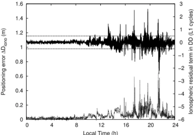
Figures 5 & 6 display the values of the ionospheric residual term IAB,Li j
1respectively for DOY 359/04 and DOY 324/03. We
can observe that geomagnetic storms have a stronger influence on double differences than TID’s: maximum variability value is about 0.9 cycle for DOY 359/04 and 2.6 cycle for DOY 324/03. Moreover, the threshold of 0.5 cycle is slightly exceeded for a small time interval during the occurrence of the TID while it is often reached during the geomagnetic storm.
These results show that small-scale ionospheric variability can represent a threat for GNSS applications, even for differential applications like RTK. This observation is of great importance because RTK users usually assume that residual ionospheric effects can be neglected because of the short distance existing between the user and the reference station.
In the next section, we analyse the effects of such structures on positioning. 0 0.2 0.4 0.6 0.8 1 1.2 1.4 1.6 0 4 8 12 16 20 24−6 −5 −4 −3 −2 −1 0 1 2 3 Positioning error ∆ Diono (m)
Ionospheric residual term in DD (L1 cycles)
Local Time (h)
Figure 5: Ionospheric residual term IABi j,L
1(solid line) and
positioning error∆Diono(dashed line) during the occurrence of
a medium-amplitude TID (DOY 359/04)
0 0.2 0.4 0.6 0.8 1 1.2 1.4 1.6 0 4 8 12 16 20 24 −6 −5 −4 −3 −2 −1 0 1 2 3 Positioning error ∆ Diono (m)
Ionospheric residual term in DD (L1 cycles)
Local Time (h)
Figure 6: Ionospheric residual term IABi j,L
1(solid line) and
positioning error∆Diono(dashed line) during a severe
4
Small-scale structures and GPS-RTK
posi-tioning
This section deals with the ionospheric effects in terms of RTK positioning error. The main objective is to determine the part of the RTK positioning error budget caused by small-scale iono-spheric variability. The same cases as in section 3 have been analysed in the following paragraphs.
4.1 Methodology
In a first step, we select one of the two stations of the baseline and consider it as the user station; the other one will be referred to as the reference station. Then, we compute the three com-ponents (North, East, Height) of the RTK user position every 30 s by using a least-square adjustment of double differences shown in Equation (6): ϕi j AB,k−N i j AB,k= fk c(D i j AB−I i j AB,k+ T i j AB+ M i j AB,k) +ε i j AB,k (6)
In this step, we assume that the ambiguity NAB,ki j has been solved to the correct integer value. As a consequence, the RTK positioning error depends on the unknowns which are mainly the atmospheric errors (troposphere and ionosphere).
Then, we correct the DD of Equation (6) for the ionospheric residual term IAB,ki j which has been computed using Equa-tions (3) & (5): ϕi j AB,k−N i j AB,k+ fk c I i j AB,k= fk c(D i j AB+ T i j AB+ M i j AB,k) +ε i j AB,k (7)
Therefore, we obtain every 30 s a new RTK user position for which the troposphere remains the only major error source. Finally, to isolate the ionospheric influence on positioning er-ror, we compute the difference between the RTK user position obtained from DD corrected and not corrected for the iono-spheric residual term IAB,ki j . Then, we express this positioning error in terms of distance and will refer to this value as∆Diono.
More details about the method used can be found in [3].
4.2 Results for case studies
We analyse the same cases than in section 3.2: three baselines corresponding to each of the three different ionospheric condi-tions previously mentionned.
The results show that, during the quiet day (103/07), the po-sitioning error never exceeds 9 cm, except for a few outliers easily identified. This maximum value is of the same order of magnitude than the nominal accuracy of the RTK position-ing technique which is a few centimetres. The mean value of
∆Dionois 1.6 cm with a standard deviation of 1 cm.
During the occurrence of the TID (DOY 359/04), the position-ing error due to the residual ionosphere reaches 15 cm (Figure 5 – left axis). We can also observe that the variability of the po-sitioning error and of the ionospheric residual term IAB,Li j
1 are
positively correlated. Another small-scale structure detected in IAB,Li j
1 around 18h induced also a large positioning error.
The effects of the severe geomagnetic storm of DOY 324/03 on positioning error are plotted in Figure 6. We can observe that
∆Dionovalues increase at the same time than the variability of
IAB,Li j
1; a maximum value of approximately 65 cm is observed
around 21h30.
It is important to highlight the fact that the positioning errors computed using the above-mentionned methodology are repre-sentative of positioning errors due to the ionosphere encoun-tered by RTK users who have already solved their ambiguities. In case ionospheric disturbances occur during the ambiguity resolution process, the positioning error could reach several meters.
Conclusions
We have seen that small-scale ionospheric structures can in-duce severe degradations of GNSS signals. Such degradations present not only a large variability in time but also a spatial extent. That is the reason why we are studying how these irreg-ularities affect differential applications like RTK. Results sug-gest that geomagnetic storms induce the larsug-gest variability in double differences and, a fortiori, in the RTK error budget, in comparison with other ionospheric structures like TID’s.
Acknowledgements
This research is supported by the Belgian Solar-Terrestrial Centre of Excellence (STCE) and the Belgian Science Policy (BELSPO).
References
[1] R. WARNANT, E. POTTIAUX. "The increase of the iono-spheric activity as measured by GPS", Earth Planets Space, 52, pp. 1055-1060, (2000).
[2] R. WARNANT, G. WAUTELET, J. SPITS, S. LEJEUNE. "Characterization of the ionospheric small-scale activity", Technical report, WP 220, GALOCAD project, contract GJU/06/2423/CTR/GALOCAD (2008).
[3] G. WAUTELET, S. LEJEUNE, S. STANKOV, H.
BRENOT, R. WARNANT. "Effects of small-scale at-mospheric activity on precise positioning", Techni-cal report, WP 230, GALOCAD project, contract GJU/06/2423/CTR/GALOCAD (2008).
[4] S. LEJEUNE, R. WARNANT. "A novel method for the quantitative assessment of the ionosphere effect on high accuracy GNSS applications, which require ambiguity resolution", Journal of Atmospheric and Solar-Terrestrial Physics, 70, pp. 889-900, (2008).