Practical methods for measuring and managing operational risk in the financial sector: A clinical study

Practical Methods for Measuring and Managing Operational Risk in the

Financial Sector: A Clinical Study

Ariane Chapellea Yves Cramab Georges Hübnerc Jean-Philippe Petersd

First version, July 2004. Revised, August 2007 Abstract

This paper analyzes the implications of the Advanced Measurement Approach (AMA) for the assessment of operational risk. Through a clinical case study on a matrix of two selected business lines and two event types of a large financial institution, we develop a procedure that addresses the major issues faced by banks in the implementation of the AMA. For each cell, we calibrate two truncated distributions functions, one for “normal” losses and the other for the “extreme” losses. In addition, we propose a method to include external data in the framework. We then estimate the impact of operational risk management on bank profitability, through an adapted measure of RAROC. The results suggest that substantial savings can be achieved through active management techniques.

Keywords: Operational risk, advanced measurement approaches, extreme value theory, RAROC, risk management

JEL Codes: C15, G20, G21

* _{The authors wish to thank the reviewers and the participants of the 2004 National Bank of Belgium (NBB)} conference on “Efficiency and Stability in an Evolving Financial System”, where a first version of this work was presented, the 2004 Northern Finance Association Conference (St-John’s, Canada), the 2005 Deloitte Conference on Risk Management (Antwerp) and the 2005 Global Finance Association Conference (Dublin) for helpful comments. We thank Fitch Risk for providing us with the FIRST database. Financial support of the NBB is gratefully acknowledged. Part of this research was carried out while Georges Hübner was visiting HEC Montreal; he gratefully acknowledges financial support from Deloitte Luxembourg and a research grant from the Belgian National Fund for Scientific Research (FNRS). This paper was reviewed and accepted while Prof. Giorgio Szegö was the Managing Editor of The Journal of Banking and Finance and by the past Editorial Board. a _{Associate Professor of Finance, Solvay Business School, Université Libre de Bruxelles, Belgium. E-mail:} ariane.chapelle@ulb.ac.be

b _{Professor of Operations Research, HEC Management School, Université de Liège, Belgium. E-mail:} y.crama@ulg.ac.be

c _{Corresponding Author. The Deloitte Professor of Financial Management, HEC Management School, Université} de Liège, Belgium; Associate Professor of Finance, Maastricht University, The Netherlands; and Academic Expert, Luxembourg School of Finance, University of Luxembourg. Address: HEC Management School, University of Liège, Rue Louvrex 14 – N1, B-4000 Liège, Belgium. Tel: (+32)42327428. E-mail: g.hubner@ulg.ac.be

d _{Deloitte Luxembourg, Advisory and Consulting Group (Risk Management Unit), HEC Management School,} Université de Liège, Belgium E-mail: jppeters@deloitte.lu

Practical Methods for Measuring and Managing Operational Risk in the

Financial Sector: A Clinical Study

Abstract

This paper analyzes the implications of the Advanced Measurement Approach (AMA) for the assessment of operational risk. Through a clinical case study of a loss event matrix concerning two business lines and two event types for a large financial institution, we develop a procedure that addresses the major issues faced by banks in the implementation of the AMA. For each cell, we calibrate two truncated distributions functions, one for “normal” losses and the other for the “extreme” losses. In addition, we propose a method to include external data in the framework. We then estimate the impact of operational risk management on bank profitability, through an adapted measure of RAROC. The results suggest that substantial savings can be achieved through active management techniques.

Practical Methods for Measuring and Managing Operational Risk in the Financial

Sector: A Clinical Study

1. Introduction

Since the first Basel Accord was adopted in 1988, the financial sector consistently complained about its simplistic approach based on the Cooke ratio for the determination of regulatory capital. The need for reorganizing the framework under which exposures to credit risk should be assessed was a major impetus for the revision of this system through the second Accord, or Basel II. The Basel Committee on Banking Supervision (hereafter the Basel Committee) seized this opportunity to extend the scope of its proposals by introducing explicit recommendations with regard to operational risk.1

While the two simplest approaches proposed by Basel II (i.e., the Basic Indicator Approach, or BIA, and the Standardized Approach, or SA) define the operational risk capital of a bank as a fraction of its gross income, the Advanced Measurement Approach (AMA) allows banks to develop their own model for assessing the regulatory capital that covers their yearly operational risk exposure within a confidence interval of 99.9% (henceforth, this exposure is called Operational Value at Risk, or OpVaR). Among the eligible variants of AMA, a statistical model widely used in the insurance sector and often referred to as the Loss Distribution Approach (LDA) has become a standard in the industry over the last few years. Yet, the implementation of a compliant LDA involves many sensitive modelling choices as well as practical measurement issues. The first objective of this paper is to develop a comprehensive LDA framework for the measurement of operational risk, and to address in a systematic fashion all the issues involved in its construction.

As a consequence of their conceptual simplicity, BIA and SA models do not provide any insights into the drivers of operational risks, nor into the specific performance of the bank with respect to risk management. By contrast, the LDA model lends itself to quantifying the impact of active operational risk management actions, and justifying (potentially substantial) capital reductions. Unlike credit risk modelling, however, the cost-benefit trade-off of this alternative

approach is largely unknown to date. Therefore, the second major objective of this paper is to examine the costs and benefits associated with two distinct decisions, namely: the adoption of the LDA instead of the basic approaches on one hand, and the improvement of the operational risk management system on the other hand. We propose a RAROC-based framework for the analysis of the financial impact of various operational risk management decisions, where the distribution of losses is viewed as an input and cost variables as an output.

To achieve the two objectives mentioned above, we face most of the practical issues encountered by a financial institution in a similar situation. Namely, in the process of implementing the LDA, the institution must, in turn, (i) infer the distribution of rare losses from an internal sample of observations of limited size, (ii) incorporate possibly heterogeneous external loss data into its estimation, and (iii) account for dependence – or lack thereof – between individual series of losses. Furthermore, the economic analysis of the operational risk management system requires (iv) assessing the impact of managerial actions on the distribution of losses, and finally (v) mapping this loss exposure into an economically meaningful cost function.

The last two issues (iv)-(v) in the above list have apparently not been handled in the literature and require an original investigation. For this purpose, using analogies with credit risk and market risk modelling, we introduce a measure of risk-adjusted return (RAROC) on operational capital and perform a sensitivity analysis based on models developed in the LDA implementation.

By contrast, the first three issues (i)-(iii) in the above list have been previously identified and separately addressed in the financial risk management literature. For instance, Embrechts, Klüppelberg and Mikosch (1997) recommend the use of Extreme Value Theory (EVT) to model the tail of the distribution in risk management, and so do King (2002), Moscadelli (2004), Cruz (2004) or Chavez-Demoulin, Embrechts and Neslehova (2006). Frachot and Roncalli (2002) and Baud et al. (2002) both address the incorporation of external losses in the internal dataset. Applications of copulas to model dependence between financial risks have been reported in the field of market risk, credit risk, insurance or overall risk management, but very few applications seem to have been

performed in the context of operational risk (for an example, see Di Clemente and Romano (2004) or Chavez-Demoulin, Embrechts and Neslehova (2006)). Even so, however, our claim is that these issues cannot be considered as satisfactorily solved from the point of view of operational risk practitioners, since either they have been investigated in a purely theoretical framework (disregarding the inevitable hurdles encountered in any real-world implementation), or, in the best case, they have been addressed as separate and disconnected issues only. As a consequence, methodological gaps remain to be filled in order to link different components of the approach, and practitioners are often at loss when confronted with the formidable task of developing a complete operational risk measurement system based on the LDA.

Our work can be seen as an attempt at overcoming these shortcomings. In the empirical part of our paper, we opt for a clinical case study that encompasses all components of the discussion in a single framework based on real operational loss data collected by a European bank. This methodological choice enables us to adopt the realistic point of view of the risk manager of a specific financial institution. To our knowledge, no published application adopts a similar perspective. The closest work in this respect is a study by Chavez-Demoulin, Embrechts and Neslehova (2006) in which the authors focus on individual statistical modelling issues and illustrate them using transformed operational risk data, a framework which prevents them from discussing the underlying practical issues in great detail. Other related investigations are reported by Fontnouvelle, Jordan and Rosengren (2003), who rely on a public operational loss database (which is not exhaustive and restricted to large losses), and by Moscadelli (2004), who uses loss data gathered during the 2002 Loss Data Collection Exercise carried out by the Basel Committee. The paper by Di Clemente and Romano (2004) performs its analysis on catastrophe insurance data.

The paper is organized as follows. In Section 2 and 3, we discuss the modelling choices underlying the measurement and management of operational risk capital, respectively. Section 4 tests the risk measurement methodology on real data, and assesses the impact of operational risk management on the profitability of the bank. Finally, Section 5 presents some conclusions.

2. Measuring operational risk

2.1. Overview

Although the application of AMA is in principle open to any proprietary model, the most popular methodology is by far the Loss Distribution Approach (LDA), a parametric technique that consists in separately estimating a frequency distribution for the occurrence of operational losses and a severity distribution for the economic impact of individual losses. In order to obtain the total distribution of operational losses, these two distributions are then combined through n-convolution of the severity distribution with itself, where n is a random variable that follows the frequency distribution (see Frachot et al., 2001, for details).

In addition to processing homogeneous categories of internal observations to produce univariate distributions of operational losses for a single type of loss event, the LDA methodology must include two additional steps dealing with different technical issues, namely: integrating external loss data in order to refine the fit of the extreme tail of the distribution; and jointly analyzing the loss event categories, so as to adjust the aggregate distribution for possible dependence between the univariate distributions.2 Sections 2.2, 2.3 and 2.4 respectively describe our implementation of each of these three steps.

The output of the LDA methodology is a full characterization of the distribution of annual operational losses of the bank. This loss distribution contains all relevant information for the computation of the regulatory capital charge – defined as the difference between the 99.9% percentile and the expected value of the distribution – as well as necessary inputs for the assessment of the efficiency of operational risk management procedures.

2.2. Processing of internal data

In this section, we discuss the methodological treatment of a series of internal loss data for a single category of risk events in order to construct a complete probability distribution of these losses.

The frequency distribution models the occurrence of operational loss events within the bank. Such a distribution is by definition discrete and, for short periods of time, the frequency of losses is

often modelled either by a homogenous Poisson or by a (negative) binomial distribution. The choice between these distributions is important as the intensity parameter is deterministic in the first case and stochastic in the second (see Embrechts, Furrer and Kaufmann, 2003).

When modelling the severity of losses, on the other hand, our preliminary tests3 indicate that classical distributions are unable to fit the entire range of observations in a realistic manner. A study by Fontnouvelle et al. (2004) independently reaches similar conclusions. Hence, as in King (2001), Alexander (2003) or Fontnouvelle et al. (2004), we propose to distinguish between ordinary (i.e., high frequency/low impact) and large (i.e., low frequency/high impact) losses originating, in our view, from two different generating processes. The “ordinary distribution” includes all losses in a limited range denoted [L;U] (L being the collection threshold used by the bank), while the “extreme distribution” generates all the losses above the cut-off threshold U. We then define the severity distribution as a mixture of the corresponding mutually exclusive distributions.4

2.2.1. Severity distribution – ordinary losses

The distribution of ordinary losses can be modelled by a strictly positive continuous distribution such as the Exponential, Weibull, Gamma or Lognormal distribution. More precisely, let f(x;θ) be the chosen parametric density function, where θ denotes the vector of parameters, and let F(x;θ) be the cumulative distribution function (cdf) associated with f(x;θ). Then, the density

function f*(x;θ) of the losses in [L;U] can be expressed as

( )

₍

( )

₎

_{( )}

corresponding log-likelihood function is

( )

₍

(

_{) ( )}

)

∑

where (x1,…,xN) is the sample of observed ordinary losses. It should be maximized in order to estimate θ.

2.2.2. Severity distribution – large losses

Small-sized samples containing few – if any – exceptional, very severe losses represent a common issue when dealing with operational losses in banks (see Embrechts et al., 2003). When applied to such samples, classical maximum likelihood methods tend to yield distributions that are not sufficiently heavy-tailed to reflect the probability of occurrence of exceptional losses. To resolve this issue, we rely on concepts and methods from Extreme Value Theory (EVT), and more specifically on the Peak Over Threshold (POT) approach. This approach will enable us to simultaneously determine the cut-off threshold U and to calibrate a distribution for extreme losses using all the observations above this threshold.

The procedure builds upon results of Balkema and de Haan (1974) and Pickands (1975) which state that, for a broad class of distributions, the values of the random variables above a sufficiently high threshold U follow a Generalized Pareto Distribution (GPD) with parameters ξ (the shape index, or tail parameter), β (the scale index) and U (the location index). The GPD can thus be thought of as the conditional distribution of X given X > U (see Embrechts et al., 1997, for a comprehensive review). Its cdf can be expressed as:

(

)

While several authors (see e.g. Drees and Kaufmann, 1998, Dupuis, 1999, Matthys and Beirlant, 2003) have suggested methods to identify the cut-off threshold, no single approach has become widely accepted, yet. A standard technique is based on the visual inspection of the Mean Excess Function Plot (see Embrechts et al., 1997, for details). We replace this graphical tool by an algorithmic procedure that builds on ideas from Huisman et al. (2001) and shares some similarities with a procedure used by Longin and Solnik (2001) in a different context. The steps are:

1. Let (x1,…,xn) be the ordered sample of observations. Consider m candidate thresholds U1,…,Um

2. For each threshold Ui, use the weighted average of Hill estimators proposed by Huisman et al.

(2001) to estimate the tail index ξi of the GPD distribution.

3. Compute the maximum likelihood estimator of the scale parameter βi of the GPD, with the tail

index ξi fixed to the value obtained in step 2.

4. For each threshold Ui, compute the Mean Squared Error statistic5

∑

(

)

= − = ni k k k i i F F n U MSE 1 2 ˆ 1 ) ( ,

where ni is the number of losses above threshold Ui, Fk is the cdf of the GPD(ξk,βk,μ k) and

is the empirical cdf of the excesses.

k Fˆ

5. Identify MSE(Uopt) = min(MSE(U1),…,MSE(Um)); is retained as estimator of the cut-off

threshold and the excesses are assumed to follow a Uˆ

(

)

GPDξˆ,βˆ, ˆ distribution.

Note in particular that the method proposed in Step 2 corrects for the small-sample bias of the original Hill estimator. As the robustness of maximum likelihood estimators might be questioned when working with very small dataset, we prefer to rely on this modified Hill estimator to fully benefit from the information contained in the whole dataset. As a consequence, however, the estimation of the tail and scale parameters requires two successive steps (namely, Steps 2 and 3).

2.3. Processing of external data

In order to comply with Basel II, the AMA ought to specify a proper way to integrate external loss data into the capital charge calculation using one of the following three methods: • integrating external data in the internal loss database to increase the number of observations; • separately estimating the operational risk profile of internal and external database and

combining them by Bayesian techniques (see Chapter 7 in Alexander, 2003);

• providing additional examples and descriptions of real large loss events to illustrate “what if” scenarios and to allow the self-assessment of extreme risks.

In this study, we illustrate a possible implementation of the first option. Keeping in line with the recommendations of the Basel Committee (2004), we use an external dataset of very large losses

in order to improve the accuracy of the tail of the severity distribution6. (Note that, by contrast, Frachot et al., 2002, create an enlarged sample containing a mix of internal and external data that cover losses of all sizes).

As observed by Frachot and Roncalli (2002) and Baud et al. (2002), integrating external data in the internal loss database raises major methodological questions, including the determination of an appropriate scaling technique which allows to account for the size of the bank (see also Shih et al., 2000, Hartung, 2003). To scale the external severity data, we follow the approach of Shih et al. (2000) and we accordingly posit the non-linear relationship:

, r S

Loss= a (3)

where Loss is the magnitude of the loss, S is a proxy for the firm size (its gross income, in our implementation7), a is a scaling factor, and r is the multiplicative residual term not explained by any fluctuations in size. Note that if a = 0, the severity of the losses is not related to the size of the institution. If a = 1, this relation is assumed to be linear.

Equation (3) yields the linear regression model

i i i i S b a S Loss _ε + + = ) ln( 1 ) ln( ) ln( (i = 1,…p) (4)

where (Lossi,Si), i = 1,…p, are the external observations. This model can be estimated by OLS.

Then, the scaled loss Lossiscaled associated to observation i can be computed as a i int i scaled i S S Loss Loss _⎟⎟ ⎠ ⎞ ⎜ ⎜ ⎝ ⎛ = , (5)

where int is the size of the internal business segment corresponding to observation i. S

By applying the same scaling coefficient a to the collection threshold of the external database, we obtain the threshold E from which the tail of the distribution of internal data is replaced by the calibrated distribution of external data. Finally, a parametric distribution on [E,+∝) can be fitted to the sample of scaled loss data. This will be illustrated in Section 4.2.5 hereunder.

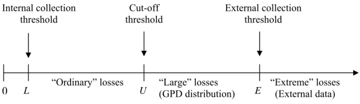
We end up with a distribution of loss severity consisting of three distinct parts, associated respectively with ordinary losses, large losses and extreme losses (see Figure 1). In a simulation framework, this distribution can be sampled by weighing each part of the distribution according to the relative occurrence of each type of losses in the internal loss database.

Insert Figure 1 approximately here 2.4. Dealing with all business lines and event types

The methodology outlined in Sections 2.2-2.3 is applicable to a homogeneous category of operational loss data. In contrast, however, Basel II requires taking into consideration 56 categories of risks, corresponding to 8 business lines and 7 loss events types. For this purpose, the Accord proposes to compute the total capital charge by simple addition of the capital charges for all 56 risk categories, thus implicitly assuming perfect positive dependence between risks. Banks are nevertheless offered the possibility to account for dependence by appropriate techniques.

Dependence between risks can be modelled either between frequencies of loss events, or between their severities, or between aggregate annual losses. Frachot et al. (2004) argue convincingly that “the correlation considered by the Basel Committee is unambiguously the aggregate loss correlation” and that it can be expected to be rather weak in general. They also explain that this dependence can be adequately captured in the LDA framework by the frequency correlations, not by severity correlations (see Frachot et al., 2003, for a discussion of this topic).

We directly model the dependence of aggregate losses through the use of copulas (see e.g. Genest and McKay, 1986, or Nelsen, 1999 for an overview) in order to combine the marginal distributions of different risk categories into a single joint distribution. This method possesses more attractive theoretical properties than traditional linear correlation when dealing with non-elliptical distributions, such as those encountered in operational risk modelling.

If Fi(xi) denotes the marginal cdf of aggregate losses for cell i (i = 1,…, p) of the (business

line×risk type) matrix, then we represent the joint distribution of aggregate losses as where C is an appropriate copula. We report here results , )) x ( F ),..., x ( F C( ) , x , x ( F ₁… ₅₆ = _{1 1 56}

obtained with a mixture copula combining the default Basel II assumption of perfect dependence between risks (corresponding to the upper Fréchet bound) with a much less conservative view, namely, independence between risks.

In its bivariate form, the mixture copula used in this study can be expressed as

(

)

( )

( )

C_θ = 1−θ ⋅ ⊥ , +θ⋅ + , (6)

where θ is the Spearman rank correlation coefficient which is assumed to be positive; un is the cdf

of a uniform U(0,1) distribution; C⊥ denotes the independence, or product, copula defined as

, and C

∏

+ _{denotes the full dependence, or upper Fréchet bound, copula defined as}

. It is often referred to as the linear Spearman copula and is similar to family B11 in Joe (1997) (see e.g. Hürlimann, 2004a,b, for applications to insurance problems).

(

)

8

3. Managing operational risk

Operational risk management involves an array of methods and approaches that essentially serve two purposes: reduction of average losses and avoidance of catastrophic losses. Some of these techniques aim at reducing the magnitude of losses, some at avoiding loss events, some at both.

Table 1 reviews a number of illustrative management actions and three different possible types of impact on the parameters of the loss distributions, either in frequency or in severity: reduction in the number of large losses, reduction in the frequency of all losses, or reduction in the severity of all losses. The business lines or event types impacted depend on the action taken.

Insert Table 1 approximately here 3.1. Mapping of the distribution of losses on profitability

Our methodology produces the necessary tools to estimate the quantitative impact of various risk management actions on the risk-adjusted return of activities, and, in turn, their consequence on the tariffs applicable to financial products.

Remember that RAROC, the Risk Adjusted Return on Capital, is a performance measure that expresses the return of an investment, adjusted for its risk and related to the economic capital consumed when undertaking this investment. The general formula for RAROC writes:

Capital Economic Losses Expected venues Re RAROC= − (7)

The adjustment for risk takes place both in the numerator and the denominator of the ratio. Until recently, the RAROC performance measure had been mostly used to assess the credit activities of banks. Since the Basel Accord introduces regulatory capital for operational risks, banks could start considering introducing risk-adjusted pricing of activities that are particularly exposed to operational risk and developing an analogous RAROC approach to operational risk. In order to obtain a proper RAROC measurement adapted to operational risk, we must identify (i) expected losses due to operational events; (ii) economic capital necessary to cover the unexpected operational losses; and (iii) revenues generated by taking operational risks.

The first two inputs are readily derived from our methodology, as the fitted distribution of operational losses provides both the expected aggregate loss and the percentile for the regulatory 99.9% OpVaR used to determine regulatory capital. The estimation of the revenues associated with operational risks represents a more complex challenge. Unlike credit risk whose counterpart in revenues can be clearly identified, we face here the fundamental question of the existence of operational revenues as counterpart of operational risks. Strictly speaking, operational revenues are null. We plead for a less restrictive view, though, since even pure market or credit activities, and a fortiori those that generate other types of revenues like the fee business (asset management, private banking, custody, payments and transaction) involve large components of business and operational risks that call for compensation through an adequate tariff policy. A proportion of the bank revenues are generated by operations and are, as such, a counterpart for operational risk. Along the same line of reasoning, banks are willing to apply a mark-up to the price of their operations, in order to get a

proper remuneration for the operational risk they generate by doing business. As a first approximation, this mark-up is equal to the gross operating margin of the financial institution.

Thus we define the “operational” RAROC (RAROCO) of a business line i as

. ) i ( Capital Economic ) i ( EL ) i ( GI ) i ( RAROCO op op op − = (8)

Here, GIop(i) = λi × GI(i) where GI(i) is the Gross Income of business line i and λi is the mark-up for

operational risks charged by business line i (equal to its gross operating margin). The choice of a multiplier of gross income is justified by the evolution of financial institutions towards an adaptation of their tariffs in consideration with the Basel II Accord.

The formulation in equation (8) allows us to perform two kinds of economic analyses: first, we can directly quantify the impact of a given management action on the RAROCO, generated by the reduction of EL and the subsequent variation of economic capital following better risk management. Second, the specification of a target value for the RAROCO induces estimates of the maximum acceptable cost of a given action through the variation of the necessary level of revenues to maintain the target RAROCO.

4. Empirical analysis

4.1. Data

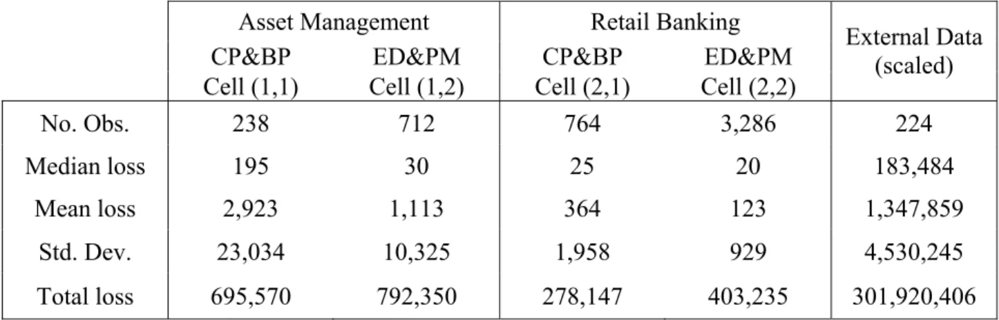
The methodology outlined in Sections 2 and 3 has been applied to real operational loss data provided by a large European bank. Data collection has been performed in compliance with the Basel II definition of business lines and event types, but the available data set is still incomplete and unsatisfactory in some respects. Therefore, and since our main purpose is to illustrate a methodology (and not to analyze the exact situation of a specific institution), we focus our analysis on a sub-matrix consisting of two rows and two columns of the original (business lines × loss event) matrix. The selected business lines are “Asset management” and “Retail banking”, while the loss event types are “Clients, products & business practices” and “Execution, delivery & process

management”. For the sake of data confidentiality, we have multiplied all loss amounts by a constant and we have adjusted the time frame of data collection so as to obtain a total of 5,000 loss events.9 Summary statistics are given in Table 2.

Our external data set is the OpVar Loss Database provided by Fitch Risks. It consists of publicly released operational losses above USD 1 million collected by the vendor. We have filtered the database to remove losses arising from drastically different geographical regions and/or activities. Moreover, in order to allow scaling (see Section 2.3), we keep losses only from those banks whose gross income is available in the database. The summary statistics of external losses are provided in Table 2.

Insert Table 2 approximately here 4.2. Calibration of LDA

4.2.1. Frequency distribution

We illustrate the computation of the Operational Value-at-Risk (OpVaR) for the cell “Asset Management / Execution, process and delivery management” (henceforth Cell (1,2)).

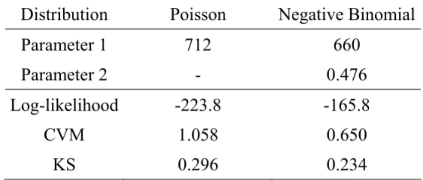
The variance of the monthly frequency series is higher than its mean, suggesting that a negative binomial distribution might be more appropriate than a Poisson process. This is confirmed by Table 3, which displays some classical goodness-of-fit measures that all favour the negative binomial distribution against the Poisson distribution.

Insert Table 3 approximately here

For Cell(1,2), the fitted frequency distribution is a Negative Binomial (645, 0.459). 4.2.2. Internal data

Applying the algorithm developed in section 2.2.3, the weighted average of Hill estimators proposed by Huisman et al. (2001) is ξ = 1.412. The subsequent steps of this algorithm yield the optimal cut-off threshold U = 537 (64 loss events exceed this threshold). Using a constrained Maximum Likelihood approach to estimate the remaining parameter of the GPD, we obtain β = 994.2. Thus we

conclude that the extreme losses of the sample (above the threshold U = 537) are modelled by a GPD with tail index ξ = 1.412, scale index β = 994.2 and location index U = 537.

Insert Table 4 approximately here

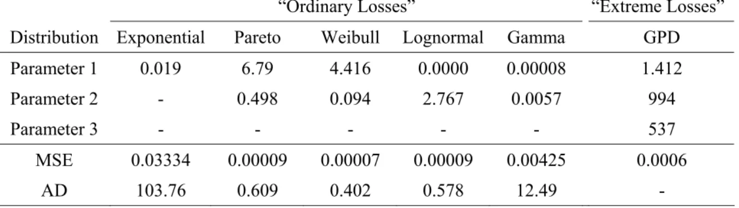
To fit the distribution of the “ordinary” losses (smaller than U = 537), we calibrate five distributions10 (Exponential, Pareto, Weibull, Lognormal and Gamma) by maximizing the log-likelihood expression in equation (1). A summary of the different fitting exercises is given in Table 4. In each case, we report the Mean Squared Error and Anderson-Darling goodness-of-fit indicators (adapted to account for the truncation of the distributions). The Weibull distribution with parameters a= 4.42 and b= 0.094 provides the best fit for this specific cell.

4.2.3. Measurement for the complete matrix

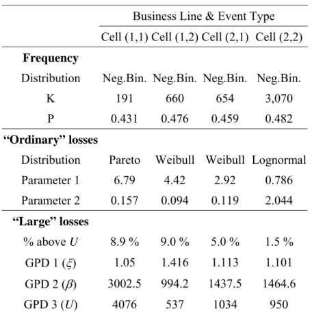
A similar methodology has been used for the other three cells of the matrix. Table 5 summarizes the corresponding results. If the operations of the bank were limited to these four cells, Table 6 would directly provide the total required capital charge for operational risk under the assumption of perfect dependence between the cells of the matrix and without inclusion of external data.

Insert Table 5 approximately here

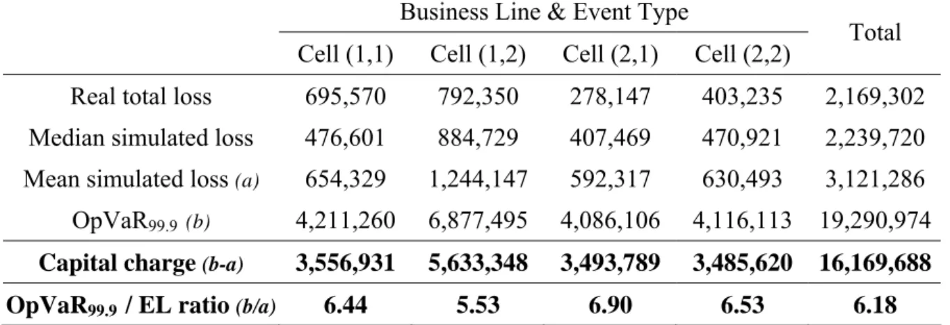
Based on the default assumption of Basel II, we simply need to aggregate the OpVaR in excess of Expected Losses to get the overall capital charge. Table 6 indicates that the total capital charge (estimated by Monte Carlo simulation) amounts to:

19.29 million (OpVaR99.9) – 3.12 million (Expected Loss) = 16.17 million.11 Insert Table 6 approximately here

4.2.4. Dependence

We now turn to the explicit introduction of a dependence structure among risks. With a sample of limited extent, one can only perform reliable inference about dependence by analyzing weekly or monthly observations. However, in order to carry out the OpVaR calculations, we would really need to identify the dependence structure between aggregated yearly losses. In order to work around this difficulty, we make the following observation: under the i.i.d. assumption for monthly

losses relating to a single class of risk (i.e., for an individual cell of the loss matrix), there does not exist any non-contemporaneous dependence between observations relating to different classes of risks (i.e., to different cells), and the observed dependence structure at the monthly level can simply be transposed at the yearly level.12 To assess whether this transposition can actually be performed, we have run a Vector AutoRegressive (VAR) analysis on the monthly aggregated losses. Our results indicate that almost no coefficient is significant at the usual confidence level. Therefore, we use the monthly dependence structure in our annual simulations.

Insert Table 7 approximately here

Table 7 displays the Spearman’s rank correlation coefficients13 between monthly aggregate losses of the four cells. The relatively low values of these coefficients confirm that the perfect positive dependence assumption appears unduly strong. Taking the “real” dependence structure into account would lead to more accurate results and possibly lower the total required capital charge (as predicted by Frachot et al., 2004).

Due to data availability reasons, some banks might not be able to calibrate the copulas modelling the dependence structure between individual cells. A solution to this problem is to concentrate instead on the dependence between business lines, conservatively assuming perfect positive dependence between loss event types. To assess the impact of such an assumption, Table 8 also provides estimations obtained when using “real” dependence between business lines only. Spearman’s correlation coefficient between the aggregate losses of the two business lines under consideration is equal to 0.042. As this value is also the weight associated with the upper Fréchet copula (corresponding to perfect dependence) in Equation (6), this result clearly indicates that the default assumption of Basel II is far from being observed in this clinical study.

Table 8 displays the OpVaR values and the capital charges reported under various dependence assumptions when using the linear Spearman copula to introduce dependence in our Monte Carlo simulations.14 Parameters of the copulas are estimated through a Maximum Likelihood approach and the Monte Carlo experiments are based on a procedure described in Nelsen (1999).As

in the full dependence case, we simulate 20,000 years of losses to obtain the annual aggregated loss distribution for the bank.

Insert Table 8 approximately here

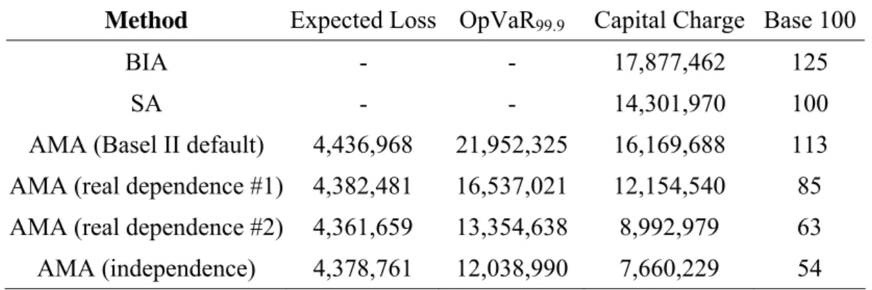
The capital charge obtained with the SA is low when compared to the default AMA, mostly due to the nature of our dataset.15 Taking partial dependence into account substantially reduces the required capital charge with respect to the default AMA, by a factor of about 30%. This is consistent with results reported in the literature (for instance, Frachot et al. (2001) report potential reductions of 38% for the capital charge while Chavez et al. (2006) observe a decline of slightly more than 40% when comparing full independence with perfect dependence on a 3-business lines example).In this study, if the costs associated with the adoption of an advanced measurement approach (IT systems to collect, store and handle data, training costs for staff, potential need for skilled resources to maintain the model, etc.) represent less than 38% of the capital charge under SA, it may be worthwhile adopting the AMA on an own funds requirements basis.

4.2.5. External data

To illustrate a possible way to integrate external data in the internal database, we scale the external data described in Table 2 by the procedure of Shih et al. (2000), as explained in Section 2.3. The estimation of equation (4) by OLS regression yields an estimate of the scaling factor a = 0.154 for the external data of Cell (1, 2), which is in line with the findings in Shih et al. (2000) of a highly nonlinear relationship between losses and size. Then we scale the external data accordingly and estimate the distribution of the resulting data. Using the same parametric distributions as in Section 4.2.1, a lognormal distribution (12.37; 1.57) provides the best fit. The rescaled threshold for external losses is E = 21,170.

Next, we can compute the aggregate loss distribution based on a severity distribution that combines three elements: a distribution for the body of the data (“high frequency/low severity” events), the GPD distribution for large losses and the external data distribution for extremely large losses. In order to assess the impact of the introduction of external data on the estimates of the high

percentiles of the aggregate loss distribution and of the regulatory capital, Table 9 provides a comparison between results obtained with or without external data.

Insert Table 9 approximately here

Replacing EVT estimates of the GPD parameters for the very far end of the severity distribution by the fitted distribution of comparable external observations alters the aggregate loss distribution. The mean loss increases with the inclusion of external data, while the tail appears to be thinner. Thus, adding external data results in a more dense distribution of aggregated losses.

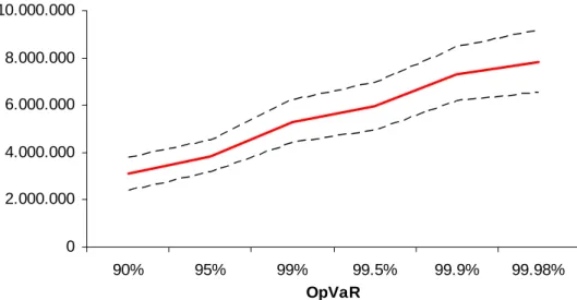
To check the robustness of these results, we report confidence intervals for our estimates derived from a bootstrap analysis. We randomly extract from our internal data a sub-sample containing 90% of the original loss events. Then we estimate the severity distribution of this sub-sample (both the “body” and the “tail” parameters) following the methodology described in Section 2. Finally we derive the aggregated loss distribution (using the same frequency distribution in all cases) and compute the statistics of interest. This process is repeated 250 times. Figures 2a and 2b display the graphical evolution of the confidence intervals.

Insert Figures 2a and 2b approximately here

For the higher quantiles, the confidence intervals have similar sizes for both approaches. However, for smaller quantiles, the confidence interval tends to be narrower and the median estimate is in general closer to the lower bound of the interval when no external data is used. Apparently, the use of EVT to fit the tail of the loss distribution results in a right-skewed distribution of the quantile estimates.

4.3. Impact of ORM on the RAROC

4.3.1. Determination of the Operational RAROC

The quantitative analysis described in the previous sections provides two out of the three data elements needed to calculate the Operational RAROC (RAROCO), namely, the Expected Loss and the Economic Capital; see Equation (8). The third element, i.e., revenues can be estimated according to two approaches discussed below.

The first approach is to consider that a proportion of the bank revenues are generated by operations and are, as such, a counterpart to operational risk. For the sake of illustration, we calculate the RAROCO of each of the two business lines according to this view. To quantify the “operational revenues”, we assume that the ratio between expected operational losses and operational revenues is similar to the average cost/revenue ratio in the business line, i.e., the gross operating margin. Our dataset displays an average gross operating margin of 14.0% over the last years for the retail segment, which includes both retail banking and asset management.

The second option is to assess the minimum level of revenue needed in a business line to reach a RAROCO threshold. A common RAROC threshold in the banking industry is 18%, which roughly corresponds to 12% of net ROE, after taking into account tax deductibility since RAROC is a gross return measure. This enables us to compute the minimum compensation level of income which is necessary for the different business lines. More importantly, this view will allow computing the maximum acceptable cost for risk management actions, as detailed in the next sub-section. Results are displayed in Table 10

Insert Table 10 approximately here

Note that the RAROCO values are very low (less than 3.5% with the default AMA). This result indicates that the operational risk-reward relationship does not yield a profitable rate of return for the bank, i.e. it can be seen as a cost center if the bank charges the same gross margin as for the other activities. Nevertheless, the differential results obtained with managerial actions will indicate to what extent they are likely to increase the bank’s profitability.

For both measures, the correction for dependence in the RAROC displays a great improvement over the full dependence case by showing an increase of more than 50% in risk-adjusted return on capital.

4.3.2. Comparative analysis of different risk mitigating actions

We analyze the impact of risk mitigating actions on profitability by comparing the first two actions described in Table 1. For “Dashboards”, the expected frequency of events is proportionally

reduced across all business lines and loss event types while with “Audit Tracking”, the expected frequency and the magnitude of the severity are simultaneously reduced in all business lines for one specific loss event type.

We assume the bank’s management has set the following objectives: (i) to reach a target RAROCO of 18%, and (ii) to reduce the Expected Loss (EL) by 15% for strategic purposes. The risk manager should select the most attractive solution through a cost-benefit analysis.

To solve this problem, we first assess the performance (i.e., the necessary reductions in frequency x and severity y) required for each action in order to reach a 15% reduction of the EL. Next, we combine these performance requirements with the constraint on the target RAROCO to measure the maximum acceptable cost for each action. Table 11 summarizes the impact of the various risk management actions on the inputs of the bank’s profitability.

Insert Table 11 approximately here

Note that different actions, while leading to the same reduction of the expected losses, have different impacts on the unexpected loss and thus on the regulatory capital. Data show that actions targeting Cell (2,2) “Retail banking / Execution, delivery & process management” have the greatest impact on EL. By contrast, Cell (1,2) “Asset management / Execution, delivery & process management” is least impacted by risk management actions.

Overall, the impact on regulatory capital seems to be influenced by two factors: the cell where the effort is targeted, with a dominant impact of Cell (2,2), and the relative focus on severity. From Table 5, Cell (1,2) displays the largest proportion of “Large” internal losses. Thus, any managerial action addressing this cell results in a greater effect on the tail of the distribution.

On the other hand, the variation in unexpected loss, and thus the impact on the regulatory capital, is connected to the relative weight of changes in frequency and severity of losses. For any given cell, a shift from a reduction of frequency of losses to a decrease in severity induces a further reduction in regulatory capital.

Table 12 provides an overview of the major results ensuing from a successful implementation of these actions. The “Acceptable Cost” column indicates the percentage of income that can be spent to implement the risk management action while maintaining the same RAROCO level for the activity.

Insert Table 12 approximately here

In all cases, by reducing the EL and the Economic Capital, operational risk management measures improve the RAROCO performance of the business lines to a significant extent. The RAROCO doubles (for dashboards) and almost triples (for audit tracking actions) after completion of the management actions.

The objective of loss reduction subject to the profitability constraint is achieved if the performance requirements on frequency and severity described above are met. A cost-benefit analysis is needed to ensure that the costs associated with their implementation do not exceed the benefits that they carry. Accordingly, Table 12 reads as follows: if the costs linked to an “Audit tracking” plan allowing a reduction of 12% of the number of losses per year and a 5% reduction of their severity (see Table 10) represent less than 0.98% of the cumulated Gross Income of the two business lines, then the management’s objectives (15% reduction of Expected Loss and a target RAROCO of 18%) are met.

Our approach permits to compare acceptable costs between different managerial actions. In our case, thanks to its better impact on economic capital reduction, cost incurred by the implementation of “Audit Tracking” action can be substantially greater than for “Dashboards” while still meeting the managerial wishes described above.

5. Concluding remarks

In this paper, we have attempted to explicitly and consistently address several major issues triggered by the emergence of operational risk coverage in the scope of the Basel II Accord. The first part of the paper is rooted in the observation of a significant gap between theoretical

quantitative approaches in the academic literature and the somewhat pragmatic approaches to modelling of operational losses adopted in the banking industry. We believe that this gap is due to the practical difficulties met in the implementation of advanced theoretical models. Thus, a first objective of our work was to suggest and implement a complete methodological framework to overcome these difficulties, whose various steps have been illustrated on a realistic case-study.

As for the next research question, namely the cost-benefit analysis of adopting the AMA instead of a less sophisticated method, two major conclusions can be drawn. First, the behaviour of extremely large losses collected in external databases, as well as the dependence structure of operational losses among business lines and/or event types, are both likely to affect the cost-saving properties of the AMA choice in a significant way. A proper treatment of external data allows refining the analysis of the tail of the aggregate loss distribution. Furthermore, since the AMA aims at capturing rare events, it tends to be overly conservative when the basic assumption of additive capital charges (perfect correlation) is adopted. The estimation of risk exposure is significantly reduced when dependence is taken into account in a reasonable way.

Second, the differential capital charge between the Standardized Approach and the AMA, and thus the opportunity cost of adopting (or not) a complex operational risk management system, significantly hinges on the discretionary weight assigned to the business lines. Banks should not take capital reduction for granted when adopting well-calibrated AMA, as the choice of the SA may be attractive to some banks whose risk is greater than average, and unattractive to others. With this respect, our cost-benefit trade-off analysis of adopting a full-fledged operational risk management system has less normative content than methodological substance. On the basis of controlled scenarios, we document that managerial actions are likely to bring significant improvements on the risk-adjusted profitability of the institution. The arbitrage between different managerial actions is mostly tied to the distributional behavior of the aggregate loss for each business line and event type. This kind of analysis of the profit side of operational risk management should be matched with a

more industrial view on the cost-side of these types of actions, which is beyond the scope of the study.

All aspects of this research could be extended in various ways provided more complete and robust databases would become available. For instance, the inclusion in the framework of “soft” elements such as experts’ opinion, or bank-specific business environment and internal control factors, remains a major methodological challenge.16 This very promising area will actually reach its full potential only when banks will have collected extensive operational data – both on loss events and on corrective devices – on a systematic basis for several years.

References

Alexander, C., 2003. Operational Risk: Regulation, Analysis and Management. FT Prentice Hall, London.

Allen, L., Bali, T.G., 2005. Cyclicality in catastrophic and operational risk measurements. Working paper.

Balkema, A.A., de Haan, L., 1974. Residual life time at great age. Annals of Probability 2, 792-804.

Bank of America, 2003. Implementing a comprehensive LDA. Proceedings of the "Leading Edge Issues in Operational Risk Measurement" Conference. New York Federal Reserve.

Basel Committee on Banking Supervision, 2003. Sound practices for the management and supervision of operational risk. Bank for International Settlements, Basel.

Basel Committee on Banking Supervision. 2004. Basel II: International convergence of capital measurement and capital standards – A revised framework. Basel Committee Publications No. 107, The Bank for International Settlements, Basel.

Baud, N., Frachot, A., Roncalli, T., 2002. Internal data, external data and consortium data for operational risk measurement: How to pool data properly. Working Paper, Groupe de Recherche Opérationnelle, Crédit Lyonnais..

Chavez-Demoulin, V., Embrechts, P., Neslehova, J., 2006. Quantitative models for operational risk: extremes, dependence and aggregation. Journal of Banking and Finance 30, 2635-2658. Cherubini, U., Luciano, E., Vecchiato, W., 2004. Copula Methods in Finance. Wiley & Sons, New York.

Clayton, D. G., 1978. A model for association in bivariate life tables and its application in epidemiological studies of familial tendency in chronic disease incidence. Biometrika 65, 141-151. Cruz, M. G., 2002. Modeling, Measuring and Hedging Operational Risk. Wiley & Sons, New York.

Cruz, M. G. (eds), 2004. Operational Risk Modelling and Analysis: Theory and Practice. Risk Waters Group, London.

Di Clemente, A., Romano, C., 2004. A copula - Extreme Value Theory approach for modelling operational risk, in: Cruz, M. (Ed.), Operational Risk Modelling and Analysis: Theory and Practice, Risk Waters.

Dupuis, D. J., 1999. Exceedances over high thresholds: A guide to threshold selection. Extremes 1 251-261.

Embrechts, P., Furrer, H., Kaufmann, R., 2003. Quantifying regulatory capital for operational risk. Working Paper, RiskLab, ETH Zürich.

Embrechts, P., Klüppelberg, C., Mikosch, T. 1997. Modelling Extremal Events for Insurance and Finance. Springer Verlag, Berlin.

Embrechts, P., Lindskog, F., McNeil, A., 2001. Modelling dependence with copulas and applications to risk management. Working Paper, ETH Zürich.

Embrechts, P., McNeil, A., Strautmann, D., 2002. Correlation and dependence in risk management: Properties and pitfalls,.in Dempster, M.A.H. (Ed.): Risk management: Value at risk and beyond. Cambridge University Press, Cambridge.

de Fontnouvelle, P., Jordan, J., Rosengren, E., 2003. Using loss data to quantify operational risk. Working Paper, Federal Reserve Bank of Boston.

de Fontnouvelle, P., Rosengren, E., Jordan, J., 2004. Implications of alternative operational risk modeling techniques. Working Paper, Federal Reserve Bank of Boston.

Frachot, A., Georges, P., Roncalli, T., 2001. Loss distribution approach for operational risk. Working Paper, Groupe de Recherche Opérationnelle, Crédit Lyonnais.

Frachot, A., Moudoulaud, O., Roncalli, T., 2003. Loss distribution approach in practice. Working Paper, Groupe de Recherche Opérationnelle, Crédit Lyonnais.

Frachot, A., Roncalli, T., 2002. Mixing internal and external data for managing operational risk. Working Paper, Groupe de Recherche Opérationnelle, Crédit Lyonnais.

Frachot, A., Roncalli, T., Salomon, E., 2004. The correlation problem in operational risk. Working Paper, Groupe de Recherche Opérationnelle, Crédit Lyonnais.

Frank, M. J., 1979. On the simultaneous associativity of F(x,y) and x+y-F(x,y). Aequationes Mathematicae 19, 194-226.

Frey, R., McNeil, A.J., Nyfeler, M.A., 2001. Copulas and credit models, RISK, October, 111-114. Genest, C., McKay, J., 1986. The joy of copulas: Bivariate distributions with uniform variables. The American Statistician 40, 280-283.

Gumbel, E. J., 1960. Distributions des valeurs extrêmes en plusieurs dimensions. Publications de Institut de Statistique de l’Université de Paris 9, 171-173.

Hartung, T., 2003. Considerations to the quantification of operational risks. Working Paper, University of Munich.

Hougaard, P., 1986. A class of multivariate failure time distributions. Biometrika 73 671-678. Huisman, R., Koedijk, K. G., Kool, C.J., Palm, F., 2001. Tail-index estimates in small samples. Journal of Business & Economic Statistics 19, 208-216.

Hürlimann, W., 2004(a), Fitting bivariate cumulative returns with copulas. Computational Statistics and Data Analysis 45, 355-372.

Hürlimann, W., 2004(b), Multivariate Fréchet copulas and conditional value-at-risk. International Journal of Mathematics and Mathematical Sciences 7, 345-364.

Industry Technical Working Group on Operational Risk, 2003. Proceedings of the “An LDA-Based Advanced Measurement Approach for the Measurement of Operational Risk: Ideas, Issues and Emerging Practices”, Proceedings "Leading Edge Issues in Operational Risk Measurement" Conference. New York Federal Reserve.

Këllezi, E., Gilli, M., 2003. An Application of Extreme Value Theory for Measuring Risk. Working Paper, University of Geneva.

Longin, F., Solnik, B., 2001. Extreme correlation of international equity markets. Journal of Finance 56, 649-676.

Matthys, G., Beirlant, J., 2003. Estimating the extreme value index and high quantiles with exponential regression models. Statistica Sinica 13, 853-880.

McNeil, A. J., 2000. Extreme Value Theory for Risk Managers, in: Embrechts, P. (Ed.) Extremes and Integrated Risk Management. Risk Books, London.

Moscadelli, M, 2004. The modelling of operational risk: experience with the analysis of the data collected by the Basel Committee. Banca d’Italia, Working Paper 517.

Nelsen, R. B., 1999. An Introduction to Copulas. Springer, New York.

Pickands, J., 1975. Statistical inference using extreme order statistics. Annals of Statistics 3, 119-131.

Shih, J., Samad-Khan, A.H., Medapa, P., 2000. Is the size of an operational risk related to firm size? Operational Risk (January).

Figures

Figure 1: Integration of external data to model the tail of the severity distribution

U

0 L “Ordinary” losses “Large” losses _{(GPD distribution)}

Cut-off threshold Internal collection threshold E External collection threshold “Extreme” losses (External data)

This graph reports the Operational Value-at-Risk (OpVaR) at various confidence level (Basel II requires OpVaR at 99.9%) when considering both internal and external data. The dotted lines indicate the lower and upper bound at 90% confidence interval.

This graph reports the Operational Value-at-Risk (OpVaR) at various confidence level (Basel II requires OpVaR at 99.9%) when considering only internal data. The dotted lines indicate the lower and upper bound at 90% confidence interval.

0 2.000.000 4.000.000 6.000.000 8.000.000 10.000.000 90% 95% 99% 99.5% 99.9% 99.98% OpVaR 0 2.000.000 4.000.000 6.000.000 8.000.000 .000.000 90,00% 95,00% 99,00% 99, 10 50% 99,90% 99,98%

Figure 2b: OpVaR and Confidence Intervals Figure 2a: OpVaR and Confidence Intervals

Type of action Description Impact on the distribution

Dashboard Systematic reduction of events in BL

“i”, event types “j,k,l” Minus x% in the number of events in Business Line “i”, for the event types “j,k,l”.

Audit tracking Application of audit recommendations

in BL “i”

Minus x% in the number of events in Business Lines “i”, minus y% in the severity of losses for “internal fraud” and “processing errors”

Business line reorganization

New product review process for all BL Minus x% in frequency and minus y% in severity for event types “clients,

products and business practices”

Lessons learned Analysis of largest losses in Business

Line (BL) “i”

Cut off the z top losses, all Business Lines

Rapid reaction Mitigation of severity of OR events Minus x% in severity, all BL and all event types Business Continuity

Plan

Avoidance of events that may cause severe disruptions

Minus x% in severity for event types of business disruption and system failure (if non existent in the original distribution)

Table 1: Impact of managerial actions

Table 2: Summary statistics for the operational loss database

Asset Management Retail Banking

CP&BP ED&PM CP&BP ED&PM Cell (1,1) Cell (1,2) Cell (2,1) Cell (2,2)

External Data (scaled) No. Obs. 238 712 764 3,286 224 Median loss 195 30 25 20 183,484 Mean loss 2,923 1,113 364 123 1,347,859 Std. Dev. 23,034 10,325 1,958 929 4,530,245 Total loss 695,570 792,350 278,147 403,235 301,920,406

This table provides descriptive statistics of the four “Business Line” / “Loss Event Type” combinations considered in this paper. All statistics are expressed in transformed units. The “Internal” columns refer to the statistics of the internal operational risk loss database used in this study (net of recovery) while the “External” column relates to the (filtered) database of large publicly released external loss events.

Table 3: Calibration of the frequency distribution for Cell (1, 2)

Distribution Poisson Negative Binomial

Parameter 1 712 660

Parameter 2 - 0.476

Log-likelihood -223.8 -165.8

CVM 1.058 0.650 KS 0.296 0.234

This table contains the estimated parameters of the frequency distribution for Cell(1,2) (“Asset Management” / “Execution, Delivery & Process Management”). All parameters are estimated using the Maximum Likelihood method. CVM refers to the Cramer – von Mises goodness-of-fit test while KS refers to the Kolmogorov-Smirnov goodness-of-fit statistic.

Table 4: Calibration of the severity distributions for Cell (1,2)

“Ordinary Losses” “Extreme Losses” Distribution Exponential Pareto Weibull Lognormal Gamma GPD Parameter 1 0.019 6.79 4.416 0.0000 0.00008 1.412 Parameter 2 - 0.498 0.094 2.767 0.0057 994

Parameter 3 - - - 537

MSE 0.03334 0.00009 0.00007 0.00009 0.00425 0.0006

AD 103.76 0.609 0.402 0.578 12.49 -

This table contains the estimated parameters for Cell(1,2) (“Asset Management” / “Execution, Delivery & Process Management”) for the body and for the tail parts of the severity distribution. All parameters are estimated using Maximum Likelihood method, except Parameters 1 and 3 of the GPD (ξ and U, respectively) which are obtained applying the algorithm described in Section 2.2. MSE refers to the Mean Square Error while AD refers to the Anderson-Darling goodness-of-fit statistic.

Table 5: Calibration of the fitted distributions

Business Line & Event Type Cell (1,1) Cell (1,2) Cell (2,1) Cell (2,2) Frequency Distribution Neg.Bin. Neg.Bin. Neg.Bin. Neg.Bin.

K 191 660 654 3,070

P 0.431 0.476 0.459 0.482

“Ordinary” losses

Distribution Pareto Weibull Weibull Lognormal Parameter 1 6.79 4.42 2.92 0.786 Parameter 2 0.157 0.094 0.119 2.044 “Large” losses % above U 8.9 % 9.0 % 5.0 % 1.5 % GPD 1 (ξ) 1.05 1.416 1.113 1.101 GPD 2 (β) 3002.5 994.2 1437.5 1464.6 GPD 3 (U) 4076 537 1034 950

This table contains the estimated parameters for frequency and severity distributions of the four considered cells. Parameters for the frequency distribution and for distribution fitting “ordinary” losses are obtained with MLE. “Large” losses are modelled with a GPD whose parameters are estimated using the algorithm described in Section 2.2. Neg.Bin. refers to the Negative Binomial distribution.

Table 6: Regulatory capital under perfect dependence

Business Line & Event Type

Cell (1,1) Cell (1,2) Cell (2,1) Cell (2,2) Total Real total loss 695,570 792,350 278,147 403,235 2,169,302 Median simulated loss 476,601 884,729 407,469 470,921 2,239,720 Mean simulated loss (a) 654,329 1,244,147 592,317 630,493 3,121,286

OpVaR99.9 (b) 4,211,260 6,877,495 4,086,106 4,116,113 19,290,974

Capital charge (b-a) 3,556,931 5,633,348 3,493,789 3,485,620 16,169,688 OpVaR99.9 / EL ratio (b/a) 6.44 5.53 6.90 6.53 6.18

The “Mean” and “OpVaR” rows report the mean and 99.9% percentile of annual aggregate losses computed by simulating 20,000 years of losses for each cell. The mean is taken as the proxy for the Expected Loss (EL). In our case, we assume that the bank’s pricing scheme integrates the Expected Loss so that the regulatory capital charge reduces to the Unexpected Loss, which is the difference between OpVaR99.9 and EL.

Table 7: Spearman’s rank correlation matrix for the selected cells

Cell(1,1) Cell(1,2) Cell(2,1) Cell(2,2)

Cell(1,1) 1.000

Cell(1,2) 0.209 1.000

Cell(2,1) 0.668 0.039 1.000

Cell(2,2) -0.307 0.110 -0.645 1.000

This table provides the Spearman’s rank correlation between the four selected cells. Spearman’s rank correlation (ρS) between two random variables X and Y is defined asρS

(

)

(

( ) (

))

Table 8: Comparison of total capital charges

Method Expected Loss OpVaR99.9 Capital Charge Base 100

BIA - - 17,877,462 125

SA - - 14,301,970 100

AMA (Basel II default) 4,436,968 21,952,325 16,169,688 113 AMA (real dependence #1) 4,382,481 16,537,021 12,154,540 85 AMA (real dependence #2) 4,361,659 13,354,638 8,992,979 63 AMA (independence) 4,378,761 12,038,990 7,660,229 54

In this table, the reference capital charges obtained by the Basic Indicator Approach (BIA) and Standardized Approach (SA) are based on Basel II definition. “Basel II default” assumes full positive dependence between risks; “real dependence #1” refers to the observed dependence between business lines and full positive dependence between loss event type (intra-business lines); “real dependence #2” refers to the observed dependence between the four cells; “independence” assumes no correlation between cells. The last column reports the ratio of the capital charge obtained from each model to the capital charge derived from the Standardized Approach.

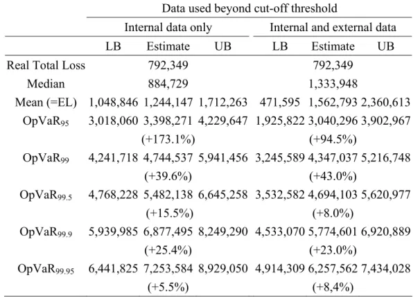
Table 9: Comparison of distributions obtained with or without external data for Cell (1,2)

Data used beyond cut-off threshold

Internal data only Internal and external data

LB Estimate UB LB Estimate UB

Real Total Loss 792,349 792,349

Median 884,729 1,333,948 Mean (=EL) 1,048,846 1,244,147 1,712,263 471,595 1,562,793 2,360,613 OpVaR95 3,018,060 3,398,271 (+173.1%) 4,229,647 1,925,822 3,040,296 (+94.5%) 3,902,967 OpVaR99 4,241,718 4,744,537 (+39.6%) 5,941,456 3,245,589 4,347,037 (+43.0%) 5,216,748 OpVaR99.5 4,768,228 5,482,138 (+15.5%) 6,645,258 3,532,582 4,694,103 (+8.0%) 5,620,977 OpVaR99.9 5,939,985 6,877,495 (+25.4%) 8,249,290 4,533,070 5,774,601 (+23.0%) 6,920,889 OpVaR99.95 6,441,825 7,253,584 (+5.5%) 8,929,050 4,914,309 6,257,562 (+8,4%) 7,434,028

This table presents estimates and the lower and upper bounds of 90% confidence intervals of the OpVaR for the Cell (1,2). The fitted distributions are a Negative Binomial (660, 0.476) for the frequency and the severity distribution is the combination of a Weibull (4,42, 0.094) for “ordinary” losses (from the collection threshold up to the cut-off threshold U = 537), a GPD (994; 1.412) for “large” losses (from U = 537 upwards). When including external data, the extreme threshold is 21,170 and a lognormal (12.37, 1.58) is used for “external” losses (above E = 21,170). Percentage increases with respect to the previous cell are shown between parentheses. To compute the confidence intervals, a bootstrap technique is applied: the severity distribution is fitted on a random sub-sample whose size is 90% of the original sample. The frequency distribution is a Negative Binomial (654, 0.459) for all iterations. The procedure is repeated 250 times.

Table 10: Operational RAROC

RAROCO Business line Default AMA Corrected AMA

Asset management 3.73% - Retail banking 3.13% -

TOTAL 3.48% 6.89%

In this table, the RAROCO figure represents the value of the operational risk adjusted return on

capital defined as , ) ( ) ( ) ( ) ( i Capital Economic i EL i GI i RAROCO op op op −

= when the revenues corresponding to

operational risk (GIop) are set equal to the gross operating margin of the business line (14% in our case). “Default AMA” corresponds to the default dependence assumption of Basel II (aggregation of capital charges) while “Corrected AMA” takes observed dependence into account.

Table 11: Impact of managerial actions on regulatory capital

Dashboards Audit Tracking

(1,1) (1,2) (2,1) (2,2) (1,1) (1,2) (2,1) (2,2) Frequency x 15 15 15 12 - 12 - 12

Severity y - - - - - 5 - 5

Expected Loss 13.0 10.7 12.7 18.6 - 12.4 - 23.5 Unexpected Loss 8.4 8.6 2.3 1.6 - 10.6 - 13.1 Reg. Capital (by cell) 8.3 8.5 1.9 0.6 - 10.4 - 11.7 Reg. Capital (by BL) 8.4 1.1 5.2 5.3

Reg. Capital (total) 4.7 5.8

This table reports the changes in (input) frequency and severity parameters and (output) loss and capital measures consecutive to a 15% reduction in the total expected loss. All elements of this table are expressed as percentage reductions.

Table 12: Impact of actions on profitability

Default AMA Dashboards Audit tracking Business Line RAROC A.C. RAROC A.C. RAROC A.C. Asset Mgmt 3.73% - 7.30% 1.48% 10.31% 2.28% Retail Banking 3.13% - 6.78% 0.36% 9.34% 0.59% TOTAL 3.48% - 7.08% 0.61% 9.95% 0.98%

In this table, the RAROCO figure represents the value of the operational risk adjusted return on

capital defined as , ) ( ) ( ) ( ) ( i Capital Economic i EL i GI i RAROCO op op op −

= when the Expected Loss (EL) is set equal

to 14% of the Gross Income (GI) corresponding the operational risk. “A.C.” means “Acceptable Cost” and represents the percentage amount of gross income generated by the business line that is necessary to reach a RAROC threshold of 18%.