A Google-inspired error-correcting graph matching algorithm

Titre:

Title

: A Google-inspired error-correcting graph matching algorithm

Auteurs:

Authors

: Segla Kpodjedo, Philippe Galinier et Giuliano Antoniol

Date: 2008

Type:

Référence:

Citation

:

Kpodjedo, S., Galinier, P. & Antoniol, G. (2008). A Google-inspired error-correcting graph matching algorithm (Rapport technique n° EPM-RT-2008-06).

Document en libre accès dans PolyPublie

Open Access document in PolyPublie URL de PolyPublie:

PolyPublie URL: https://publications.polymtl.ca/3166/

Version: Version officielle de l'éditeur / Published version_{Non révisé par les pairs / Unrefereed} Conditions d’utilisation:

Terms of Use: Tous droits réservés / All rights reserved

Document publié chez l’éditeur officiel

Document issued by the official publisher Maison d’édition:

Publisher: Les Éditions de l’École Polytechnique URL officiel:

Official URL: https://publications.polymtl.ca/3166/ Mention légale:

Legal notice: Tous droits réservés / All rights reserved

Ce fichier a été téléchargé à partir de PolyPublie, le dépôt institutionnel de Polytechnique Montréal

This file has been downloaded from PolyPublie, the institutional repository of Polytechnique Montréal

EPM–RT–2008-06

A GOOGLE-INSPIRED ERROR-CORRECTING GRAPH

MATCHING ALGORITHM

Segla Kpodjedo, Philippe Galinier, Giuliano Antoniol

Département de Génie informatique et génie logiciel

École Polytechnique de Montréal

EMP-RT-2008-06

A Google-inspired

error-correcting

graph matching algorithm

Segla Kpodjedo, Philippe Galinier,

Giuliano Antoniol

Département de génie informatique et génie logiciel

École Polytechnique de Montréal

A Google-inspired

error-correcting graph matching algorithm

Department of G´enie Informatique ´Ecole Polytechnique de Montr´eal — Canada

Abstract. Graphs and graph algorithms are applied in many different areas

in-cluding civil engineering, telecommunications, bio-informatics and software en-gineering. While exact graph matching is grounded on a consolidated theory and has well known results, approximate graph matching is still an open research subject.

This paper presents an error tolerant approximated graph matching algorithm based on tabu search using the Google-like PageRank algorithm. We report pre-liminary results obtained on 2 graph data benchmarks. The f rst one is the TC-15 database [14], a graph data base at the University of Naples, Italy. These graphs are limited to exact matching. The second one is a novel data set of large graphs generated by randomly mutating TC-15 graphs in order to evaluate the perfor-mance of our algorithm. Such a mutation approach allows us to gain insight not only about time but also about matching accuracy.

1 Introduction

Graph representations are well suited to modeling all kinds of real life objects or prob-lems. When one represents two given objects or problems as graphs, one legitimate question is to determine how similar (quantitatively and qualitatively) those two objects are. Do they share common parts and if so, to what extent and at what level of detail? Given two graphs, an intuitive way to answer these questions is to match, with respect to some constraints, the nodes and edges of the f rst graph to the nodes and edges of the second graph. In many areas, the generated or observed graphs are subject to all kinds of deformations or modif cations. Exact matching, which requires a strict cor-respondence among the two objects being matched or their subparts, often fails then to provide exploitable results. In this paper, we focus on approximate graph matching since real-life applications often fall into this category. Applications in different areas such as bioinformatics [8, 15], document processing [9] and video analysis [20] among others can be modeled as error tolerant graph matching problems.

Brief y, approximate graph matching algorithms allow matching two nodes that vio-late constraints such as the edge-preservation constraint - exact correspondence of edges - or any other characteristic such as node/edge labels, weights etc. Instead, a penalty is assigned to those constraint violations, depending on the specif c problem and desired results. In most cases, the best matching is considered to be the one that minimizes the

overall penalty cost. The problem is known to be NP-hard, and optimal algorithms suf-fer from prohibitive computation times on medium and large graphs. In this paper, we propose a tabu algorithm to address the approximate graph matching problem. Given penalty costs, our algorithm will try to f nd the optimal matching between two graphs. A similarity measure between two nodes of two different graphs can be def ned by ”how closely” those nodes are likely to match in the optimal matching. In graph matching, similarity measures prevent random matching by providing the probability of any given match. Our local search procedure uses a similarity measure combining local informa-tion on nodes, such as the number of edges (incoming and outgoing), with “global” information on nodes provided by what we call “structural metrics” computed via the Google-inspired PageRank algorithm [3]. PageRank [3], one of the main components behind the f rst versions of Google, basically measures the relative importance of each element of a hyperlinked set and assigns it a numerical weighting. In essence, the more references (incoming arcs) an element (vertex) gets from other elements (preferably important), the more importance it deserves. PageRank is linked to random walks on Markov chains. Its main advantage is its outstanding eff ciency in terms of computa-tion speed on sparse matrices, which is very convenient as real-world graphs are often sparse.

Furthermore, the literature on error-correcting graph matching benchmarks is very limited; to overcome this we propose a mutation algorithm to generate a mutated version of a given graph. We def ne as a mutation path, the set of edit operations applied to the original graph to obtain the mutated version. The computed cost of this mutation path from a graph to its mutated offspring provides us with an expected cost which is useful to evaluate the performances of approximate graph matching algorithms.

In this paper, we formalize the graph matching problem as an Error-Correcting Graph Matching (ECGM) problem [4]; then we introduce a mutation mechanism to produce approximate graph matching benchmarks and propose an enhanced tabu search algorithm for ECGMs.

The rest of the paper is organized as follows. Section 2 introduces the background notions of this paper. Then, the section 3 brief y reviews some of the most important related works. The fourth section gives more insights about our algorithm. Section 5 presents the case studies and the results of our algorithm. The paper concludes with discussion and indications of future work.

2 Background Notions

In this section, we present the def nitions for an error correcting graph matching prob-lem as formulated in [4] and the basic principles of the PageRank algorithm.

2.1 Problem Statement

The following def nitions, mostly adapted from [4], contextualize the error correcting graph matching in a theoretical framework.

Def nition 1. Given two f nite alphabets of symbols, PV and PE, we def ne a

vertices; LV : V → P_V is the node labeling function; LE : V × V →P_Eis the

edge labeling function.

To simplify problem formulation it is assumed graphs are fully connected; the spe-cial label null is assigned to non-edges. The set of edges E is then implicitly given by considering only edges with a label different from null. In the following, we will refer to non-edges as edges assigned the null label and effective edges as edges assigned with a label other than null

Def nition 2. Let g1 = (V1, LV1, LE1)and g2 = (V2, LV2, LE2)be two graphs.

An error-correcting graph matching (ECGM) from g1 to g2 is a bijective function

f : ˆV1→ ˆV2where ˆV1⊆ V1, ˆV2⊆ V2. We say x ∈ ˆV1is substituted by node y ∈ ˆV2if

f(x) = y. Furthermore, any node from V1− ˆV1is deleted from g1, and any node from

V2− ˆV2is inserted in g2under f. We will use ˆg1and ˆg2to denote the subgraphs of g1

and g2that are induced by the sets ˆV1and ˆV2, respectively.

The mapping f indirectly implies edit operations on the edges of g1 and g2. If

f(x1) = x2and f(y1) = y2, then the edge (x1, y1)is substituted by edge (x2, y2). If

a node x1 is deleted from g1, then any edge incident to x1 is deleted, too. Obviously,

any ECGM can be understood as a set of edit operations (substitutions, deletions, and insertions of both nodes and edges) that transform a given graph g1into another graph

g2).

Def nition 3. The cost of an ECGM f : ˆV1→ ˆV2from a graph g1= (V1, LV1, LE1)

to a graph g2= (V2, LV2, LE2)is given by c(f ) = X x₁∈ ˆV₁ cns(LV1(x1), LV2(f (x1))) + X x₁∈V1− ˆV1 cnd(LV1(x1)) + X x2∈V2− ˆV2 cni(LV2(x2)) + X (x1,y1)∈ ˆE1 ces(LE1((x1, y1)), LE2((f (x1), f (y1)))) + X (x₁,y₁)∈E₁− ˆE₁ ced(LE1((x1, y1))) + X (x₂,y₂)∈E₂− ˆE₂ cei(LE2((x2, y2))) (1) where cns(LV1(x1), LV2(f (x1)))is the cost of substituting a node x1∈ ˆV1by the

label of f(x1) ∈ ˆV2; cnd(LV1(x1))is the cost of deleting a node x1 ∈ V1− ˆV1from

g1; cni(LV2(x2))is the cost of inserting a node x2∈ V2− ˆV2in g2; ces(LE1((x1, y1)),

LE2((f (x1), f (y1)))) is the cost of substituting an edge e = (x, y) ∈ ˆE1 by e′ =

(f (x), f (y)) ∈ ˆE2; ced(LE1((x1, y1)))is the cost of deleting an edge e ∈ E1− ˆE1

from g1and cei(LE2((x2, y2)))is the cost of inserting an edge e ∈ E2− ˆE2in g2.

The shorthand notations E1, ˆE1, E2, ˆE2are used for V1×V1, ˆV1× ˆV1, V2×V2, ˆV1×

ˆ

V1, respectively. Formula 1 present our cost function which is actually the sum of the

cost of edit operations. As presented, those costs are def ned using nodes/edges labels. For instance, Ces(l1, l2)is the cost of substituing an edge labeled l1by an edge labeled

l2, while Ced(l1)is the cost for deletingan edge labeled l1from the f rst graph .

For simplif cation purposes, one can use single values for specif c edit operations such as a constant value for all node addition operations. Nevertheless, our approach can accomodate a higher level of detail if required. The term “edge substitution” in

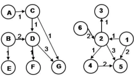
Fig. 1. Examples of graphs to be matched

the previous def nition is related to different operations one might want to distinguish. Thus, we identify

– cesiIdentical edge label substitution

– cessStructural error : edge substitution involving an effective edge and a non-edge

– cesl Label error : edge substitution involving two effective edges with different

labels

Let cnsbe the cost for substituing any node assigned a label l1by another assigned l2,

with l1 6= l2; cndthe cost of deleting any node from g1; cnithe cost of inserting any

node in g1; cedthe cost of deleting any effective edge from g1; ceithe cost of inserting

any effective edge in g2. Any ECGM cost function could then be represented by the

octuple (cns, cnd, cni, ced, cei, cesi, cess, cesl). The cost of an identical edge label

sub-stitution should be 0. Furthermore, if symmetry is wanted or irrelevant, one can use the same value for deletions/insertions. From the initial octuple, one can keep the quintu-ple (cns, cno, ceo, cess, cesl) to def ne any ECGM cost function; cno(respectively ceo)

being the cost of adding/removing any node (respectively any edge). For instance, (cns,

cno, ceo, cess, cesl) = (∞, 1, 0, ∞, ∞) corresponds to the maximum common subgraph

problem. The values of those costs could be related to the probability of occurrence of the associated distortions. Therefore, one may want the cost of a structural error to be inferior to that of a label error, if changing the type of relation between two nodes is less likely than simply dropping / losing that relation.

Example: Given the cost function (cns, cno, ceo, cess, cesl) = (0, 2, 1, 12, 7) and the

two labeled graphs on Figure 1, one may be interested in f nding the optimal matching. Notice here that we assumed a cost of modifying an edge with label modif cation (i.e., Cesl) substantially higher than the cost of inserting/deleting a node (i.e., Cno).

2.2 PageRank

PageRank allow us to assign a metric representative of global structure for each vertex of a given graph. This global metric is the outcome of a Random Walk (RW) on the graph which is a probabilistic model used to compute the probability uv(t)of being

lo-cated in a given vertex v at time t. A random walker on a graph proceeds iteratively by moving from a vertex v1to a vertex v2following the arc (v1, v2)or by jumping directly

(with respect to a f xed low probability) to v2. The probability distribution on all the

ver-tices of a given graph G = (V,E) is represented by a vector u(t) = [u1(t); ...; u|V |(t)].

The vector of probabilities is updated at each step and is proven to converge to a stable solution. Further details can be found in [19] which proposes a very eff cient algorithm to compute u(t). The point here is the use of an eff cient algorithm providing a global metric for each vertex of a graph. For instance, given a jump probability of 0.1, we ob-tain u(t) = [0.014; 0.014; 0.14; 0.16; 0.057; 0.046; 0.175], for the f rst graph on Figure 1. In that graph, the nodes G, D, C have the highest values.

3 Related Works

Conte et al. [10] in their review of graph matching algorithms classify the existing methods into three main categories: techniques based on tree search, techniques based on continuous optimization, spectral methods. This classif cation is completed by “other techniques” such as genetic algorithms etc.

In techniques based on tree search, the search - with backtracking - is directed by the cost of the partial solution obtained so far and various heuristics are used to prune paths which are estimated as unfruitful or, on the contrary, prioritize the most promis-ing paths. The range and power of prediction of those proposed heuristics [1] are es-sential for reasonable computation times. Some authors investigated approaches aimed at redef ning or simplifying the graph matching problem. For example, decomposition techniques are presented in [13], while transformation models are the focus in [11].

Some tree-search based techniques lead to the def nition of optimal algorithms [12]; however, the major drawback of this category of techniques is the often prohibitive computation times required when the size of the graphs increases.

The literature is rich in fast and eff cient, if not optimal, algorithms designed to resolve continuous optimization problems. This explains the popularity of this family of techniques, even if it means, as in this case, casting an inherently discrete problem into a continuous, non linear problem, solving it with a continuous optimization technique, and eventually converting the - often non-optimal - obtained solution back into the initial discrete problem. Different methods are available from “simple” probabilistic relaxation framework [16] to the def nition of a Bayesian graph edit distance [18], or reformulation as Weighted Graph Matching [2, 26].

Considering two isomorphic graphs, their node-to-node adjacency matrices will have the same eigenvalues and eigenvectors. The converse may not be true and infor-mation gained may be only structural, thus lacking all kinds of other useful inforinfor-mation about a graph, but this is still an interesting starting point for a graph matching prob-lem and, among some others, Umeyama [24] pioneered the above idea. Of course, as far as approximate matching is concerned, the obtained results will gain in accuracy as the considered graphs are nearly isomorphic. In such cases, spectral techniques [6] ro-bust to the distortions can be successfully applied. In the literature, spectral features are combined with other methods like continuous optimization techniques [17], clustering techniques [7, 6, 21] or are simply used to guide a greedy search procedure [22].

Closer to the algorithm presented in this work is [21], in which random [16]walks provide topological features further used with clustering techniques.

Among the ”other techniques” previously mentioned, we can underline the use of meta-heuristics such as genetic algorithms [5, 23], simulated annealing [13] and tabu search [25].

Overall, our review of the literature supports the opinion that most algorithms and results are application-driven; furthermore ECGM benchmarks are not publicly avail-able. This prevents simple and clear comparisons between the different approaches and algorithms. Finally, most often, the graphs considered are usually quite small (less than 100 nodes).

4 The Algorithm

In the following, we consider an ECGM problem instance def ned by a triple (G1, G2, C)

with G1being the f rst graph, G2the second graph and C the cost parameters as def ned

in Section II. The choice of the cost parameters steers the type of matching found. 4.1 Overview of the tabu search

Our algorithm is a Tabu Search (TS) algorithm guided by global information on the nodes from the PageRank algorithm and local node features such as the number of edges. In the following paragraph, we summarize the key ideas behind a tabu algorithm. Given a function f (cost function) to be minimized (or maximized) over some set S(the Search Space), a local search technique starts from some initial feasible point (solution) in the search space and proceeds iteratively (moves) from one point in S

to another (a neighbor) until some termination criterion is met. There is no guarantee of obtaining an optimal solution as the search may get trapped in local optima, but some techniques are proven very helpful in avoiding local optima and f nding good solutions. For instance, to prevent cycles in the search, TS introduces one or several tabu lists (short term memory) used to exclude moves which would tend to make the search process go back to a previously visited solution. Other lists for intermediate and long-term memory may be used to intensify the search in a promising area of the search space or diversify the search to previously unexplored areas.

Given two graphs G1= (V1, LV1, LE1)and G2= (V2, LV2, LE2), we def ne as a

match any pair (n1i, n2j) ∈(V1× V2). We def ne a solution S as a subset of V1× V2:

S⊂ V1× V2and (a, b), (c, d) ∈ S, (a, b) 6= (c, d) ⇒ a 6= c and b 6= d.

Since we are interested in one-to-one matching, a legal solution excludes multiple matches, i.e. if S contains the pair (n1i, n2j), n1iand n2jcannot be in any other match

of S. The search space is the set of all legal solutions. Given a current solution, the only moves permitted are match insertion + and match removal - i.e. one can only insert a match of nodes missing from any match of the current solution. Considering, as described in Section II, that each solution S def nes ˆV1, the set of matched nodes of

V1and ˆV2, the set of matched nodes of V2, the neighborhood N(S) of a solution S is

def ned by the following moves S

ր+(n1i, n2j) ∈ ((V1− ˆV1) × (V2− ˆV2)) ց

or

ց-(n1, n2) ∈ S ր

We use two tabu lists in our algorithm : one for a match just inserted (T ABUOU T)

and one for a match just deleted ( T ABUIN ). The T ABUOU T list prohibits for a

certain period the removal of a just inserted match, while the T ABUIN list prevents a

just deleted match to be reinserted before a certain number of moves. 4.2 Similarity Measure and moves

Given a solution S and a move m: S → S′_{, we def ne delta cost δ}

m= f (S′) − f (S)as

the differential of cost brought by the move m.

Generally, in a local search algorithm, given a solution S, the choice of a move m is essentially guided by its δm. However, in our problem, a choice based solely on this

local information, on the search space, may lead to poor performance, both in terms of computation and matching accuracy.

At the beginning of the search, when the f rst matching is chosen, there is typically a very large number of possible choices with the same best possible performance. There-fore, erroneous choices are very likely to occur at the beginning of the search. and they may compromise the f nal solution. Our empirical results conf rm that assumption, as very poor results were obtained.

To make a search eff cient, our idea is to use available information for each of the two graphs. Local features of a node, such as its degree, are natural candidates for the implementation of this idea. In our algorithm, local information of a vertex v is a feature vector loc(v) = (vin, vout)with vinbeing the number of incoming edges and vout the

number of outgoing edges. This is a f rst valuable information one can use to weight the match of two nodes v1 ∈ V1 and v2 ∈ V2. Given a node n1 of a graph G1and a

node n2of a graph G2, their respective number of incoming edges ei1, ei2and number

of outgoing edges eo1, eo2,the local similarity metric l(n1,n2)is computed as follows

l(n1,n2) = 1 −

p(ei,1− ei,2)2+ (eo,1− eo,2)2

max(qe2_i,1+ eo,12, q

e2_i,2+ e2 o,2)

∈ [0, 1]

We then resort to global information about a node and select a very fast algorithm : the PageRank algorithm [19]. Note that we generate the metrics on nodes without taking into account the edge labels. Thus, the obtained metrics are purely structural. The nodes are sorted in a descending order of that metric. Given a node n1of a graph

G1 and a node n2 of a graph G2, their respective ranks rank(n1) and rank(n2), the

global similarity metric g(n1,n2)is computed as follows

g(n1,n2) = 1 −     rank(n1) |V1| − rank(n2) |V2|     ∈ [0, 1]

Note that the global similarity metric of a given node may change dramatically due to the insertion or removal of a single incoming edge. The local similarity metric will be particularly useful in those extreme situations. For each possible match m = (n1i, n2j),

with n1i ∈ V1 and n2j ∈ V2, we compute as follows a weight wij designed to be a

measure of the likelihood of this match. In order to combine the two metrics (local and global), we weight them with coeff cients. We assume that the higher the degree of a

node, the fewer are its possible matches in the other graph; this makes the similarity measure more trustable as high values of similarity will be observed for a restricted number of matches. Similarly, the higher the rank of a node, the more relevant its global similarity values; coeff cients are def ned as follows:

gcoef f(n1,n2) = 1 −1₂ × (rank(n_|V 1)

1| +

rank(n2)

|V2| ) ∈ [0, 1] lcoef f(n1,n2) = 1₂× (degdeg(nmax(V1)1)+

deg(n1)

degmax(V1)) ∈ [0, 1]

degmax(V1)(resp. degmax(V2)) is the highest degree of a node found in V1(resp. V2).

gcoef f(n1,n2)and lcoef f(n1,n2)are the respective weights of the global and local

sim-ilarity measures in the computation of the f nal simsim-ilarity measure: wij = 1 −

lcoef f(n1n2)×l(n1n2)+gcoef f(n1n2)×g(n1,n2)

2 ∈ [0, 1]

Given a move mv = operation((n1, n2)), with n1 ∈ V1 and n2 ∈ V2 and its

cost δm, we recompute the delta brought by a movement as follows. If mvis a match

insertion, we grant mva bonus to encourage the insertion of the match (n1, n2):

δmv = δm− (wij× M AXincentives)

Else, i.e. mv is a match removal, we grant mv a malus to discourage the removal of

(n1, n2).

δmv = δm+ (wij× M AXincentives)

M AXincentivesrepresents the maximum of incentives given to a match. The weights

wijare def nitively computed at the initialization of the algorithm. They are used to bias

the δmof the moves.

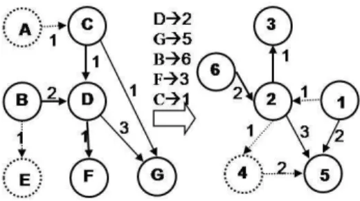
Application to the example Given the cost function (cns, cno ceo, cess, cesl) =

(0, 2, 1, 12, 7), we want to f nd the best matching for the two graphs in Figure 1. Initially, we have an empty solution, no matching, whose cost is 40. In this empty solution, we have to pay for all the nodes and edges deleted (7*2 + 7*1 = 21), and At Step 0, in our example, all moves have the same delta cost δm= cns− (cni+ cnd) = −4. When we

apply the bonus of the computed similarity metrics, we obtain, with MAXincentives=

4, Table 4.2. (D,2) having the least cost is selected, and the δm are recomputed, if

required. In this way, our similarity measure guides our local search. The process is iterated and, for that example, the best solution is S = {(D,2) (G,5) (C,1) (F,3) (B,6)} with cost(S) = 17 as shown in Figure 2.

5 Case Studies

To the best of our knowledge, only a few works have addressed the ECGM problem and no reference or standard database of large graphs for such problem exists. The ex-isting literature does not report or mention benchmarks for ECGM algorithms. Most of the past contributions are application-driven and results on presented algorithms are

1 2 3 4 5 6 A -4 -4 -4 -4 -4 -5 B -5 -5 -4 -4 -4 -4 C -5 -6 -5 -5 -5 -4 D -4-7 -5 -5 -5 -4 E -4 -5 -5 -5 -5 -4 F -4 -4 -5 -5 -4 -4 G -4 -5 -5 -5 -6 -4

Table 1. Modif ed δmof the moves at step 0

Fig. 2. Example of approximated graph matching.

reported on their own specif c datasets. Moreover, the graphs are rarely publicly avail-able. To overcome such a limitation we apply a twofold strategy. First, given that no specif c dataset was found, we f rst applied our algorithm to a subsets of graph taken from the TC-15 Graph Database [14]. Then we applied a mutation strategy outlined in the following mutation subsection to generate a set of graph pairs with known distor-tion. In essence, by deleting, adding or modifying graph elements we generate graph pairs where a near optimal matching is known.

5.1 The Graph Database

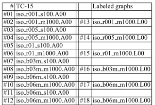
The Graph Database of [14], also called TC-15 Database, is a large benchmark for ex-act graph matching problems such as graph isomorphism, subgraph isomorphism and maximum common subgraph. TC-15 contains three different kind of graphs: randomly connected, bound valence and mesh. We selected the f rst two categories as most rel-evant for our problem. In these two categories (i.e., randomly connected and bound valence graphs) TC-15 contains several subcategories. For each available subcategory we selected a large (about 1000 nodes) and a medium (about 100 nodes) graph. In par-ticular we selected the categories of randomly connected graphs (iso r***) and mod-if ed bound valence graphs (iso b**m). For each of their subcategories, we chose the f rst graphs (.A00) of order 100 and 1000. Table 2 presents our selection. In essence, we selected in TC-15 the subsets of large graphs likely to represent most encountered matching problems.

# TC-15 Labeled graphs #01 iso r001 s100.A00

#02 iso r001 m1000.A00 #13 iso r001 m1000.L00 #03 iso r005 s100.A00

#04 iso r005 m1000.A00 #14 iso r005 m1000.L00 #05 iso r01 s100.A00

#06 iso r01 m1000.A00 #15 iso r01 m1000.L00 #07 iso b03m s100.A00

#08 iso b03m m1000.A00 #16 iso b03m m1000.L00 #09 iso b06m s100.A00

#10 iso b06m m1000.A00 #17 iso b06m m1000.L00 #11 iso b06m s100.A00

#12 iso b06m m1000.A00 #18 iso b06m m1000.L00 Table 2. Selected graphs from TC-15 and labeled graphs.

It is worth mentioning that all these graphs are unlabeled, while our algorithm is able to deal with labeled graphs. We annotated, with labels, edges of TC-15 graphs to obtain labeled graphs. Labels were drawn randomly from uniform distribution with labels in an alphabet of 4 letters LE = {1, 2, 3, 4}. The graphs obtained are presented

in Table 2. 5.2 Mutation

To obtain a set of ECGM specif c problems with controlled distortion we applied mu-tation to transform a given graph G1into another graph G2.

The advantage is substantial since we keep track of the edit operations our mutation algorithm performs; these operations correspond to a path from G1to G2. That means,

knowing which node has been deleted, inserted, substituted from G1to G2, we have,

de facto, for our two graphs a very good known matching which we call MM(G1, G2)

for Mutation Matching with a known Exact Mutation Matching Cost (EMMC). In essence, since G2is the result of a mutation algorithm we know the exact

trans-formation applied and thus we know a nearly ideal matching and the expected cost against which results obtained by ECGM algorithms can be compared. EMMC is then a very good upper bound for our matching problem, especially when the original graph is lowly distorted. For highly distorted graph pairs where the original graph structure is severely disrupted, we cannot guarantee that there does not exist a matching cost lower than EMMC. This is not a surprise since as we introduce more and more edit opera-tions, it is more likely that good alternatives to MM(G1, G2)can be found. Overall,

the lower the distortion and the noise introduced, the closer the EMMC value will be to the optimal cost. A theoretical study of relation between distributions of edit operations and relations with upper and lower bounds are beyond the scope of this paper and will be the subject of future works.

In this work we consider simple distortions such as : node/edge deletions, node/edge insertions and node/edge substitutions. The edit operations were assigned probabilities of occurrence and applied based on algorithms described below.

The mutation algorithm has a two steps beginning with what we called node noise, followed by edge noise. Note that all the edges inserted or modif ed are assigned labels with respect to the edge label distribution in G1. Our mutation algorithm takes three

parameters, pnd(probability of node deletion), pna (probability of node addition) and

pedge(noise on edges). First it performs a shuff e of nodes with labels randomly

as-signed, then nodes are deleted, and in the subsequent steps, nodes are added before we f nally apply noise on edges.

The node noise is applied using pnd and pna. More precisely, the node deletion

algorithm parses all the nodes of the graphs and decides, according to pnd, to delete

or not the considered node. Similarly, the node addition algorithm parses all the nodes of the graphs and decides, according to pna, to add or not a new node. When a node

is deleted, its edges are deleted as well. After all nodes have been added, edges are added in an attempt to preserve the graph density. Given the number of new nodes nodesnewand the density doof the original graph, we compute the number edgesnew

of edges which should be linked to the set of new nodes edgesnew= nodesnew× do=

insertiontrials. For insertiontrialsiterations, we randomly choose two nodes of the

mutated graph and effectively insert an edge if at least one of the chosen nodes is a new one. When an edge is inserted, we assign it a label with respect to the edge label distribution in the original graph.

Once the node deletion and addition phases are completed, we apply the edge noise algorithm with the parameter pedge which represents the probability of modifying an

effective edge. An edge substitution can result in a simple edge label substitution or an edge deletion. After the effective edge substitution stops, we proceed to edge insertions. In order to preserve the overall density of the graph, we recompute the probability to insert a new edge as follows : pei =

deletededges

mnull , with deletededges the number of deleted effective edges in the previous step and mnull the number of non-edges (i.e.,

null edges) in the mutated graph. For each non-edge, an effective edge is inserted or not according to pei. Whenever we modify/insert/delete an edge we do it by using a biased

wheel where the weight of each label is its percentage of occurences in the original graph.

Applying the above described graph mutation strategy, we generate a mutated graph G2 from G1 with a known set of applied transformation. The EMMC value is then

computed by applying Formula 1 (Def nition 3). 5.3 ECGM results

We apply our mutation algorithm to the selected graphs in the TC-15 dataset with dif-ferent parameters. Considering the triple (pnd, pna, pedges) it is possible to generate

graph tailored for different kinds of graph matching problems. 1. (0, 0, 0) : graph isomorphism

2. (0, pna,0): subgraph isomorphism

3. (pnd, pna,0): maximum common subgraph

4. (pnd, pna, pedges): ECGM

Provided that the values of the parameters are kept small, the f rst three categories of mutation conf gurations can be used to obtain good approximations for optima values in corresponding exact matching problems while the last category is specif c to ECGMs.

In this f rst set of experiments, we empirically selected the following weights for our cost function (cns, cno, ceo, cess, cesl) = (0, 2, 1, 12, 7). We applied our tabu

algo-rithm to each of the pairs (G, Gmutated)with different noise parameters; we empirically

f xed the length of the tabu lists as follows : T ABUIN(10)and T ABUOU T(20); the

value MAXincentives is set to the highest edit cost : cesl = 12; each experiment was

replicated ten times. Results collected and summarized in Tables 3 and 4.

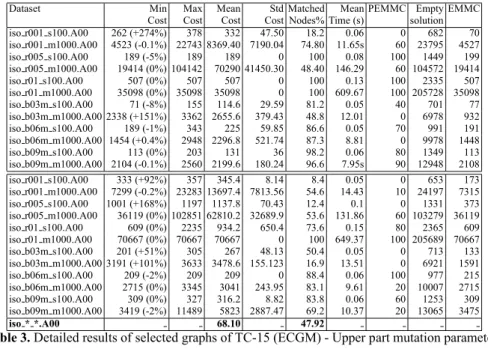
Tables are organized as follows. The Mutation column shows the three probability values, as percentages, applied to mutate the graph identif ed in column one. Thus the sequence “5 5 1” mean 5 % probability of deleting or adding a node and 1 % probability of adding noise to one edge. For each mutated graph, ECGM algorithm was run ten times and data was collected; columns min, max and mean cost report respectively the minimum, maximum and average cost in the ten trials. We indicate how far the best result of the algorithm is from the EMMC in the brackets of column min Cost, reporting this distance in terms of percentage. To obtain evidence of the dispersion of the matching cost, we computed the cost’s standard deviation as reported in the f fth column Std Cost. The Matched nodes column is one of the key f gures to judge the algorithm performance in that it represents the percentage of correctly matched nodes with respect to the MM(G1, G2) transformation. The average time in the ten runs

required to obtain a match is shown in column “Mean Time”.

ECGM algorithms f nd optimal or near optimal solutions by minimizing some cost functions. Column PEMMC (percentage of EMMC) reports the percentage of times in the ten trials in which the exact value EMMC was attained. A naive approach would be to discard all nodes from the f rst graph and add nodes and edges to an empty graph so that the second graph is obtained; the cost of such a solution is reported in the penulti-mate column labeled empty solution. Finally the last column contains the EMMC value. Results reported in the tables refer to different possible conf gurations: unlabeled versus labeled graphs. We report results for mutated unlabeled graphs in Table 3 and mutated labeled graphs in Table 4.

We report the percentage of nodes matched to their distorted versions (column Matched Nodes) and the number of times we reached the upper bound cost (PEMMC) as relevant accuracy indices.

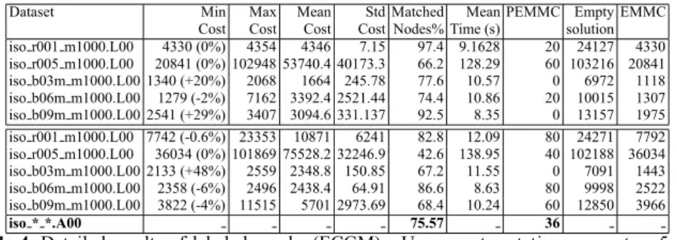
On unlabeled graphs, we have an average of about 68 % of correctly matched nodes (see Table 3) attaining about 48 % of the time the value of EMMC. Labels on edges help the algorithm as shown in Table 4, indeed, the authors believe that a value of 76 % of correct matching with an average PEMMC of 36 % can be considered very good. In fact, more than two thirds of the distorted nodes are correctly retrieved. Also, those results are just an average of ten trials and a detailed analysis of Tables 3 and 4 showed that within the ten runs, our algorithm failed to reach the upper bound for only 7 of the 24 ECGM unlabeled datasets and 3 of the 10 ECGM labeled datasets. We be-lieve that although the average PEMMC is not very high, we can f nd good perspectives in the high percentage of ”correctly” matched nodes. This proves we generally hit the good search areas despite the empiric values of our cost function. Notice that differ-ent penalty costs may provide better or worse results for this performance indice. As shown in Table 3, some graphs like iso r01 s100.A00 mutated with parameters (5 5 1) or iso b03m m1000.A00 mutated with (10 10 2) gave very poor results. This can be

explained by considering the graph density. We have found that given a graph with low density, adding and deleting edges can easily result in a drastic and deep structure change. For instance, graphs low both in density and in order can mutate in various sets of disconnected graphs with various f oating islands. These are isolated mini-graphs which are very hard to map back into the original structure. Computation time is gen-erally low and acceptable for applications where the algorithm is run off-line, which is what we are considering, .

Dataset Min Max Mean Std Matched Mean PEMMC Empty EMMC Cost Cost Cost Cost Nodes% Time (s) solution iso r001 s100.A00 262 (+274%) 378 332 47.50 18.2 0.06 0 682 70 iso r001 m1000.A00 4523 (-0.1%) 22743 8369.40 7190.04 74.80 11.65s 60 23795 4527 iso r005 s100.A00 189 (-5%) 189 189 0 100 0.08 100 1449 199 iso r005 m1000.A00 19414 (0%) 104142 70290 41450.30 48.40 146.29 60 104572 19414 iso r01 s100.A00 507 (0%) 507 507 0 100 0.13 100 2335 507 iso r01 m1000.A00 35098 (0%) 35098 35098 0 100 609.67 100 205728 35098 iso b03m s100.A00 71 (-8%) 155 114.6 29.59 81.2 0.05 40 701 77 iso b03m m1000.A00 2338 (+151%) 3362 2655.6 379.43 48.8 12.01 0 6978 932 iso b06m s100.A00 189 (-1%) 343 225 59.85 86.6 0.05 70 991 191 iso b06m m1000.A00 1454 (+0.4%) 2948 2296.8 521.74 87.3 8.81 0 9978 1448 iso b09m s100.A00 113 (0%) 203 131 36 98.2 0.06 80 1349 113 iso b09m m1000.A00 2104 (-0.1%) 2560 2199.6 180.24 96.6 7.95s 90 12948 2108 iso r001 s100.A00 333 (+92%) 357 345.4 8.14 8.4 0.05 0 653 173 iso r001 m1000.A00 7299 (-0.2%) 23283 13697.4 7813.56 54.6 14.43 10 24197 7315 iso r005 s100.A00 1001 (+168%) 1197 1137.8 70.43 12.4 0.1 0 1331 373 iso r005 m1000.A00 36119 (0%) 102851 62810.2 32689.9 53.6 131.86 60 103279 36119 iso r01 s100.A00 609 (0%) 2235 934.2 650.4 73.6 0.15 80 2365 609 iso r01 m1000.A00 70667 (0%) 70667 70667 0 100 649.37 100 205689 70667 iso b03m s100.A00 201 (+51%) 305 267 48.13 50.4 0.05 0 713 133 iso b03m m1000.A00 3191 (+101%) 3633 3478.6 155.123 16.9 13.51 0 6921 1591 iso b06m s100.A00 209 (-2%) 209 209 0 88.4 0.06 100 977 215 iso b06m m1000.A00 2715 (0%) 3345 3041 243.95 83.1 9.61 20 10007 2715 iso b09m s100.A00 309 (0%) 327 316.2 8.82 83.8 0.06 60 1253 309 iso b09m m1000.A00 3419 (-2%) 11489 5823 2887.47 69.2 10.37 20 13065 3475 iso * *.A00 68.10 47.92

Table 3. Detailed results of selected graphs of TC-15 (ECGM) - Upper part mutation parameters

5 5 1; lower part 10 10 2.

6 Conclusion

We have presented an algorithm inspired by Google PageRank to f nd optimal or near optimal solutions to the class of problems of approximate, error tolerant graph matching where it is acceptable to match two nodes that violate constraints such as the edge-preservation constraint or any other characteristic such as node/edge labels or weights.

Inspired by the work of previous authors [3, 4, 21] we represented the approxi-mate graph matching problem as an optimization problem modeled by cost matrices accounting for the cost of various edit operations (e.g., node insertion and deletion). Our algorithm relies on a tabu search; our search procedure combines local informa-tion on nodes (e.g., the number of incoming edges) with “global” informainforma-tion on nodes provided by “structural metrics” computed via the PageRank algorithm [3].

Dataset Min Max Mean Std Matched Mean PEMMC Empty EMMC Cost Cost Cost Cost Nodes% Time (s) solution iso r001 m1000.L00 4330 (0%) 4354 4346 7.15 97.4 9.1628 20 24127 4330 iso r005 m1000.L00 20841 (0%) 102948 53740.4 40173.3 66.2 128.29 60 103216 20841 iso b03m m1000.L00 1340 (+20%) 2068 1664 245.78 77.6 10.57 0 6972 1118 iso b06m m1000.L00 1279 (-2%) 7162 3392.4 2521.44 74.4 10.86 20 10015 1307 iso b09m m1000.L00 2541 (+29%) 3407 3094.6 331.137 92.5 8.35 0 13157 1975 iso r001 m1000.L00 7742 (-0.6%) 23353 10871 6241 82.8 12.09 80 24271 7792 iso r005 m1000.L00 36034 (0%) 101869 75528.2 32246.9 42.6 138.95 40 102188 36034 iso b03m m1000.L00 2133 (+48%) 2559 2348.8 150.85 67.2 11.55 0 7091 1443 iso b06m m1000.L00 2358 (-6%) 2496 2438.4 64.91 86.6 8.63 80 9998 2522 iso b09m m1000.L00 3822 (-4%) 11515 5701 2973.69 68.4 10.24 60 12850 3966 iso * *.A00 75.57 36

Table 4. Detailed results of labeled graphs (ECGM) - Upper part mutation parameters 5 5 1;

lower part 10 10 2

To quantify performance of our algorithm we selected a subset of medium and large graphs from the TC-15 benchmark, which is designed for exact graph matching prob-lems, and generated mutated graph versions with different level of distortions. These graphs are available for downloading at the SOftware Cost-effective Change and Evo-lution Research (SOCCER) laboratory1_.

We report accuracy and performance of our algorithm on the above mentioned set as well on the original TC-15 dataset. On an ECGM problem and labeled graphs, on average, we attain an average about 76 % of accurate node matching for graphs of about 1000 nodes. Computation time is in the order of a couple of minutes which we believe is acceptable for the off-line type of applications we foresee for our algorithm.

Future work will be devoted to assessing algorithm accuracy for larger graphs (e.g., 8,000 nodes and 80,000 edged). Also we believe it is important to better investigate more thoroughly the impact of different cost schema in the cost function as well as the inf uence of various kinds of distortions on algorithm performance.

References

1. M. Y. A. K. C. Wong and S. C. Chan. An algorithm for graph optimal monomorphism. IEEE

Trans. Syst. Man Cybern., 20:628–638, 1990.

2. H. A. Almohamad and S. O. Duffuaa. A linear programming approach for the weighted graph matching problem. IEEE Trans. Pattern Anal. Mach. Intell., 15(5):522–525, 1993. 3. S. Brin and L. Page. The anatomy of a large-scale hypertextual web search engine. Comput.

Netw. ISDN Syst., 30(1-7):107–117, 1998.

4. H. Bunke. On a relation between graph edit distance and maximum common subgraph.

Pattern Recogn. Lett., 18(9):689–694, 1997.

5. J. T. H. C. W. Liu, K. C. Fan and Y. K. Wang. Solving weighted graph matching problem by modif ed microgenetic algorithm. In IEEE Int. Conf. Syst. Man Cybern., pages 638–643, 1995.

6. T. Caelli and S. Kosinov. An eigenspace projection clustering method for inexact graph matching. IEEE Trans. Pattern Anal. Mach. Intell., 26(4):515–519, 2004.

7. M. Carcassoni and E. R. Hancock. Weighted graph-matching using modal clusters. In CAIP

’01: Proceedings of the 9th International Conference on Computer Analysis of Images and Patterns, pages 142–151, London, UK, 2001. Springer-Verlag.

8. Cheng, Saigo, and Baldi. Large-scale prediction of disulphide bridges using kernel meth-ods, two-dimensional recursive neural networks, and weighted graph matching. In Proteins:

Structure, Function, and Bioinformatics, volume 62, pages 617 – 629, 2006.

9. D. Conte, P. Foggia, , C. Sansone, and M. Vento. Graph matching applications in pattern recognition and image processing. In ICIP03, pages II: 21–24, 2003.

10. D. Conte, P. Foggia, C. Sansone, and M. Vento. Thirty years of graph matching in pattern recognition. International Journal of Pattern Recognition and Artif cial Intelligence, 18:265– 294, 2004.

11. L. P. Cordella, P. Foggia, C. Sansone, and M. Vento. An eff cient algorithm for the inexact matching of arg graphs using a contextual transformational model. In ICPR ’96: Proceedings

of the International Conference on Pattern Recognition (ICPR ’96) Volume III-Volume 7276,

pages 180–184, Washington, DC, USA, 1996. IEEE Computer Society.

12. A. C. M. Dumay, R. J. van der Geest, J. J. Gerbrands, E. Jansen, and J. H. C. Reiber. Consis-tent inexact graph matching applied to labeling coronary segments in arteriograms. In Proc.

Int. Conf. Pattern Recognition, Conf. C (1992), pages 439–442, 1992.

13. A. A. Eshera and K. S. Fu. A similarity measure between attributed relational graphs for image analysis. In Proc. 7th Int. Conf. Pattern Recognition, pages 75–77, 1984.

14. P. Foggia, C. Sansone, and M. Vento. A database of graphs for isomorphism and subgraph isomorphism benchmarking. In Proc.Third IAPR TC-15 Intl Workshop Graph-Based

Repre-sentations in Pattern Recognition, pages 176–187, 2001.

15. I. Jonassen. Eff cient discovery of conserved patterns using a pattern graph. 13(5):509–522, 1997.

16. J. Kittler and E. R. Hancock. Combining evidence in probabilistic relaxation. Int. J. of Patt.

Recogn. Artif. Intell, 3:29–51, 1989.

17. B. Luo and E. Hancock. Structural graph matching using the em algorithm and singular value decomposition. IEEE Trans. Pattern Anal. Mach. Intell., 23(10):1120–1136, 2001. 18. R. Myers, R. C. Wilson, and E. R. Hancock. Bayesian graph edit distance. IEEE Trans.

Pattern Anal. Mach. Intell., 22(6):628–635, 2000.

19. L. Page, S. Brin, R. Motwani, and T. Winograd. The pagerank citation ranking: Bringing order to the web. Technical report, Stanford Digital Library Technologies Project, 1998. 20. M. Salotti. Topographic graph matching for shift estimation. In Proceedings of the 3rd

Conference on Graph Based Representations in computer vision (GBR 2001), pages 54–63,

2001.

21. L. Sarti. Exact and approximate graph matching using random walks. IEEE Trans. Pattern

Anal. Mach. Intell., 27(7):1100–1111, 2005.

22. A. Shokoufandeh and S. J. Dickinson. A unif ed framework for indexing and matching hierarchical shape structures. In IWVF-4: Proceedings of the 4th International Workshop on

Visual Form, pages 67–84, London, UK, 2001. Springer-Verlag.

23. M. D. Th. Brecke. Memetic algorithms for inexact graph matching. In CEC: IEEE Congress

on Evolutionary Computation,, 2007.

24. S. Umeyama. An eigendecomposition approach to weighted graph matching problems. IEEE

Trans. Pattern Anal. Mach. Intell., 10(5):695–703, 1988.

25. M. L. Williams, R. C. Wilson, and E. R. Hancock. Deterministic search stragtegies for rela-tional graph matching. In EMMCVPR ’97: Proceedings of the First Internarela-tional Workshop

on Energy Minimization Methods in Computer Vision and Pattern Recognition, pages 261–

275, London, UK, 1997. Springer-Verlag.

26. M. M. Zavlanos and G. J. Pappas. A dynamical systems approach to weighted graph match-ing. In 45th IEEE Conference on Decision and Control, pages 3492–3497, 2006.