Performance-Constrained In Situ Visualization of Atmospheric Simulations

HAL Id: hal-01273718

https://hal.inria.fr/hal-01273718

Submitted on 25 Feb 2016

HAL is a multi-disciplinary open access

archive for the deposit and dissemination of

sci-entific research documents, whether they are

pub-lished or not. The documents may come from

teaching and research institutions in France or

L’archive ouverte pluridisciplinaire HAL, est

destinée au dépôt et à la diffusion de documents

scientifiques de niveau recherche, publiés ou non,

émanant des établissements d’enseignement et de

recherche français ou étrangers, des laboratoires

Atmospheric Simulations

Matthieu Dorier, Robert Sisneros, Leonardo Bautista-Gomez, Tom Peterka,

Leigh Orf, Rob Ross, Lokman Rahmani, Gabriel Antoniu, Luc Bougé

To cite this version:

Matthieu Dorier, Robert Sisneros, Leonardo Bautista-Gomez, Tom Peterka, Leigh Orf, et al..

Performance-Constrained In Situ Visualization of Atmospheric Simulations. [Research Report]

RR-8855, INRIA Rennes - Bretagne Atlantique. 2016, pp.27. �hal-01273718�

0249-6399 ISRN INRIA/RR--8855--FR+ENG

RESEARCH

REPORT

N° 8855

Constrained In Situ

Visualization of

Atmospheric Simulations

Matthieu Dorier, Robert Sisneros, Leonardo Bautista Gomez, Tom

Peterka, Leigh Orf, Rob Ross, Lokman Rahmani, Gabriel Antoniu,

Luc Bougé

RESEARCH CENTRE

RENNES – BRETAGNE ATLANTIQUE

Matthieu Dorier

, Robert Sisneros

, Leonardo Bautista

Gomez

, Tom Peterka

, Leigh Orf

, Rob Ross

, Lokman

Rahmani

, Gabriel Antoniu

, Luc Bougé

Project-Teams KerData JLESC

Data@Exascale associate team

Research Report n° 8855 — February 2016 — 24 pages

Abstract: While many parallel visualization tools now provide in situ visualization capabilities, the trend has been to feed such tools with what previously was large amounts of unprocessed output data and let them render everything at the highest possible resolution. This leads to an increased run time of simulations that still have to complete within a fixed-length job allocation. In this paper, we tackle the challenge of enabling in situ visualization under performance constraints. Our approach shuffles data across processes according to its content and filters out part of it in order to feed a visualization pipeline with only a reorganized subset of the data produced by the simulation. Our framework monitors its own performance and reconfigures itself dynamically to achieve the best possible visual fidelity within predefined performance constraints. Experiments on the Blue Waters supercomputer with the CM1 simulation show that our approach enables a 5× speedup and is able to meet performance constraints.

Key-words: Exascale, In Situ Visualization, Performance

∗_{Argonne National Laboratory, Lemont, IL, USA. mdorier@anl.gov} †_{NCSA, UIUC, Urbana-Champaign, IL, USA. sisneros@illinois.edu} ‡_{Argonne National Laboratory, Lemont, IL, USA. leobago@anl.gov} §_{Argonne National Laboratory - IL, USA. tpeterka@mcs.anl.gov}

¶_{University of Wisconsin - Madison, Madison, WI, USA. leigh.orf@ssec.wisc.edu} k_{Argonne National Laboratory, Lemont, IL, USA. rross@anl.gov}

∗∗_{ENS Rennes, IRISA, Rennes, France. lokman.rahmani@irisa.fr} ††_{INRIA Rennes Bretagne-Atlantique - France. gabriel.antoniu@inria.fr} ‡‡_{ENS Rennes, IRISA, Rennes, France. luc.bouge@irisa.fr}

Performances

Résumé : Alors que de plus en plus de logiciels de visualisation parallèles fournissent des fonctionnalités de visualisation in situ, la tendance a toujours consisté à executer ce genre de visualisation sur grandes quantités de données brutes directement issues des simulations, et d’effectuer un rendu en résolu-tion maximum. Cette approche augmente le temps de calcul des simularésolu-tions, qui doivent pourtant s’exécuter en un temps prédéfini. Dans cet article, nous relevons le défi de permettre une visualisation in situ sous contraintes de perfor-mances. Notre approche mélange les données entre les processus en fonction de leur contenu et en filtre certaines parties afin d’exécuter les tâches de visualisa-tion sur un sous-ensemble réorganisé des données produites par la simulavisualisa-tion. Notre system surveille ses propres performances et se reconfigure de manière dynamique afin d’obtenir la meilleure résolution possible sous contraintes de performances prédéfinies. Nos expériences sur le supercalculateur Blue Waters avec la simulation CM1 montre que notre approche permet une accélération de 5× et est capable de satisfaire les contraintes de performances qui lui sont imposées.

Contents

1 Introduction 4

2 Motivation 5

2.1 Use case: the CM1 atmospheric model . . . 5

2.2 Improving performance through data redistribution . . . 5

2.3 Improving performance through data reduction . . . 6

2.4 Adapting to performance constraints . . . 6

3 Performance-Constrained In Situ Visualization 7 3.1 Overview of our approach . . . 7

3.2 Scoring blocks of data . . . 8

3.3 Sorting and reducing blocks . . . 9

3.4 Load redistribution (shuffling) . . . 9

3.5 Adapting to performance constraints . . . 10

4 Experimental evaluation 11 4.1 Description of the experiments . . . 11

4.2 Score metrics: performance and relevance . . . 12

4.3 Performance benefit of load redistribution . . . 16

4.4 Performance benefit of block reduction . . . 16

4.5 Combined reduction and load redistribution . . . 17

4.6 Dynamic adaptation . . . 18

4.6.1 Adaptation without redistribution . . . 19

4.6.2 Adaptation with redistribution enabled . . . 19

5 Related work 19 5.1 In situ visualization frameworks . . . 19

5.2 Adaptive in situ visualization . . . 21

1

Introduction

Today’s petascale supercomputers enable the simulation of physical phenom-ena with unprecedented accuracy. Large numerical simulations typically run for days on hundreds of thousands of cores, generating petabytes of data that has to be stored for offline processing. But storage systems are not scaling at the same rate as is computation. Consequently, they become a bottleneck in the work-flow that goes from running a simulation to actually retrieving scientific results from it. Trying to avoid this bottleneck led to in situ visualization: running the visualization along with the simulation by sharing its computational and mem-ory resources and bypassing the storage system completely. Several frameworks have been proposed to enable in situ visualization. VisIt’s libsim interface [24] and ParaView Catalyst (previously called “co-processing library”) [6] are two examples. Middleware such as Damaris [5] and ADIOS [16] have been devel-oped to reduce the necessary code changes in simulations and provide additional data-processing features.

While in situ visualization solves the problem of storage bottleneck, the additional processing time imposed by in situ visualization can be prohibitively high and increase the run time and the performance variability of the simulation. Approaches such as Damaris [5] that hide the cost of in situ visualization in dedicated cores are required to skip some iterations of data in order to keep up with the rate at which the simulation produces them.

Yet, not all generated data is relevant to understanding and following the simulated physical phenomena. For example, atmospheric scientists running storm simulations are interested mainly in areas of high data variability, poten-tially indicating the presence of a forming tornado. The physical phenomenon of interest (e.g., the tornado) can be localized in a relatively large domain. The rest of the data in the domain corresponds to regions of the atmosphere where state variables (wind speed, temperature, etc.) present little variation. This spacial locality of the region of interest also produces load imbalance across processes when attempting to visualize it.

Based on these observations, we propose a new in situ visualization pipeline that aims to both improve and control the performance of in situ visualization. This pipeline starts by detecting regions of high data variability using a set of either generic or user-provided metrics. It then filters out blocks of data that do not carry much information. Additionally, our pipeline redistributes blocks of data across processes in order to achieve better load balance. Our pipeline monitors its performance and dynamically adapts the amount of data in order to meet the simulation’s run-time constraints.

Our proposed method requires domain scientists to provide appropriate met-rics measuring the scientific relevance of data regions and appropriate in situ visualization scenarios. We show, however, that a set of generic metrics based on statistics, information theory, and linear algebra can highlight potentially interesting regions.

In this work, we demonstrate the benefit of our approach through experi-ments on the Blue Waters petascale system [19] at the National Center for Su-percomputing Applications (NCSA) using the CM1 atmospheric simulation [2], with ParaView Catalyst [1] as our visualization backend. Compared with a nor-mal pipeline that does not filter or redistribute data, we show that our pipeline enables a 4× speedup of the visualization task on 64 cores and a 5× speedup on

400 cores, even without reducing the amount of data. Moreover our pipline is able to meet targeted performance constraints by reducing the amount of data supplied to the visualization task. Additionally, we evaluate each component of our pipeline individually.

The rest of this paper is organized as follows. We present the motivation for our work in Section 2, along with the simulation code and visualization scenar-ios we consider in this study. Section 3 describes our performance-constrained in situ visualization framework. We then present its evaluation in Section 4. Section 5 presents related work. We conclude and give an overview of future work in Section 6.

2

Motivation

In this section, we first present the use case driving our study. We then motivate the use of data redistribution and reduction as a means to achieve performance-constrained in situ visualization.

2.1

Use case: the CM1 atmospheric model

Atmospheric simulations are good candidates for in situ visualization. They are generally compute-bound rather than memory-bound and can therefore share their resources with visualization tools [5].

They also simulate their phenomena (e.g., tornadoes) on a physically large, static domain so that the region of interest has enough space to evolve with-out interacting with domain boundaries. The domain decomposition across processes in such simulations is regular and independent of each subdomain’s content. As a result, many subdomains may contain uninteresting data.

Our study focuses on the CM1 atmospheric simulation [2]. CM1 is used for atmospheric research and models small-scale atmospheric phenomena such as thunderstorms and tornadoes. The simulated domain is a fixed 3D rectilinear grid representing part of the atmosphere. Each point in this domain is charac-terized by a set of field variables such as local temperature and wind speed. CM1 proceeds by iterations, alternating between a computation phase during which equations are solved and I/O phases during which data is output to storage and/or fed to an in situ visualization system.

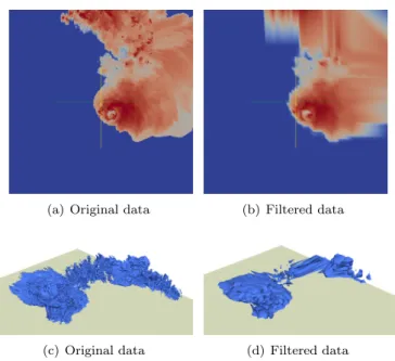
Figure 1(c) shows the result of in situ volume rendering of the reflectivity (dBZ) field in CM1. This field corresponds to the simulated radar reflectivity. It derives from a calculation based on cloud rain, hail, and snow microphysical variables, and it can be compared with real weather radar observations. A 45 dBZ isosurface reveals a feature called the weak echo region, which is linked to the physical onset of the storm.

2.2

Improving performance through data redistribution

Figure 1 also shows that the region of interest is very localized. Thus, some processes have more to render than others. The overall rendering time is driven by the rendering time of the process with the highest load. Since each sub-domain handled by a process can be further decomposed into multiple blocks, redistributing blocks to balance the load may improve performance.

(a) Original data (b) Filtered data

(c) Original data (d) Filtered data

Figure 1: Colormap (a,b) and volume rendering (c,d) of the reflectivity (dBZ) in the CM1 simulation when feeding the visualization pipeline with original data (a,c) and with filtered data (b,d).

2.3

Improving performance through data reduction

In Figures 1(b) and 1(d), each original 55 × 55 × 38-point block of data has been reduced to a 2×2×2-point block, keeping only corner values, before being fed to the visualization pipeline. While 50 seconds were required to produce Figure 1(c) on 400 cores of the Blue Waters supercomputer, only 1 second was required to produce Figure 1(d). Even though the loss of visual quality is evident in Figure 1(d), we confirmed with atmospheric scientists that such results can still be useful for tracking the evolution of the phenomena being studied.

2.4

Adapting to performance constraints

In our previous work [5], we showed that in situ visualization can largely increase the run time of a simulation when done in a time-partitioning manner (i.e., the simulation stops periodically to produce images). We also showed that in some situations the high cost of running in situ visualization algorithms in dedicated cores while the simulation keeps running forces the dedicated cores to skip some iterations and to reduce the frequency at which images are produced.

In this work, we address this problem by proposing performance-constrained in situ visualization. The main idea is that different blocks of data have different scientific value and that blocks that are not interesting can be filtered out in order to gain performance. Consequently, the in situ visualization pipeline will be continuously adapted to achieve the highest possible fidelity for the end user while staying close to a given visualization time, in a best-effort manner.

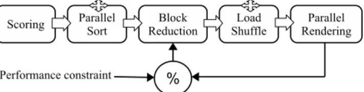
Figure 2: Overview of our performance-constrained in situ visualization ap-proach. Crosses represent steps that involve collective communications. The run time of the full pipeline is monitored at each iteration and used to control the percentage of blocks that have to be reduced.

3

Performance-Constrained In Situ Visualization

This section presents our approach to performance-constrained in situ visual-ization. We first give an overview of the approach, then discusse each of its steps: how to give a score to blocks of data, how to reduce blocks with a low score, how we redistribute the load, and finally how to adapt the pipeline to meet performance constraints.

3.1

Overview of our approach

In the following, we call the full 3D array produced by the simulation at a given iteration the domain. We call a subarray of a domain handled by one process a subdomain. We call a subarray of a subdomain a block. The number of blocks per subdomain is constant across processes. The size of all blocks is also constant.

Figure 2 illustrates our approach to performance-constrained in situ visu-alization. Given an input data divided into blocks and distributed across pro-cesses, our pipeline consists of six steps.

1. Blocks of data are scored by using a generic or user-provided metric eval-uating their relevance to either the scientific phenomenon studied or the visualization algorithm employed.

2. The scores are sorted across processes.

3. A percentage of blocks with the lowest scores is reduced.

4. A load redistribution takes place to redistribute the blocks in order to better balance the phenomenon of interest across processes.

5. The blocks are rendered through a visualization pipeline.

6. The run time of the above steps is measured, and the percentage of blocks to reduce is adapted in order for the next iteration to be processed in a targeted amount of time.

3.2

Scoring blocks of data

The first step in our approach consists of evaluating the potential relevance of each block of data, so that the least relevant blocks can later be filtered out to improve performance. Our main idea is to score how important it is to the scientific phenomena or to the visualization algorithm. While no universal metric exists for evaluating the relevance of data, we found that a set of generic metrics can still give a good idea of the importance.

In our scenario, atmospheric scientists rely on a combination of techniques to analyze their data. For example, they may render isosurfaces at different levels and use other 3D visualization scenarios, such as streamlines based on wind vectors, or 2D scenarios, such as the colormap shown in Figure 1(a). For these visualization scenario, to give accurate results, we are interested in keeping intact areas of high data variability. Therefore we investigated several metrics to score blocks based on their variability.

Statistics The range metric consists of computing the difference between the minimum and maximum values in a block of data. The intuition is that a block of data that spans a large range of values might be more interesting to keep than another. However, this metric will give a low score to blocks of data that present high variations but within a small range. A second metric in this category is the variance of the data in a block.

Interpolation Interpolation-based metrics consist of measuring the mean square error between the original data and a block of data rebuilt from an interpola-tion of a reduced set of values (its corners, for example). For 3D blocks, we use trilinear interpolation. Because many visualization algorithms use trilinear interpolation for rendering, this metric matches the error that a visualization algorithm will make when rendering blocks of data that have been reduced.

Entropy The entropy of a block of data is a way of measuring the amount of information contained in a block. The entropy is obtained by building a histogram of the values found in a block of data, and by computing E = −P pilog2(pi), where pi represents the probability of a single value in the block

to fall into bin i of the histogram. In order to be comparable across blocks, the same parameters (range and number of bins) should be used for the his-togram across all processes. Doing so requires working with a variable that falls in a known range (this is the case for the reflectivity, which falls in the range [−60, 80]) and knowing this range in advance. The number of bins can be more difficult to tune, however. In our experiments we used 256 bins. We also considered the local entropy (entropy computed at each point using a local neighborhood) as a possible metric, but this metric turned out to consume too much time relative to the duration of other components of our pipeline. We used the ITL library [3] to implement entropy-based filters.

Bytewise entropy We implemented a Lightweight Entropy Analyzer (LEA) to cope with the limitations of the classical way of computing the entropy. LEA considers each float (or double) as an array of 4 bytes (resp. 8 bytes). It then computes independently the entropy of the first byte of all float values, then

the entropy of the second byte, and so on, returning the sum of these entropies as a score. This method does not require tuning an histogram; since each byte can take 256 values, the probability pi of a value i is simply its frequency of

appearance.

Compressors We also evaluated compression algorithms as a means of scor-ing blocks of data. Our intuition is that the compression ratio should correlate with the amount of information contained in a block. Compressors do not re-quire extra information such as histogram parameters. We used the FPZIP [14], ZFP [13], and LZ [7] floating-point compressors, with different tunings for each (such as different levels or lossiness/precision). FPZIP and ZFP also have knowl-edge of the fact that blocks are 3D arrays; thus we can expect them to take locality into account. Because of space constraints, we present the results of FPZIP only. The results obtained with ZFP and LZ are similar.

We do not claim that any of these filters gives an absolute answer to the question of whether a block of data is interesting, the notion of interesting being subjective and tied to both the field of study and the visualization scenario. We provide this set of filters only as a starting point, and we rely on interactions with domain scientists to find which filter is the most appropriate for the phenomenon studied.

While we evaluated 30 filters (or variants of filters) in our experiments, we show results only for a representative subset of them: RANGE (range metric), VAR (variance), ITL (entropy), LEA (bytewise entropy), FPZIP (floating-point compression), and TRILIN (trilinear interpolation).

3.3

Sorting and reducing blocks

After each block has been given a score, the sets of pairs <id, score> are globally sorted by increasing scores (two blocks with the same score are sorted by id). The resulting sorted array is broadcast back to all processes so that each process knows the scores of all blocks including those belonging to other processes.

Based on this set, the p percent blocks with the lowest score are reduced. This reduction step consists simply of keeping the 8 corners of 3D blocks (4 corners for 2D blocks) and their coordinates. In our use case, 55 × 55 × 38-point blocks are reduced to 2×2×2 points. The percentage p of blocks to reduce is set to 0 for the first iteration and dynamically adapted later based on performance constraints.

The reason for reducing blocks this way, rather than keeping a single point with an average value, for example, is that a reduced block should still be connected to its neighboring blocks. Keeping two points along each dimension allows us to retain the extents of a blocks. Keeping the values of these points allows a continuity with neighboring blocks. Visualization algorithms will also be able to rebuild more points if necessary using interpolation from these 2×2×2 points. As can be seen in Figure 1(b), reduced blocks in a region of high variability come out blurry as a result of such interpolation.

3.4

Load redistribution (shuffling)

As a result of block reductions, the amount of data can become imbalanced across processes. Blocks with a high score (therefore not reduced) are indeed

likely to be clustered in a small region handled by a reduced number of processes. This imbalance adds up to the imbalance of rendering load, defined as the time required for a piece of data to be rendered. Even if none of the blocks are reduced, the locality of the physical phenomena and the resulting isosurface lead to some processes having more rendering load than others.

This situation may impair the performance of the final rendering step. In particular the total run time of the rendering step is driven by the run time of its slowest process, that is, the process with the highest load.

In order to gain performance, the blocks must be redistributed across pro-cesses. Since process rank 0 already broadcasts the scores of all blocks to all processes, all processes have the same full, sorted list of blocks. Upon reading this list, each process issues a series of nonblocking receives to get blocks that they need, and a series of nonblocking sends to send blocks to other processes.

We implement two load redistribution strategies.

• Random Shuffling Each process is given the responsibility for a random set of blocks (the number of blocks per process remains constant). The redistribution of blocks is computed the same way in all processes by making sure all processes use the same seed. This strategy constitutes our baseline; it does not take the scores into account, and it does not attempt to optimize communications.

• Round Robin The blocks, sorted by their score, are distributed across processes in a round-robin manner. That is, process 0 takes the block with the highest score; process 1 the block with the second highest score, and so on, looping over processes until no more blocks remain to be dis-tribute. This strategy takes the scores into account but does not attempt to optimize communications.

Our experiments show that such communications have a negligible overhead, on the order of 1 second, on the target platform (Blue Waters) compared with the rendering time, on the order of tens to hundreds of seconds.

3.5

Adapting to performance constraints

The last step in our approach consists of dynamically adapting the number of blocks that are reduced based on predefined performance constraints. In our case the performance constraint is the maximum run time for the full pipeline to complete.

To implement this adaptive reduction of data, we assume that (1) for a given iteration n, the total run time of the pipeline is a monotonically increasing function fn of the number of nonreduced blocks and (2) for every iteration n,

fn−1is a good approximation of fn.

Assumption (1) is intuitive, given that all parts of the pipeline either do not depend on the number of reduced blocks (the scoring component and parallel sort) or benefit from the reduction (load redistribution and rendering).

Assumption (2) may not always be true, especially because the performance of the rendering pipeline is inherently variable, and because the rendering load varies as the physical phenomenon evolves (for example, if a cloud gets bigger, it spans more domains and requires more time to be rendered). It may happen that although we increase the percentage of reduced blocks from iteration n − 1

Algorithm 1 Computes the percentage of blocks to reduce based on the per-centages used for the two previous iterations (pn−1 and pn) and the observed

timings (tn−1and tn). target is the required run time of the full pipeline.

1: function adapt_percent(target, tn−1, pn−1, tn, pn)

2: if pn−1= pn then . Deal with a vertical slope

3: if tn > targetand pn< 100 then return pn+ 1

4: end if

5: if tn < targetand pn> 0 then return pn− 1

6: end if

7: end if

8: . Compute linear estimation, i.e., we find a and b such that t = a × p + b

9: a ← tn−tn−1

pn−pn−1

10: b ← tn− a × pn

11: if a ≥ 0 then return min(100, pn+ 1) . May happen because of

randomness in rendering time.

12: end if

13: p ← target−b_a . Estimate next percentage

14: returnmin(100,max(p,0)) . Make sure p is in [0,100]

15: end function

to iteration n (which should lead to a decrease of run time), the rendering time increases as well because fn−1 was not a good approximation of fn. Our

algorithm takes this case into account by simply increasing the percentage by 1 instead of decreasing the percentage of reduced blocks in the hope of decreasing the run time.

Algorithm 1, our solution to the above problem, starts by assuming that the rendering time t0 when all blocks are reduced is t0 = 0. The first output of

the simulation is not reduced (p1 = 0), and leads to a time t1. After the first

iteration, we always keep the rendering time and percentages of the two previous iterations (tn−1, pn−1, tn, pn), and compute an estimate of the rendering time

as a function of the percentage. This linear approximation allows us to get the next percentage pn+1 required to reach the target run time. Lines 2 to 7

prevent our algorithm from being stuck because it used the same percentage two iterations in a row. The case of Assumption (2) being broken is handled in line 10. Line 13 makes sure that the resulting value stays within [0, 100].

4

Experimental evaluation

In this section, we evaluate all the components of our pipeline individually and together. After describing the experimental setup, we divide our evaluation into several parts, each focusing on a single component of the pipeline. The last part is the overall performance gain.

4.1

Description of the experiments

We demonstrate the benefit of our approach through experiments with the CM1 application on NCSA’s Blue Waters petascale supercomputer [19]. We focus

0 10 20 30 40 50 60 70 80 LEA

FPZIP ITL_RANGE VARTRILIN

Filter Performance (MB/s)

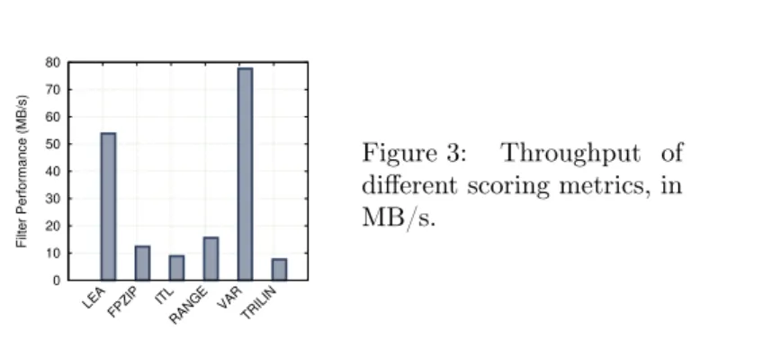
Figure 3: Throughput of different scoring metrics, in MB/s.

in particular on the reflectivity field produced by CM1. While the colormap visualization scenario is already fast (on the order of a second to complete), rendering the isosurface can take several minutes. We therefore focus on this scenario specifically. The colormap will, however, be used to show how the scores given by different metrics map to certain regions of the data.

In our previous work we used Damaris/Viz and VisIt to enable in situ vi-sualization in CM1. In the present work, we use ParaView Catalyst instead, since it allows us to define various batch visualization pipelines through Python scripts.

To avoid running CM1’s computational part for every experiment, and be-cause interesting phenomena start to appear only after a few thousand itera-tions, we use a dataset already generated by atmospheric scientists. This dataset consists of 572 iterations of data (starting after approximately 5,000 iterations of the simulation), each a 2200 × 2200 × 380 array of 32-bit floating-point val-ues representing the reflectivity on each point of a 3D rectilinear grid. It was generated from a 3-day run of CM1 on Blue Waters. We reloaded this dataset using the Block I/O Library (BIL) [10] into an in situ visualization kernel of CM1 that feeds it to a Catalyst pipeline.

We use 10 iterations, equally spaced in time, to evaluate our approach, ex-cept when evaluating the self-adaptation mechanism, in which case we use 30 iterations. We run our experiments on 64 cores (4 nodes) and 400 cores (25 nodes). In both cases, the data is initially read and distributed across processes the same way CM1 would have generated it at these scales.

4.2

Score metrics: performance and relevance

We compared our block-scoring metrics in several ways. First, we measured how fast these metrics score blocks. Figure 3 shows their respective throughput. Table 1 presents the corresponding computation time on 64 and 400 cores, with 16,000 blocks of 55 × 55 × 38 floating-point values. These times must be put in perspective with the rendering time. For example, on 64 cores it takes about 160 seconds to render all the blocks without reducing any of them. Using the TRILIN function adds 14.3 seconds to this run time, which, in our opinion, is not acceptable for a function that aims only at guiding a later selection of blocks. We therefore prefer a scoring function such as LEA or VAR, which only take 2.03 and 1.41 seconds, respectively.

The second aspect of the metrics that has to be studied is how they rank blocks compared with one another. Since our approach consists of selecting a percentage of blocks with the highest score, two metrics may not select the same

Table 1: Computation time required for different metrics. Metric Time on 64 cores (sec) Time on 400 cores (sec)

LEA 2.03 0.325 FPZIP 8.85 1.416 ITL 13.3 1.972 RANGE 7.03 1.125 VAR 1.41 0.226 TRILIN 14.3 2.285 blocks.

In Figure 4, each graph compares a pair of metrics. Each point on a graph represents a block. The abscissa of the point represents the rank of the block when blocks are sorted according to the first metric. Its ordinate represents the rank of the block when blocks are sorted according to the second metric.

From these figures we can clearly see a set of blocks that all metrics “agree” are not variable enough to be considered relevant. The scores of these blocks is the minimum score that the metrics can give; therefore they are sorted by id rather than by score, leading to the same order according to all metrics. For blocks that present more variability, the metrics tend to disagree on the ordering. This is an expected result because each metric evaluates a different aspect of variability. Some relations between metrics can yet be highlighted, such as the fact that a large entropy with ITL seems to imply a large variance, while the opposite mays not be true, and the fact that the trilinear interpolation score seems to correlate well with the variance, which may come from the fact that in both cases a mean square error with respect to a reference value (for the variance) or function (for trilinear interpolation) is computed.

To guide the user in choosing metrics, we display an image (such as the colormap presented in Section 2) and show how each block part of the image is scored. This kind of 2D visualization is easy to compute and fast; it can also be done offline with samples of data from previous runs of the simulation.

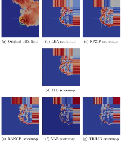
Figure 5 shows score maps, that is, colormaps of the domain where colors represent scores of blocks, and compares them to the original reflectivity field. It shows that some metrics such as VAR or TRILIN give a higher score to regions with larger overall variability (e.g., contours of the phenomenon) while other such as ITL or FPZIP also give a high score to blocks inside the phenomenon itself. Note that the longer blocks on the borders of the domain are due to the simulation grid, which is rectilinear. These blocks have the same number of points as any other.

Informal discussions with atmospheric scientists indicated that they were particularly interested in the vortex region at the center of the domain (this regions is circled in green in Figure 5) When being shown the scoremaps in Figure 5 for feedback, their interest turned to the VAR and TRILIN metrics, which seem to give a high score to this region while giving a low score to its surrounding.

(a) LEA vs FPZIP (b) LEA vs ITL (c) LEA vs RANGE

(d) LEA vs VAR (e) LEA vs TRILIN (f) FPZIP vs ITL

(g) FPZIP vs RANGE (h) FPZIP vs VAR (i) FPZIP vs TRILIN

(j) ITL vs RANGE (k) ITL vs VAR (l) ITL vs TRILIN

(m) RANGE vs VAR (n) RANGE vs TRILIN (o) VAR vs TRILIN

Figure 4: Comparison of block orderings produced by various metrics. Each graph compares two metrics. Each point represents a block. The abscissa of the point represents the rank of the block when the blocks are sorted according to the first metric. The ordinate of the point is the rank of the block when sorted

(a) Original dBZ field (b) LEA scoremap (c) FPZIP scoremap

(d) ITL scoremap

(e) RANGE scoremap (f) VAR scoremap (g) TRILIN scoremap

0 20 40 60 80 100 120 140 160 180 200 NONE SHUFFLE LEA

FPZIP ITL_RANGEVARTRILIN

Rendering Time (sec)

(a) 64 cores 0 10 20 30 40 50 60 NONE SHUFFLE LEA

FPZIP ITL_RANGEVARTRILIN

Rendering Time (sec)

(b) 400 cores

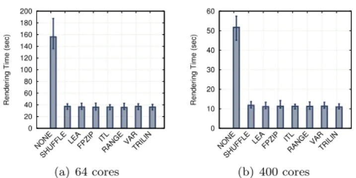
Figure 6: Run time of the rendering pipeline when none of the blocks are re-duced, but load-redistribution is enabled based on scores provided by different metrics. NONE represent the case where the load has not been redistributed, SHUFFLE corresponds to random shuffling, and all others correspond to a round-robin distribution according to scores.

4.3

Performance benefit of load redistribution

We then confirmed that redistributing the blocks to divide the cost of the physi-cal phenomena benefits the rendering performance. To do so, we ran our pipeline without load redistribution, with random load redistribution and with load re-distribution in a round-robin fashion according to different metrics. Figure 6 shows the rendering time in these experiments. The communication time is 1.2 seconds on 64 cores and 0.6 seconds on 400 cores, both for the random shuffling strategy and the round-robin policy.

These results show that simply by redistributing the load, we can achieve a 5×speedup on 400 cores and a 4× speedup on 64 cores. It also shows that there is no benefit in taking the scores into account; randomly redistributing blocks already achieves a good statistical load balancing because of the relatively small size of the phenomena of interest compared with the size of the full domain. Section 4.5 studies the interaction of the load redistribution component and the block reduction component.

4.4

Performance benefit of block reduction

In the next series of experiments we evaluate how much performance is gained by reducing a certain percentage of the blocks, and we show how the run time evolves as a function of the percentage of blocks being reduced. We arbitrarily used the TRILIN metric (other metrics yield similar results) to score blocks of data.

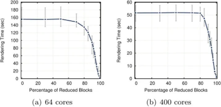
Figure 7 shows the run time of 10 iterations for different percentages of blocks being reduced. When none of the blocks are reduced, the run time is 160 seconds on 64 cores and 50 seconds on 400 cores. When all the blocks are reduced, this run time goes down to 1 second in both cases. This defines the margins within which we can adapt the performance by changing the number of blocks being reduced when load redistribution is not involved.

This figure also shows that the rendering time is not the same from one iteration to another. As will be shown later, this variability will affect our

0 20 40 60 80 100 120 140 160 180 200 0 2 4 6 8 10

Rendering Time (sec)

Iteration Number 0 percent 80 percent 90 percent 98 percent 100 percent (a) 64 cores 0 10 20 30 40 50 60 0 2 4 6 8 10

Rendering Time (sec)

Iteration Number 0 percent 90 percent 94 percent 98 percent 100 percent (b) 400 cores

Figure 7: Run time of the rendering pipeline for 10 iterations, with different percentages of blocks being reduced.

0 20 40 60 80 100 120 140 160 180 200 0 20 40 60 80 100

Rendering Time (sec)

Percentage of Reduced Blocks

(a) 64 cores 0 10 20 30 40 50 60 0 20 40 60 80 100

Rendering Time (sec)

Percentage of Reduced Blocks

(b) 400 cores

Figure 8: Run time of the rendering pipeline (average, minimum, and maximum across 10 iterations) as a function of the percentage of blocks being reduced.

adaptation algorithm.

Figure 8 presents the same results as a function of the percentage of reduced blocks, with error bars representing minimum and maximum across the 10 it-erations. We observe that the performance improvement is not proportional to the percentage of reduced blocks. Instead, a majority of the blocks need to be reduced before we start observing performance improvements. The reason is that the selection of blocks to be reduced is based on their score, yet blocks with a high score are not evenly distributed across processes. Hence a few processes are likely to have a large number of high-scored blocks and will not see their load being reduced until the percentage is high enough that we start selecting their blocks too.

4.5

Combined reduction and load redistribution

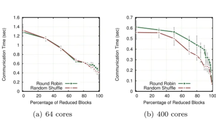
Data reduction has a potential impact on the time to perform load redistribu-tion. Indeed, since data is reduced before being redistributed, reducing more blocks means exchanging less data. Although this redistribution time is negli-gible compared with the rendering time, we show in Figure 9 how it evolves as a function of the number of blocks being reduced. For this set of experiments we used the LEA metric. As expected, the communication time decrease as we

0 0.2 0.4 0.6 0.8 1 1.2 1.4 1.6 0 20 40 60 80 100

Communication Time (sec)

Percentage of Reduced Blocks Round Robin Random Shuffle (a) 64 cores 0 0.1 0.2 0.3 0.4 0.5 0.6 0.7 0 20 40 60 80 100

Communication Time (sec)

Percentage of Reduced Blocks Round Robin Random Shuffle

(b) 400 cores

Figure 9: Run time of the redistribution component (average, minimum, and maximum across 10 iterations) as a function of the percentage of blocks being reduced. 0 20 40 60 80 100 120 140 160 180 200 0 20 40 60 80 100

Rendering Time (sec)

Percentage of Reduced Blocks No Redistribution Round Robin Random Shuffle (a) 64 cores 0 10 20 30 40 50 60 0 20 40 60 80 100

Rendering Time (sec)

Percentage of Reduced Blocks No Redistribution

Round Robin Random Shuffle

(b) 400 cores

Figure 10: Run time of the rendering component (average, minimum and max-imum across 10 iterations) as a function of the percentage of blocks being re-duced, when load redistribution is enabled or disabled.

increase the percentage of reduced blocks, as a result of a lower amount of data to be exchanged.

Load redistribution combined with data reduction have an effect on the rendering performance. This effect is shown in Figure 10. It shows that load redistribution not only improves performance but it also reduces the variability of the rendering tasks.

Additionally, Figure 10 shows that the round-robin and random policies lead to the same performance of the rendering task; that is, a score-guided redistri-bution achieves a load balancing equivalent to the statistical load balancing.

4.6

Dynamic adaptation

We first evaluate our dynamic adaptation technique without the redistribution component. We then add the redistribution component to show the resulting performance of the entire pipeline.

4.6.1 Adaptation without redistribution

In this set of experiments, we set a target run time of 120, 60, and 20 seconds per iteration on 64 cores, and 30, 15, and 7 seconds on 400 cores. Figures 11(a) and 11(b) present the resulting run time for 30 iterations. They show that our approach can successfully adapt the percentage of reduced blocks in order to reach a target run time per iteration. Figures 11(c) and 11(d) show that the percentages have stabilized after a few iterations. The variability observed in the run time comes from the inherent variability of the visualization task.

4.6.2 Adaptation with redistribution enabled

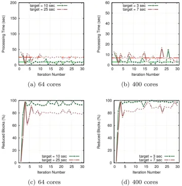
We evaluate the full pipeline, including load redistribution, with dynamic adap-tation. Figure 12 presents the resulting run time for 30 iterations. Here the target run time is 25 and 10 seconds per iteration on 64 cores and 7 and 3 seconds per iteration on 400 cores. We used the same scale for the y axis as in Figure 11 so that Figures 11 and 12 can be compared. These results show that our pipeline not only improves performance but it can also meet performance constraints despite the variability of the rendering task.

5

Related work

In the following we present related work in the field of in situ visualization and in particular techniques that attempt to adapt the in situ visualization pipelines.

5.1

In situ visualization frameworks

In the past few years, several approaches to in situ visualization have been pro-posed by the community and have consequently led to the addition of in situ capabilities in existing software. One trend has been to offer an in situ visual-ization API to connect simulations to visualvisual-ization software such as VisIt [15] through its libsim library [24] or ParaView [11] through its coprocessing/Cata-lyst library [6].

Another approach to in situ visualization has been to modify the I/O stack rather than the simulation itself. This trend is driven mainly by the ADIOS [16] community and the variety of work that revolves around this I/O interface, including PreDatA [26], which uses a staging area of dedicated nodes to per-form data analytics, or GLEAN [22], which integrates time-partitioning data-processing capabilities at the simulation and staging area with an emphasis on architecture awareness.

The Damaris/Viz approach [5] has been proposed to extend the Damaris middleware [4, 8] in the context of in situ visualization. Although Damaris was initially designed to offer data management capabilities through dedicated cores using shared memory for intranode data movements, it now can run in time-partitioning mode and deploy a staging area in dedicated nodes as well. The use of dedicated cores for in situ data processing and analytics can also be found in other works [12, 25].

Many other approaches to in situ visualization have been proposed [5, 20, 18]. All these approaches and frameworks are driving a shift from offline analysis to in situ analysis and visualization. Yet none of them self-adapts to the visualization

0 20 40 60 80 100 120 140 160 180 200 0 5 10 15 20 25 30

Rendering Time (sec)

Iteration Number target = 120 sec target = 60 sec target = 20 sec (a) 64 cores 0 10 20 30 40 50 60 0 5 10 15 20 25 30

Rendering Time (sec)

Iteration Number target = 30 sec target = 15 sec target = 7 sec (b) 400 cores 0 20 40 60 80 100 0 5 10 15 20 25 30 Reduced Blocks (%) Iteration Number target = 120 sec target = 60 sec target = 20 sec (c) 64 cores 0 20 40 60 80 100 0 5 10 15 20 25 30 Reduced Blocks (%) Iteration Number target = 30 sec target = 15 sec target = 7 sec (d) 400 cores

Figure 11: Rendering time (a+b) and percentage of blocks reduced (c+d) on 64 and 400 cores when trying to converge toward a specified run time. Load redistribution is not activated here.

0 50 100 150 200 0 5 10 15 20 25 30

Processing Time (sec)

Iteration Number target = 10 sec target = 25 sec (a) 64 cores 0 10 20 30 40 50 60 0 5 10 15 20 25 30

Processing Time (sec)

Iteration Number target = 3 sec target = 7 sec (b) 400 cores 0 20 40 60 80 100 0 5 10 15 20 25 30 Reduced Blocks (%) Iteration Number target = 10 sec target = 25 sec (c) 64 cores 0 20 40 60 80 100 0 5 10 15 20 25 30 Reduced Blocks (%) Iteration Number target = 3 sec target = 7 sec (d) 400 cores

Figure 12: Full pipeline (including load redistribution) completion time (a+b) and percentage of blocks reduced (c+d) on 64 and 400 cores when trying to converge toward a specified run time.

payload and the content of the data to reach a targeted performance. Their analysis/visualization pipeline is fixed and does not attempt to reduce the data volume at the source nor redistribute data. Our work is novel in this aspect. We also note that, although we choose to apply it to the Catalyst framework, it can be applied to any of the other aforementioned frameworks, some of which would enable further improvements. The use of dedicated cores or nodes in Damaris would, for example, allow the load redistribution to be done simply by having clients change the Damaris server they interact with. The capabilities for an in situ visualization framework to select relevant subsets of data to be stored or visualized is mentioned as one of the design issues for in situ visualization by Thompson et al. [21].

5.2

Adaptive in situ visualization

More and more efforts are put into designing in situ visualization frameworks that adapt to the content of the data (for instance, its compressibility) or to the availability of resources such as local memory.

Zou et al. [27] presented an in situ visualization framework based on EVpath that takes into account the quality of information (QoI) as well as the quality of service (QoS). Their QADMS approach applies lossy compression selectively depending on a tradeoff between QoI (defined as the ratio between compressed data size and original data size) and QoS (defined as the end-to-end latency). While they lay the foundation of data reduction for in situ visualization, our ap-proach is different in that our data reduction method consists of removing entire blocks (keeping the corners) rather than lossy-compressing the full set of points. Since the number of points in their approach does not change, the rendering time remains the same, and only the data transfer between the simulation and a staging area is improved. Our approach improves both data redistribution and rendering time.

Malakar at al. [17] introduced an in situ visualization framework in which data is sent from the simulation to a visualization cluster at a frequency that is dynamically adapted to resource constraints. This approach tries to maximize the temporal accuracy (i.e., by maximizing the frequency of in situ visualization updates) but keeps a fixed spatial resolution. Our approach proposes to adapt the spatial resolution as well and to do it selectively on chunks of data considered relevant.

Jin et al. [9] proposed to adapt the in situ visualization process either by adapting the resolution at which the data is rendered or by changing the lo-cation of the rendering tasks (using either in situ visualization or in transit visualization). To adapt the resolution of the data, they used entropy-based downsampling. We proposed and evaluated several other metrics, in particular based on the use of floating-point compressors. Additionally, we investigated the impact of data redistribution on such metrics.

Closer to our work is the work by Wang et al. [23], who proposed finding importantdata in time-varying datasets by using information theory metrics and by looking at the evolution of such metrics across different time steps. Although their work provides key insights into defining the importance of a piece of data, their solution is not applied in situ, that is, in a context where the performance of filtering relevant data is extremely important to avoid any impact on the running simulation.

6

Conclusion

While in situ visualization enables faster insight into a running simulation, it can increase the simulation’s run time and increase its variability. Needed, therefore, are ways to improve the performance of in situ visualization, as well as to make its task fit in a given performance budget, even at the cost of reduced visual accuracy.

In this paper, we have addressed the challenge of improving in situ visual-ization performance in the context of a climate simulation. We realized that the strong locality of the phenomenon of interest limits the performance of a normal rendering pipeline. Hence, we proposed redistributing blocks of data and reducing a percentage of them based on their content. Additionally, we proposed adapting the percentage so that our pipeline adheres to performance constraints. We have shown that our pipeline can speed the visualization time by 5× on 400 cores without affecting the visual results, and that it can effectively meet given performance constraints provided that data reduction is allowed.

We plan to investigate whether more elaborate redistribution algorithms are necessary in order to achieve the same results at larger scale and on platforms with lower network performance. We will also investigate multivariate scores and other visualization scenarios tied to other field variables of CM1 and other simulations.

Acknowledgments

This material is based upon work supported by the U.S. Department of Energy, Office of Science, Office of Advanced Scientific Computing Research, under contract number AC02-06CH11357. This work is also supported by DOE with agreement No. DE-DC000122495, program manager Lucy Nowell.

References

[1] A. C. Bauer, B. Geveci, and W. Schroeder. The ParaView Catalyst UserâĂŹs Guide v2.0. Kitware, Inc. http://www.paraview.org/files/catalyst/ docs/ParaViewCatalystUsersGuide-v2.pdf, 2015.

[2] G. H. Bryan and J. M. Fritsch. A Benchmark Simulation for Moist Nonhydrostatic Numerical Models. Monthly Weather Review, 130(12):2917–2928, 2002.

[3] A. Chaudhuri, T.-Y. Lee, B. Zhou, C. Wang, T. Xu, H.-W. Shen, T. Peterka, and Y.-J. Chiang. Scalable Computation of Distributions from Large Scale Data Sets. In Proceedings of the 2012 IEEE Large Data Analysis and Visualization Symposium LDAV’12, Seattle, WA, 2012.

[4] M. Dorier, G. Antoniu, F. Cappello, M. Snir, and L. Orf. Damaris: How to Efficiently Leverage Multicore Parallelism to Achieve Scalable, Jitter-free I/O. In IEEE International Conference on Cluster Computing (CLUSTER), pages 155 –163, Sept. 2012.

[5] M. Dorier, R. Sisneros, Roberto, T. Peterka, G. Antoniu, and B. Semeraro, Dave. Damaris/Viz: a Nonintrusive, Adaptable and User-Friendly In Situ Visualization Framework. In LDAV - IEEE Symposium on Large-Scale Data Analysis and Visualization, Atlanta, GA, USA, Oct. 2013.

[6] N. Fabian, K. Moreland, D. Thompson, A. Bauer, P. Marion, B. Geveci, M. Rasquin, and K. Jansen. The ParaView Coprocessing Library: A Scalable,

General Purpose In Situ Visualization Library. In LDAV, IEEE Symposium on Large-Scale Data Analysis and Visualization, 2011.

[7] L. Gomez and F. Cappello. Improving Floating Point Compression through Bi-nary Masks. In IEEE International Conference on Big Data, pages 326–331, Oct. 2013.

[8] INRIA. Damaris, http://damaris.gforge.inria.fr/.

[9] T. Jin, F. Zhang, Q. Sun, H. Bui, M. Parashar, H. Yu, S. Klasky, N. Podhorszki, and H. Abbasi. Using cross-layer adaptations for dynamic data management in large scale coupled scientific workflows. In Proceedings of the International Conference on High Performance Computing, Networking, Storage and Analysis, SC ’13, pages 74:1–74:12, New York, NY, USA, 2013. ACM.

[10] W. Kendall, J. Huang, T. Peterka, R. Latham, and R. Ross. Visualization View-point: Towards a General I/O Layer for Parallel Visualization Applications. IEEE Computer Graphics and Applications, 31(6), 2011.

[11] KitWare. ParaView, http://www.paraview.org/.

[12] M. Li, S. S. Vazhkudai, A. R. Butt, F. Meng, X. Ma, Y. Kim, C. Engelmann, and G. Shipman. Functional Partitioning to Optimize End-to-End Performance on Many-core Architectures. In Proceedings of the 2010 ACM/IEEE International Conference for High Performance Computing, Networking, Storage and Analysis, SC’10, pages 1–12, Washington, DC, USA, 2010. IEEE Computer Society. [13] P. Lindstrom. Fixed-Rate Compressed Floating-Point Arrays. IEEE Transactions

on Visualization and Computer Graphics, 20(12):2674–2683, Dec 2014.

[14] P. Lindstrom and M. Isenburg. Fast and Efficient Compression of Floating-Point Data. IEEE Transactions on Visualization and Computer Graphics, 12(5):1245– 1250, Sept 2006.

[15] LLNL. VisIt, https://wci.llnl.gov/codes/visit/.

[16] J. F. Lofstead, S. Klasky, K. Schwan, N. Podhorszki, and C. Jin. Flexible IO and integration for scientific codes through the adaptable IO system (ADIOS). In Proceedings of the 6th international workshop on Challenges of large applications in distributed environments, CLADE ’08, pages 15–24, New York, NY, USA, 2008. ACM.

[17] P. Malakar, V. Natarajan, and S. S. Vadhiyar. An Adaptive Framework for Simulation and Online Remote Visualization of Critical Climate Applications in Resource-constrained Environments. In Proceedings of the 2010 ACM/IEEE International Conference for High Performance Computing, Networking, Storage and Analysis, SC’10, pages 1–11, Washington, DC, USA, 2010. IEEE Computer Society.

[18] K. Moreland, R. Oldfield, P. Marion, S. Jourdain, N. Podhorszki, V. Vishwanath, N. Fabian, C. Docan, M. Parashar, M. Hereld, et al. Examples of In Transit Visualization. In Proceedings of the 2nd international workshop on Petascal data analytics: challenges and opportunities, pages 1–6. ACM, 2011.

[19] NCSA. Blue Waters project. http://www.ncsa.illinois.edu/

BlueWaters/.

[20] M. Rivi, L. Calori, G. Muscianisi, and V. Slavnic. In-situ visualization: State-of-the-art and some use cases. PRACE White Paper (2012), http://www. prace-ri. eu/Visualisation, 2011.

[21] D. Thompson, N. Fabian, K. Moreland, and L. Ice. Design Issues for Performing In Situ Analysis of Simulation Data. Technical report, Technical Report SAND2009-2014, Sandia National Laboratories, 2009.

[22] V. Vishwanath, M. Hereld, V. Morozov, and M. E. Papka. Topology-Aware Data Movement and Staging for I/O Acceleration on Blue Gene/P Supercomputing Systems. In Proceedings of 2011 International Conference for High Performance Computing, Networking, Storage and Analysis, SC’11, pages 19:1–19:11, New York, NY, USA, 2011. ACM.

[23] C. Wang, H. Yu, and K.-L. Ma. Importance-Driven Time-Varying Data Visualiza-tion. IEEE Transactions on Visualization and Computer Graphics, 14(6):1547– 1554, Nov. 2008.

[24] B. Whitlock, J. M. Favre, and J. S. Meredith. Parallel In Situ Coupling of Simula-tion with a Fully Featured VisualizaSimula-tion System. In Eurographics Symposium on Parallel Graphics and Visualization (EGPGV). Eurographics Association, 2011. [25] F. Zhang, C. Docan, M. Parashar, S. Klasky, N. Podhorszki, and H. Abbasi.

Enabling in-situ execution of coupled scientific workflow on multi-core platform. Parallel and Distributed Processing Symposium, International, pages 1352–1363, 2012.

[26] F. Zheng, H. Abbasi, C. Docan, J. Lofstead, Q. Liu, S. Klasky, M. Parashar, N. Podhorszki, K. Schwan, and M. Wolf. PreDatA - Preparatory Data Ana-lytics on Peta-Scale Machines. In IEEE International Symposium on Parallel Distributed Processing (IPDPS), pages 1–12, April 2010.

[27] H. Zou, F. Zheng, M. Wolf, G. Eisenhauer, K. Schwan, H. Abbasi, Q. Liu, N. Pod-horszki, and S. Klasky. Quality-aware data management for large scale scientific applications. In SC Companion: High Performance Computing, Networking, Stor-age and Analysis (SCC), pStor-ages 816–820, Nov. 2012.

The submitted manuscript has been created by UChicago Argonne, LLC, Operator of Argonne National Laboratory ("Argonne"). Argonne, a U.S. De-partment of Energy Office of Science laboratory, is operated under Contract No. DE-AC02-06CH11357. The U.S. Government retains for itself, and others acting on its behalf, a paid-up nonexclusive, irrevocable worldwide license in said arti-cle to reproduce, prepare derivative works, distribute copies to the public, and perform publicly and display publicly, by or on behalf of the Government.