HAL Id: hal-02364093
https://hal-univ-rennes1.archives-ouvertes.fr/hal-02364093
Submitted on 11 Dec 2019
HAL is a multi-disciplinary open access
archive for the deposit and dissemination of
sci-entific research documents, whether they are
pub-lished or not. The documents may come from
teaching and research institutions in France or
abroad, or from public or private research centers.
L’archive ouverte pluridisciplinaire HAL, est
destinée au dépôt et à la diffusion de documents
scientifiques de niveau recherche, publiés ou non,
émanant des établissements d’enseignement et de
recherche français ou étrangers, des laboratoires
publics ou privés.
Temporally downsampled cerebral CT perfusion image
restoration using deep residual learning
Haichen Zhu, Dan Tong, Lu Zhang, Shijie Wang, Weiwen Wu, Hui Tang,
Yang Chen, Limin Luo, Jian Zhu, Baosheng Li
To cite this version:
Haichen Zhu, Dan Tong, Lu Zhang, Shijie Wang, Weiwen Wu, et al.. Temporally downsampled cerebral
CT perfusion image restoration using deep residual learning. International Journal of Computer
Assisted Radiology and Surgery, Springer Verlag, 2020, 15 (2), pp.193-201.
�10.1007/s11548-019-02082-1�. �hal-02364093�
Temporally Downsampled Cerebral CT Perfusion
Image Restoration Using Deep Residual Learning
Haichen Zhu1,#, Dan Tong2,#, Lu Zhang3, Shijie Wang1, Weiwen Wu4, Hui Tang1, Yang Chen1,5,*,
Limin Luo1, Jian Zhu6, Baosheng Li6
1 Lab of Image Science and Technology, Key Laboratory of Computer Network and Information Integration (Ministry of Education), Southeast University, Nanjing 210096, China 2 Department of Radiology, The First Hospital of Jilin University, Changchun 130021, China
3 IETR, CNRS UMR 6164, INSA Rennes, Rennes 35708, France
4 Key Lab of Optoelectronic Technology and Systems, Ministry of Education, Chongqing University, Chongqing 400044, China
5 Centre de Recherche en Information Biomedicale Sino-Francais (LIA CRIBs), 35000 Rennes, France 6 Department of Radiation Oncology, Shandong Cancer Hospital, Shandong University, Jinan 250117,
China
#: These authors contributed equally to this study * Yang Chen [email protected]
Abstract
Purpose
Acute ischemic stroke is one of the most causes of death all over the world. Onset to treatment time is critical in stroke diagnosis and treatment. Considering the time consumption and high price of MR imaging, CT perfusion (CTP) imaging is strongly recommended for acute stroke. However, too much CT radiation during CTP imaging may increase the risk of health problems. How to reduce CT radiation dose in CT perfusion imaging has drawn our great attention.Method
In this study, the original 30-pass CTP images are downsampled to 15 passes in time sequence, which equals to 50% radiation dose reduction. Then, a residual deep convolutional neural network (CNN) model is proposed to restore the downsampled 15-pass CTP images to 30 passes to calculate the parameters such as CBF (Cerebral Blood Flow), CBV (Cerebral Blood Volume), MTT (Mean Transit Time), TTP (Time To Peak) for stroke diagnosis and treatment. The deep restoration CNN network is implemented simply and effectively with 16 successive convolutional layers which form a wide enough receptive field for input image data. 18 patients’ CTP images are employed as training set and the other 6 patients’ CTP images are treated as test dataset in this study.Results
Experiments demonstrate that our CNN network can restore high-quality CTP images in terms of structural similarity index (SSIM) and peak signal-to-noise ratio (PSNR). The average SSIM and PSNR for test images are 0.981 and 56.25, and the SSIM and PSNR of regions of interest (ROI) are 0.915 and 42.44 respectively, showing promising quantitative level. In addition, we compare the perfusion maps calculated from the restored images and from the original images, and the average perfusion results of them are extremely close.Areas of hypoperfusion of 6 test cases could be detected with comparable accuracy by radiologists.Conclusion
The trained model can restore the temporally downsampled 15-pass CTP to 30 passes very well. According to the contrast test, sufficient information cannot be restored with e.g., simple interpolation method and Deep Convolutional Generative Adversarial Network (DCGAN), but can be restored with the proposed CNN model. This method can be an optional way to reduce radiation dose during CTP imaging.Key Words:
Acute Ischemic Stroke, Low-dose CT, CT Perfusion Imaging, Deep residual CNNIntroduction
As one of leading causes of death, stroke may bring serious long-term disability. According to the statistics, there are about 2.5 million new stroke cases in China every year, and about 1.7 million patients die from stroke [1]. In acute stroke treatment, time is life. It is strongly recommended to conduct a rapid diagnosis of suspected stroke patients on the basis of the diagnostic procedure, complete the basic assessment of brain CT and start treatment within 60 minutes after reaching the emergency room as much as possible, and perform intravenous thrombolysis within 6 hours by Chinese Medical Association Cerebrovascular Disease Group [2]. Considering the drawbacks of imaging speed and expense of MRI, CT perfusion (CTP) imaging is widely used in acute stroke diagnosis in China. However, CT radiation dose has always been concerned. How to reduce radiation exposure while maintaining image quality is a key point in CT imaging, which is known as the principle of “as low as reasonably achievable (ALARA)” [3]. To reduce radiation dose and related risk of cancers, low dose CT (LDCT) has been of great research interest in CT imaging. Generally speaking, there are three typical approaches to reduce CT radiation: reducing tube current [4], sparse-view sampling [5], and region-of-interest (ROI) scanning [6]. Current brain CTP consists of about 30-pass CT images, which means scanning brain for 30 times within about 50 seconds after injecting iodinated contrast agents. Inspired by the sparse-view low-dose CT imaging, we cut down the original 30 passes to 15 passes in time sequence since it is the easiest way to reduce scan radiation for our study. Then some brain perfusion parameters such as CBF (Cerebral Blood Flow), CBV (Cerebral Blood Volume), MTT (Mean Transit Time) and TTP (Time To Peak) were calculated for clinical diagnosis. However, the missing data would lead to miscalculating brain perfusion parameters. Hence, we intended to recover 30-pass high-quality CTP images from the downsampled CTP images.
Streak artifacts usually occur in sparsely sampled low-dose CT reconstruction when using analytical methods. Interpolating the missing view can be an optional way to reduce artifacts of reconstructed sparse-view CT images [7, 8]. Recently, deep learning methods have been available for extensive computer vision tasks, such as image classification [9], semantic segmentation [10, 11], super-resolution generation [12] and medical image reconstruction [13]. As for low-dose CT imaging, H. Lee[14] and D. Lee[15] proposed some effective convolutional neural networks (CNN) to interpolate sparsely sampled CT data and reduce the streak artifacts in sinogram and image domain. More recently, a generative adversarial network (GAN) containing convolutional layer was trained to estimate routine-dose CT images from low-dose CT images [16]. Though the results showed improved performance, the application of comprehensive networks are greatly limited by the high computation cost related to the massive back-projections in network training. Besides, these networks were not developed for CTP image reconstruction task.
In this study, we proposed a simple three-dimensional convolutional neural network to interpolate the missing data to restore temporally downsampled CTP images in time sequence. Then the restored 30-pass CTP images were input to the perfusion tool PMA (ASIST-Japan) [17] to calculate CBF, CBV, MTT and TTP for stroke diagnosis. Section II briefly introduce the residual deep learning model. Section III presents the experiment results. In Section IV, we discuss some related issues, and in Section V, we make a conclusion for this work.
II.A Deep CNN model
Deep convolutional neural networks (DCNN) using back propagation algorithm, sometimes also containing deconvolutional layers, is an outstanding tool for image analysis and image reconstruction [18, 19, 20]. Considering our CTP data has three dimensions: height, weight and time sequence, we constructed a simple CNN model with 3-D convolutional layers and activation layers. Different from LSTM which is applied in time series analysis [21], the 3-D convolutional operation can extract information of the images along the direction of width and height as well as that of time series. Thus CNN can probably reconstruct CTP data from temporal information as well as voxel-wise information in image plain. Because rectified linear unit (ReLU) has excellent performance in computer vision tasks and fast convergence speed in training [20], it is the only activation function for our model. Meanwhile, pooling layers are not adopted to keep the output image size identical to input image size.
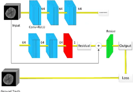
The proposed CNN model with 8 successive convolutional blocks were implemented by TensorFlow (Version 1.10). Each convolutional block consists of two 3-D convolutional layer followed by ReLU activation layers. The first 7 blocks in blue have 64-channel feature maps while the last block in red has 1-channel output, as shown in Fig. 1. A convolution based plain network has connections only between adjacent layers, as shown in Fig. 2(a). It will increase the training difficulty when the network becomes deeper due to gradient diffusion. In ResNet, a simple identity mapping directly connecting the input and output layers and bypass connection are added into the network [9, 22]. In the end, the 7 blue blocks were implemented with network structure of Fig. 2(b) and the last red block were implemented as Fig. 2(c). For each convolutional layer, kernel size was set to 5*5*5, stride was set to 1 and padding zeros at the edges of each feature map to keep image size consistent. Original CTP images of 30 passes were treated as ground truth. The downsampled 15-pass CTP was input to CNN model to extract feature maps and finally feature maps were resized to 30 passes as restored CTP output. Here the resize operation is easily realized with a deconvolutional layer with stride (1,1,2).
Fig. 1 The structure of residual CNN model.
Learning the differences between input data and ground truth, which is commonly called residual, has faster convergence speed when training CNN [15, 23]. This is because it is difficult to map the downsampled image data to ground truth with conventional CNN structure (eg. AlexNet and VGG) directly, since CNNs are usually initialized with small weights which will result in a large loss between the CNN output and ground truth to optimize. However, the residuals, which can be considered as the noise in input data, are much closer to 0 and easier to learn since CNN is initiated with an initializer of
Fig. 2 Plain network and residual network: (a) plain network, and (b) residual network, (c) revised residual network.
truncated normal distribution, where mean and standard deviation are 0.0 and 1.0 respectively. The proposed residual CNN model can be expressed by eq. 1,
( )
O(x)resize f(x)+ x (eq.1) where x is the input, f(x) is convolutional operations and O(x) is output.
In our task, the input data was divided into smaller patches of size 32*32*15. According to our computation, the receptive field of the 15 successive 5*5*5 convolutional layers is 61, which is large enough to cover the input image. When computing pixel-wise loss, the loss of each pixel was taken into account, which contributed to increasing training data volume significantly. Pixel-wise mean absolute error (L1 loss) was adopted in our proposed model
II.B Data preparation and network training
In this study, the CTP images were collected from eight eligible slice locations of 24 acute stroke patients, as demonstrated in Fig. 3. The scan protocol is detailed as follows: tube voltage, 80 kV; tube current, 250mA; slice thickness, 5mm. Each slice location has 30 CTP images with 512*512 pixels corresponding to 30 pass in time sequence. 18 of 24 patients were randomly selected as training set and the other 6 patients were used as test set. The original 512*512*30 data volume for each slice location was first downsampled to the dataset of size 512*512*15 to simulate reducing 15 scans. We subdivided the data volume to 32*32*N (N is 15 for training and 30 for test) 3-D patches along width and height directions as the input of CNN network, since batch size needs to be set higher when training the network with small patches [24]. Cropping stride was set to 16 and 32 for training and test dataset respectively.
The proposed CNN model was trained by adaptive moment estimation (Adam) optimization [25]. The initiated learning rate was set to 1e-4 and then decayed in each epoch. The batch size was set to 32. It took about 35 hours to train 10 epochs to acquire stable convergence on our PC (Core i5 CPU, 1080Ti GPU, 16G RAM), of which the loss would not decline.
III. Result Analysis
III.A Restoration results
After training, the test dataset was input into the trained CNN model. Original 30-pass CTP images were used as ground truth for verifying the validity of our interpolation CNN model. We also used cubic interpolation and deep convolutional GAN (DCGAN) to restore 15-pass CTP images for comparison. Cubic interpolation is a conventional interpolation method and easy to realize. DCGAN is a proven effective generative model for feature representation, image generation and image analysis [26]. Besides, 30-pass CTP images were also downsampled to 10 passes and then processed using the retrained CNN of proposed structure.
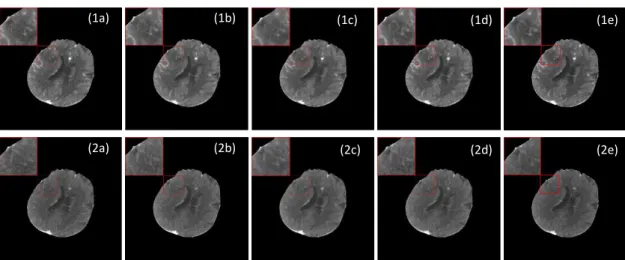
Fig.4 shows the 12th-pass and 18th-pass ground truth CTP images and restored downsampled images
of one selected patient using different algorithms from test dataset. The concentration of contrast agents, which is near the peak at 12th pass, decreases a lot at 18th pass in a brain blood circulation period. The
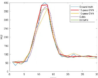
enlarged images of red box are shown in the top-left corner. From Fig.4, it can be seen that 15-pass CNN method can obtain high-quality CTP images with finer image details and clearer image edges, especially vascular details which is critical to calculate perfusion parameters. However, results of 10-pass CNN (c) are a bit fuzzy and lose some highlighted vessel pixels. Results of DCGAN (e) still exist some noise since that training of GAN is not stable [27]. Fig.5 gives the 30-pass time density curve (TDC) of anterior cerebral artery from the selected patient. From Fig.5, we can notice that curves generated by our 15-pass CNN is the closest to the ground truth, especially when the contrast density is high-level from the 10th
pass to 15th pass. Curve of 10-pass CNN (yellow) loses a lot of information during 10th and 15th pass.
Curve of cubic (purple) and DCGAN (green) show lower peak values and delay of reaching peak in time sequence. That will lead to higher TTP value when calculating perfusion parameters.
Fig. 4 The first row and second row are the 12th pass and 18th pass images of selected patient at slice
location 64. (a) is the original image, (b) is result of our 15-pass CNN, (c) is result of 10-pass CNN, (d) is result of 15-pass cubic interpolation, (e) is result of 15-pass DCGAN.
(1a) (1b) (1c) (1d) (1e)
Fig. 5 The time density curves of anterior cerebral artery from selected patient.
III.B Quantitative analysis
We evaluated the restored image quality quantitatively with structural similarity index (SSIM) and peak signal-to-noise ratio (PSNR). Definition of SSIM is demonstrated in eq. 2,
2 2 2 2 2 2 (2 )(2 ) ( , ) ( )( ) x y 1 xy x y 1 x y c c SSIM x y c c (eq.2)
where x andyare two images of same size,
and are average and covariance, c1k1*Land 2 2*c k Lare two variables to stabilize the division with weak denominator, k10.01,k20.03 by default, and
L
is the dynamic range of the pixel-values. SSIM ranges from 0 to 1, and 1 means the highest similarity. PSNR is defined as eq.3,10 10
( ) 20*log (MAX ) 10*log (MSE)I
PSNR x,y (eq.3) where MSE is mean square error between ground truth and the restored, MAXIis maximum pixel value of image.
Table 1 gives the average SSIM and PSNR of six test patients, each patient has eight slice location data. The global image means we calculated SSIM and PSNR with the whole restoration images of size 512x512. Although these four methods can restore the downsampled CTP effectively, with SSIM all over 0.97and PSNR over 50, the 15-pass CNN model acquire the highest SSIM and PSNR, which explains the best performance on restoring downsampled CTP images. Besides, our radiologists also selected regions of interest (ROI) of size 80x80 from the hypoperfusion areas to calculate mean ROI SSIM and PSNR. Results are given in Table 1 too. Among these four methods, the 10-pass CNN shows the lowest SSIM and PSNR, illustrating that it is hard to restore CTP images if omitting too many passes.
Table 1 The SSIM and PSNR of global images and ROI using different methods (Mean ± SD)
Global Image ROI
Methods SSIM PSNR SSIM PSNR
15-pass CNN 0.981 ± 0.0008 56.25 ± 1.77 0.915 ± 0.109 42.44 ± 8.51 10-pass CNN 0.973 ± 0.0011 54.84 ± 1.81 0.881 ± 0.155 40.94 ± 8.52
Cubic 0.976 ± 0.0010 55.29 ± 1.89 0.896 ± 0.134 41.39 ± 8.48
DCGAN 0.974 ± 0.0008 56.01 ± 1.73 0.910 ± 0.114 42.11 ± 8.52
III.C Perfusion parameters results
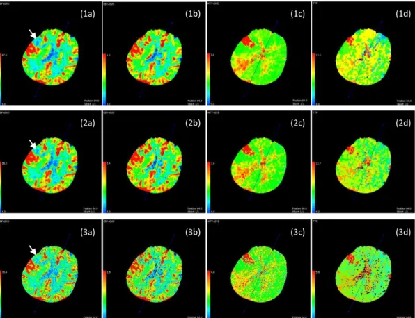
For acute stroke diagnosis and treatment, we care much about perfusion parameter maps. After restoring downsampled CTP images with CNN, we input the restored CTP to calculate perfusion maps with PMA software. Fig. 6 gives the CBF, CBV, MTT, TTP maps of the selected patient at slice location
Fig. 6 Perfusion maps of the selected patient. Three rows are maps calculated from ground truth CTP, 15-pass CNN restored results, and unprocessed 15-pass CTP respectively. (a) is CBF, (b) is CBV, (c) is
MTT, (d) is TTP.
64. Then two radiologists of our group reviewed the perfusion maps of different methods together and gave conclusions by consensus. According to Fig. 6, the restored CTP calculated perfusion maps share high similarity with ground truth CTP calculated maps. Both the first two rows indicate CBF descending, CBV ascending, MTT ascending, TTP ascending in right temporal lobe. In the third row, we gave the perfusion maps of unprocessed 15-pass images. In fact, the maps show imaging quality of unprocessed 15-pass images is worse than restored CTP images, which contain more scattered points. As indicated by the white arrows, perfusion maps of unprocessed images cannot reveal CBF severely degraded areas. Besides, the perfusion value ranges of unprocessed images greatly differs from that of ground truth. The maps of the third row are misleading for radiologists’ diagnosis. Hence, restoration is essential to improve the quality of perfusion parameter imaging.
We tested 6 patients’ restored CTP images of test dataset, and radiologists can get the same diagnostic conclusions and assessment as original ground truth CTP maps. Although the other three methods (10-pass CNN, cubic interpolation, DCGAN) could show the similar hypoperfusion areas to ground truth, they would lead to the considerable errors because of larger TTP and smaller CBF, CBV, MTT values. This would mislead radiologists’ diagnosis such as changed hypoperfusion area and inaccurate hypoperfusion level of test patients. Take the MTT map for example, Fig. 7 gives five maps of ground truth and the results of different algorithms. It is clear to see that the result of our 15-pass CNN is the closest to ground truth and has the consistent MTT range ([0, 7.6]), while maps of the other three methods have a lot of scattered points and larger MTT range (10-pass CNN: [0, 7.8], cubic: [0, 8.0], DCGAN: [0, 8.2]). It suggests that the 15-pass CNN can attain finer CTP image details and less artifacts which was stated in Section III.A. Table 2 presents the average perfusion values of four methods. Table
(1a) (1b) (1c) (1d)
(2a) (2b) (2c) (2d)
3 gives the root mean square error (RMSE) and mean absolute percentage error (MAPE) between different method results and ground truth of six test patients’ data. From Table 2 and Table 3, we can see that the parameter values of our 15-pass CNN are closest to the parameters values calculated from ground truth although they have small errors. In comparison, results of the other three methods have larger errors. Considering both RMSE and MAPE, our 15-pass CNN outperforms other three methods. Meanwhile, DCGAN has the least CBF error, displaying the restoration potential of generative model.
Table 2 The perfusion parameters using different algorithms of selected patient (Mean ± SD)
Ground Truth 15-pass CNN 10-pass CNN Cubic DCGAN
CBF 35.08±6.95 34.50±5.16 33.59±6.73 33.98±6.64 33.59±6.76
CBV 2.41±0.46 2.39±0.42 2.21±0.33 2.28±0.46 2.27±0.49
MTT 4.32±0.55 4.33±0.34 4.22±0.38 4.22±0.51 4.27±0.57
TTP 8.71±0.37 8.76±0.11 9.26±0.46 9.24±0.11 9.25±0.12
Table 3 The RMSE and MAPE of perfusion parameters using different algorithms
RMSE MAPE
15-pass CNN
10-pass CNN
Cubic DCGAN 15-pass CNN 10-pass CNN Cubic DCGAN CBF 3.245 3.208 2.674 2.531 6.73% 7.66% 6.12% 5.70% CBV 0.121 0.280 0.185 0.188 4.44% 8.76% 5.73% 6.53% MTT 1.653 3.321 1.801 1.759 4.58% 8.25% 3.39% 3.09% TTP 2.399 5.806 2.897 2.908 3.49% 8.61% 5.40% 5.45%
III.D Model efficiency analysis
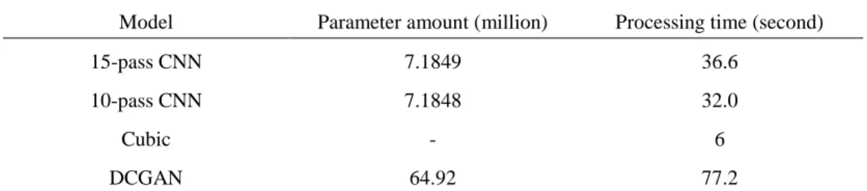
Table 4 The parameter amount and mean processing time of different models
Model Parameter amount (million) Processing time (second)
15-pass CNN 7.1849 36.6
10-pass CNN 7.1848 32.0
Cubic - 6
DCGAN 64.92 77.2
In this section, we mainly discuss the model running speed and memory use. For deep neural networks, the model parameter amount is most concerned. In this study, the parameter amount of 15-pass CNN is about 7.1849 million, while 10-15-pass CNN is 7.1848 million and DCGAN is 64.92 million. The massive parameters contained in DCGAN make it hard to train. Due to the same topological structures of 15-pass CNN and 10-pass CNN, their parameter amounts are almost same. The parameter amounts of classical VGG-16 [28] and ResNet-50 [9] are 138 million and 25 million, so our 15-pass CNN is much simpler by contrast. After training the CNN model, it took about 220 seconds to generate all six patients’ restoration CTP images. The mean time for each patient is 36.6s, which is fast enough
Fig. 7 MTT maps of the selected patient calculated from different results. (a) is ground truth, (b) is results from 15-pass CNN, (c) is 10-pass CNN, (d) is cubic interpolation, (e) is DCGAN
for imaging since that running on a PC with Core i5 CPU. However, running time for each patient with DCGAN is over 77s because of too many parameters. Cubic interpolation has the fastest speed, with processing time of 6s each, as shown in Table4, but has low imaging quality.
IV. Discussion
Perfusion imaging is a common method for acute stroke examination. It usually takes about 50s for blood to circulate the whole body. Most imaging workstations, like GE and Philips, scan brain 30 times within 50s after injecting contrast agents consequently. The 30-pass CTP scan will significantly increase the radiation dose. Hence, it inspires us to reduce the scan frequency. We first downsampled the original CTP to 15 passes to reduce a half radiation dose. However if we calculated with the scan-reduced CTP images directly, the perfusion parameter value would be inaccurate as illustrated in Fig.6. Then we used a trained CNN model to restore 15-pass CTP images to 30-pass images for calculating perfusion maps. Residual learning is necessary in this task. In our experiments, if we did not add the residual skip connection in CNN structure, the L1-loss value would be very large during the first several training iterations. However, in residual structure, the CNN just needs to learn the difference between downsampled CTP and ground truth. It will accelerate the convergence speed of deep neural networks. According to our experiments, the loss can decline quickly with residual skip connection. It only needs less than 200 iterations to bring down loss below 1 with initial learning rate of 1e-4. In comparison, the loss would descend slowly and fluctuate if without residual skip connection. At last, we just trained our CNN model 10 epochs efficiently. Residual learning has shown its excellent performance in the restoration CNN.
After restoring 30-pass CTP images from downsampled 15-pass CTP, perfusion parameters can be computed. However, different perfusion tools will acquire different results, even from identical source data [29, 30]. Some softwares may overestimate or underestimate ischemic core. This is probably because of differences in tracer delay sensitivity and postprocessing algorithms. The common perfusion postprocessing algorithms can be classified into three categories: Gamma Fitting, Maximum Slope and Deconvolution. Kudo et al. [31] assessed the accuracy and reliability using a digital phantom with 13 perfusion postprocessing algorithms. Experiment results illustrate that the single value decomposition (SVD) of PMA can achieve the closest CBF, CBV and MTT values to ground truth. Hence, PMA was employed to calculate CBF and other perfusion maps in this study. We calculated the mean perfusion values from 15-pass CNN, 10-pass CNN, cubic interpolation and DCGAN output using PMA. And the errors prove that 15-pass CNN has the best results.
V. Conclusion
In this work, we proposed an optional way to reduce CTP imaging radiation dose, that is downsampling 30-pass images to 15 passes in temporal domain and then restoring them to 30 passes with the deep residual CNN model. Finally, with the help of the radiologists of the First Hospital of Jilin University in China, we can find out the coincident hypoperfusion areas according to perfusion parameters calculated from restored CTP and original CTP. Experiment results have presented its effectiveness. Moreover, the post-processing time is also within acceptable limits. In the future, we will focus on reducing radiation dose not only in time sequence, but also in spatial domain [32]. How to cut down the CTP scan frequency and reduce the imaging tube current at the same time and then process with a CNN model to recover high-quality CTP images is our next research program.
10
Funding
This work was supported in part by the State’s Key Project of Research and Development Plan under Grant 2017YFA0104302, Grant 2017YFC0109202 and 2017YFC0107900, National Natural Science Foundation under Grant 81530060, 31571001 and 81471752, and the R&D Projects in Key Technology Areas of Guangdong Province under Grant 2018B030333001.Compliance with ethical standards
Conflict of Interest The authors declare that they have no conflict of interest.
Ethical approval All procedures performed in studies involving human participants were in accordance with the ethical standards of the institutional and/or national research committee and with the 1964 Helsinki declaration and its later amendments or comparable ethical standards.
Informed consent Informed consent was obtained from all individual participants included in the study.
References
1. Wang L, Wang J, Peng B (2016) China stroke prevention report 2016 summary. Chinese Journal of Cerebrovascular Diseases 14:217-224
2. Chinese Medical Association Cerebrovascular Disease Group (2018) Guidelines for the diagnosis and treatment of acute ischemic stroke in China. Chinese Journal of Neurology 51: 666-682
3. Krishnamoorthi R, Ramarajan N, Wang N E, Newman B, Rubesova E, Mueller C M, Barth R A (2011) Effectiveness of a staged US and CT protocol for the diagnosis of pediatric appendicitis: reducing radiation exposure in the age of ALARA. Radiology 259: 231-239
4. Liu J, Hu Y, Yang J, Chen Y, Shu H, Luo L, Feng Q, Gui Z, Coatrieux G (2018) 3D Feature Constrained Reconstruction for Low Dose CT Imaging. IEEE Transactions on Circuits and Systems for Video Technology 28:1232-1247
5. Bian J, Wang J, Han X, Sidky E Y, Shao L, Pan X (2013). Optimization-based image reconstruction from sparse-view data in offset-detector CBCT. Physics in Medicine & Biology 58: 205
6. Cho S, Pearson E, Pelizzari C A, Pan X (2009) Region-of-interest image reconstruction with intensity weighting in circular cone-beam CT for image-guided radiation therapy. Medical physics 36: 1184-1192 7. Kalke M, Siltanen S (2014) Sinogram interpolation method for sparse-angle tomography. Applied
Mathematics 5: 423.
8. Zhang H, Sonke J J (2013) Directional sinogram interpolation for sparse angular acquisition in cone-beam computed tomography. Journal of X-ray science and technology 21: 481-496
9. He K, Zhang X, Ren S, Sun J (2016) Deep residual learning for image recognition. Proceedings of the IEEE conference on computer vision and pattern recognition 770-778
10. Chen L C, Papandreou G, Kokkinos I, Murphy K, Yuille A L (2018) Deeplab: Semantic image segmentation with deep convolutional nets, atrous convolution, and fully connected crfs. IEEE transactions on pattern analysis and machine intelligence 40: 834-848.
11. Ronneberger O, Fischer P, Brox T (2015) U-net: Convolutional networks for biomedical image segmentation. International Conference on Medical image computing and computer-assisted intervention. 234-241 12. Dong C, Loy C C, He K, Tang X (2016) Image super-resolution using deep convolutional networks. IEEE
transactions on pattern analysis and machine intelligence 38: 295-307.
13. Chen H, Zhang Y, Chen Y, Zhang J, Zhang W, Sun H, Lv Y, Liao P, Zhou J, Wang G (2018) LEARN: Learned experts’ assessment-based reconstruction network for sparse-data CT. IEEE transactions on medical imaging 37:1333-1347.
14. Lee D, Choi S, Kim H J. (2018) High quality imaging from sparsely sampled computed tomography data with deep learning and wavelet transform in various domains. Medical physics 46: 104-115
11
15. Lee H, Lee J, Cho S. (2017) View-interpolation of sparsely sampled sinogram using convolutional neural network. Medical Imaging 2017: Image Processing. International Society for Optics and Photonics. https://doi.org/10.1117/12.2254244
16. Wolterink J M, Leiner T, Viergever M A, Ivana I. (2017) Generative adversarial networks for noise reduction in low-dose CT. IEEE transactions on medical imaging 36: 2536-2545.
17. Kudo K, Sasaki M, Yamada K, Momoshima S, Utsunomiya H, Shirato H, Ogasawara K (2009) Differences in CT perfusion maps generated by different commercial software: quantitative analysis by using identical source data of acute stroke patients. Radiology 254: 200-209
18. Wang G. (2016) A Perspective on Deep Imaging. IEEE Access 4:8914 – 8924
19. Long J, Shelhamer E, Darrell T (2015) Fully convolutional networks for semantic segmentation. Proceedings of the IEEE conference on computer vision and pattern recognition 2015: 3431-3440
20. Krizhevsky A, Sutskever I, Hinton G E (2012) Imagenet classification with deep convolutional neural networks. Advances in neural information processing systems. 2012: 1097-1105.
21. Petneházi G. (2019) Recurrent neural networks for time series forecasting. arXiv preprint arXiv:1901.00069. 22. Chen H, Zhang Y, Kalra M K, Feng L, Yang C, Peixi L, Jiliu Z, Ge W. (2017) Low-dose CT with a residual
encoder-decoder convolutional neural network. IEEE transactions on medical imaging 36: 2524-2535. 23. Yang W, Zhang H, Yang J, Wu J, Yin X, Chen Y, Shu H, Luo L, Coatrieux G, Gui Z, Feng Q (2017) Improving
low-dose ct image using residual convolutional network. IEEE Access 5: 24698-24705
24. Yin X, Zhao Q, Liu J, Yang W, Yang J, Quan G, Chen Y, Shu HZ, Luo LL, Coatrieux JL. (2019) Domain Progressive 3D Residual Convolution Network to Improve Low Dose CT Imaging. IEEE, Transactions on Medical Imaging, doi: 10.1109/TMI.2019.2917258
25. Kingma D P, Ba J. (2014) Adam: A method for stochastic optimization. arXiv preprint arXiv:1412.6980 26. Radford, A., Metz, L., & Chintala, S. (2016) Unsupervised Representation Learning with Deep Convolutional
Generative Adversarial Networks. International Conference on Learning Representations (ICLR).
27. Gulrajani I, Ahmed F, Arjovsky M, Dumoulin V, Courvile A. (2017) Improved training of wasserstein gans. Advances in neural information processing systems (NIPS).
28. Karen S., Andrew Z. (2015) Very deep convolutional networks for large-scale image recognition. International Conference on Learning Representations (ICLR).
29. Kudo K, Sasaki M, Yamada K, Momoshima S, Utsunomiya H, Shirato H, Ogasawara K. (2009) Differences in CT perfusion maps generated by different commercial software: quantitative analysis by using identical source data of acute stroke patients. Radiology, 254: 200-209.
30. Austein F, Riedel C, Kerby T, Meyne J, Binder A, Lindner T, Huhndorf M, Wodarg F, Jansen O. (2016) Comparison of perfusion CT software to predict the final infarct volume after thrombectomy. Stroke, 47: 2311-2317.
31. Kudo K, Christensen S, Sasaki M, Ostergaard L, Shirato H, Wintermark M, Warach S. (2013) Accuracy and reliability assessment of CT and MR perfusion analysis software using a digital phantom. Radiology, 267: 201-211.
32. Liu J, Ma J, Zhang Y, Chen Y, Yang J, Shu H, Luo L, Coatrieux G. (2017) Discriminative feature representation to improve projection data inconsistency for low dose CT imaging. IEEE transactions on medical imaging, 36: 2499-2509.