Complete analytical procedure to assess the response of a frame submitted to a column loss

1

Complete analytical procedure to assess the response of a frame

submitted to a column loss

Clara Huvelle, Van-Long Hoang, Jean-Pierre Jaspart, Jean-François Demonceau University of Liège

Corresponding author:

Jean-François Demonceau, Chemin des Chevreuils, 1 B52/3, 4000 Liège - Belgium Phone: +3243669358 - e-mail : jfdemonceau@ulg.ac.be

Abstract

The present paper gives a global overview on recent developments performed at the University of Liege on structural robustness of buildings for the specific scenario “loss of a column”. In particular, a complete analytical method to assess the response of a 2D frame losing statically one of its columns is presented in details. This method is based on the development of alternative load paths in the damaged structure and takes into account the couplings between the different parts of the structure which are differently affected by the column loss. Also, the validation of the developed method through comparison to experimental and numerical evidences is presented.

Keywords: robustness, column loss, analytical model, steel structures, building structures, exceptional event

1

Introduction

Recent events such as natural catastrophes or terrorism attacks have highlighted the necessity to ensure the structural integrity of buildings under an exceptional event. According to Eurocodes and some other national design codes, the structural integrity of civil engineering structures should be guaranteed through appropriate measures and one way to guarantee it is to ensure an appropriate robustness of the structure, which may be defined as the ability of a structure to remain globally stable in case of exceptional event leading to local damages. However, although global design approaches such as the activation of alternative load paths or the key element method are provided in modern codes and standards, no easy-to-apply practical guidelines are provided. The present

2 paper reflects recent researches realised at the University of Liege with the objective of proposing such practical guidelines for the activation of alternative load paths in the structure, knowing that this design strategy generally leads to the most economical solutions.

2

Background

The behaviour of steel and composite frames under the exceptional event “loss of a column” have been recently investigated through many researches (e.g. from [1] to [13] among others).

At the University of Liege, this topic is under investigation since many years using experimental, numerical and analytical approaches [2]. The adopted general philosophy in Liege is to observe the redistribution of the loads in damaged structures through the activation of alternative load paths and to develop analytical methods to predict this redistribution of loads. Knowing how the loads are redistributed, it is possible to estimate whether or not the remaining elements are able to sustain the additional loads coming from this redistribution, without causing a progressive collapse of the entire frame.

Two PhD theses have already been finalised on these topics in Liege (Demonceau [4] and Luu [11]). These theses have contributed to the development of a first analytical method that allows predicting the response of frames submitted to a column loss, and in particular, the associated catenary actions. This initial method has been recently improved and completed. The present paper gives a precise description of this improved analytical procedure.

2.1 General philosophy

When a frame is submitted to a column loss, two parts can be identified in the structure: the directly affected part and the indirectly affected part. The directly affected part contains all the beams, columns and beam-to-column joints located just above the lost column (Figure 1). The rest of the structure (i.e. the lateral parts and the storeys under the lost column) is defined as the indirectly affected part.

When the frame loses one of its columns (column AB in Figure 1a), the evolution of the compression force NAB in this element VS the vertical displacement (u) at the top of this column is divided in 3

3 phases as illustrated in Figure 1. During phase 1 (from (1) to (2) in Figure 1b), i.e. before the event, the column is “normally” loaded (i.e. the column supports the loads coming from the upper storeys) and the corresponding load is named NABnormal.

a) Frame description b) Behaviour description Figure 1. Behaviour of a frame submitted to a column loss

Phase 2 (from (2) to (4) in Figure 1b) begins when the event occurs and the column progressively loses its axial resistance. During this phase, a plastic mechanism develops in the directly affected part. Each change of slope in the curve of Figure 1b corresponds to the development of a new hinge in the directly affected part, until reaching a complete plastic mechanism (point (4) in Figure 1b). Phase 3 (from (4) to (5) in Figure 1b) starts when this plastic mechanism is formed: the vertical displacement at the top of the lost column increases significantly since there is no more first order rigidity in the structure. As a result of these large displacements, catenary actions develop

progressively in the beams of the directly affected part, so providing a second-order stiffness to the structure. The role of the indirectly affected part during phase 3 is to provide a lateral anchorage to these catenary actions: the stiffer the indirectly affected part is, the higher the catenary actions will be in the directly affected part. In the extreme situation where the indirectly affected part has no lateral stiffness, then no catenary actions will develop and phase 3 will not develop.

4 The behaviour of the actual structure from (2) to (5) (Figure 1b) may be predicted simulating the behaviour of the structure as shown in Figure 2; the frame without the lost column AB is subjected to a concentrated load P going downward and applied at node A.

The objective with the analytical method developed in Liege is to determine a P-u curve reflecting the behaviour of the simulated structure, to estimate the redistribution of loads within the structure during these phases and finally to check whether the structure is able or not to reach point (5), i.e. when P = NABnormal. Indeed, this point is reached only if there is enough resistance and ductility in the

damaged structure to sustain these large displacements and associated forces coming from the activation of alternative load paths.

The analytical model presented herein focuses on the behaviour of the frame during Phase 3 (from (4) to (5)), the behaviour of the frame during Phase 2 being easily predicted through classical approaches.

Figure 2. Simulation of the column loss

2.2 Demonceau model

In Demonceau thesis [4], an analytical method has been developed that allows predicting the P-u curve during phase 3 (Figure 1) for the case of a 2D structure losing statically one column. The method is focusing on phase 3, i.e. when second order effects are predominant, and is based on the study of a substructure that contains only the lower beams of the directly affected part (Figure 3), identified as the beam where higher tension forces appear. The surrounding structure is simulated by a horizontal spring with a stiffness KH (Figure 3). This KH has a constant value in the model as it is

5 assumed that the indirectly affected part remains elastic during phase 3. Of course, this constitutes a simplification of the actual behaviour of the indirectly affected part as the latter can yield during this phase; the revision of this assumption will be considered in the future developments.

Figure 3. Substructure considered in the Demonceau model [4] The input data of this method are the following:

- L0: initial length of the beam (Figure 3).

- M-N resistance interaction curve for both hogging and sagging bending in the plastic hinges (located in a beam cross-section or in a joint). These laws can be determined by [14] or [15] for joints and [16] or [17] for beam cross-sections.

- KH: stiffness of the horizontal spring (Figure 3).

- KN: axial stiffness of a plastic hinge submitted to both bending and axial forces (defined as the ratio

between the axial force N and the plastic elongation of the hinge δN - see Figure 3).

During phase 2, the hinges are only submitted to bending (A-B on Figure 4) while, during phase 3, they are submitted to both M and N (B-C on Figure 4). At the very end of phase 3, they could possibly even only be submitted to N (point C on Figure 4). The relation between N and δN is assumed to be

linear and totally defined by this parameter KN (Figure 4). This assumption has been validated

6 Figure 4. Behaviour of the yielded sections

The unknowns and equations obtained from the study of the substructure given in Figure 3 are reported in Table 1. As the number of equations is equal to the number of unknowns, this system can be easily solved for different values of u.

In [4], it is demonstrated that this substructure model is able to reflect accurately the response of a frame further to a column loss if the parameters KN and KH are appropriately estimated.

As the substructure defined by Demonceau takes into account only one storey of the frame that suffers the column loss, the parameter KH should reflect the behaviour of all the structure around,

i.e. on the one hand, the storeys of the directly affected part above the lost column, and on the other hand, the indirectly affected part located beside.

Table 1. Unknowns and equations of the Demonceau model Unknowns Equations u u = input data θ sin(θ)= u/( L0+2 δN) δh cos(θ)= ( L0- δH/2)/( L0+2 δN) δN δH = FH/KH P δN = N/KN N M = f(N) ([1] or [17]) M -0.25P(L0-0.5δH)+0.5FHu+2M=0 Fh N = FHcos(θ)+0.5P sin(θ)

However, no analytical procedure was proposed in [4] for this parameter KH. Also, the parameter KN

was numerically or experimentally estimated for the validation of Demonceau model in [4], but no analytical prediction model was suggested.

N M M N δN θ A A A=B B B C C C O-A = Phase 1 A-B = Phase 2 B-C = Phase 3 KN O

7 Therefore, to have a complete analytical procedure, it was necessary to develop analytical models to predict the values of both KN and KH parameters. This task has been achieved; it is presented in

paragraphs 3 and 4 respectively.

3

Local parameter: K

The KN parameter is defined as a local parameter, because it is linked to the behaviour of the yield

zones in the directly affected part. These yield zones can occur in the beam cross-section or in the beam-to-column joint if partial strength joints are used. The developed analytical method is presented for both cases. In this paragraph, the KH is assumed to be an input data and only

one-storey substructure (as defined previously) is studied.

3.1 Hinge forming in the beam cross-section

3.1.1 Parametrical study

A range of numerical tests has been performed on the one-storey structure presented in Figure 5. For sake of simplicity, the structure is assumed symmetrical. These simulations have been performed using the homemade software Finelg [18], developed at the University of Liege, taking into account the material and geometric non linearity. The aim was to understand whether the KN was a

cross-section characteristic, or if there was a coupling between the hinge behaviour and the global structure in which this hinge was developing.

Figure 5. Investigated one-storey substructure to study the plastic elongation of the yield zones The value of δN was extracted from the numerical results u and δH as follows:

=1_{2 − +} ² + − P KH δH L0 u L0+2δN 2D analysis L0 = 7 m IPE550

8 Although it has been shown by other parametrical studies that the value of KN depends on the value

of E, fy, and on the cross-section geometrical properties, it appeared that the main parameter

influencing the value of KN was the parameter KH (Figure 6). So, it can be concluded that, in addition

to the dependence of KN on the cross section characteristic, it also depends globally on the structure

in which the hinge develops.

Figure 6. N vs. δN curves for different values of KH

3.1.2 New approach

To define an analytical model for the prediction of KN, it is required to define a length for the plastic

hinge. This hinge length L is defined according to [19] (see Figure 7).

Figure 7. Plastic hinge length definition [19]

Then, the cross-section is fictively divided into 6 parts: 2 parts represent the flanges and 4 parts the web (Figure 8). Finally, the extremities of the beams of the directly affected part can be considered

0 1000 2000 3000 4000 5000 0 0,02 0,04 0,06 0,08

N

[

k

N

]

δ

9 as a set of 6 parallel springs submitted to M and N, assuming that the section at the extremities of these springs remains straight, using the Bernoulli assumption (Figure 8).

Figure 8. Spring model for the beam cross-section

The force-displacement law of each spring is elastic-perfectly plastic and symmetric in tension and in compression. The resistance of each spring is simply equal to Frdi = Aify and the stiffness Ki = EAi/L,

where L is the length of the considered hinge, Ai represents the section of part “i” and E the Young

modulus of the beam material.

When reaching point B on the M-N diagram (Figure 9, beginning of phase 3), all the springs are yielded (as a hinge is formed in the considered cross-section) and the springs 3 and 4 on Figure 9 have just reached their maximum elastic elongation, Frd/K, so δ and θ are known at point B. When

going from B to B1, the spring n°4 is “unloading” from –Frd to Frd, and so remains in the elastic range.

During this time, all the other springs are still in the plastic domain, so there is no information on their elongation. Finally at point B1, neither δ nor θ can be defined as there are two unknowns (δ and θ) and only one piece of information (the elongation of spring n°4). In other words, no relation between δ and θ may be found locally. In fact, the missing equation between δ and θ comes from the analysis of the global structure in which the hinge forms, so explaining why KN depends on KH.

10 Figure 9. Response of the spring model under M and N

As there is a coupling between this local parameter KN and the global structural response in which

the hinge is developing, the local hinge model has to be implemented in the substructure of Demonceau (Figure 10).

Figure 10. New substructure model The input data of this new substructure model are:

- The characteristics of the cross section (A, I, Wel, Wpl, dimensions...), also used for the definition of

the spring properties simulating the behaviour of the hinges - L0, E, fy, KH

11 There is no need any more to define a M-N resistance curve or to explicitly define KN linking N to δN,

because these data are implicitly included in the definition of the stiffness and resistances of the springs simulating the hinges at the extremities of the beam.

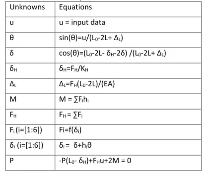
Table 2. Unknowns and equations for the new substructure model Unknowns Equations u u = input data θ sin(θ)=u/(L0-2L+ ΔL) δ cos(θ)=(L0-2L- δH-2δ) /(L0-2L+ ΔL) δH δH=FH/KH ΔL ΔL=FH(L0-2L)/(EA) M M = ∑Fihi FH FH = ∑Fi Fi (i=[1:6]) Fi=f(δi) δi (i=[1:6]) δi = δ+hiθ P -P(L0- δH)+FHu+2M = 0

The equations defined in Table 2 can easily be solved through a mathematical solver, for instance Matlab used for the presented study. Figure 11 shows a comparison between numerical and analytical results for different values of KH. The good agreement obtained between the results

validates the proposed approach.

Experimental tests on the deformability of plastic hinges under M-N interaction are planned at the University of Liege in 2014; they should confirm the numerical and analytical results.

3.2 Hinge forming in partial strength joints

If the beam-to-column joints are partially resistant, then the hinge develops in the joint and not in the beam cross-section. Nevertheless, the approach remains the same as previously described, except that the hinge length is assumed to be equal to 0. Indeed, the yield zone is localized in the joint, which is assumed to be very short compared to the length of the beam.

12 Figure 11. Comparison between numerical (continuous lines) and analytical (dash lines) results for

different values of KH

An experimental test has been conducted in Liège in 2008, within the European RFCS project Robustness ([3] and [20]). The test was simulating the static loss of the central support of a composite beam (Figure 12). Horizontal jacks were placed at the extremities of the specimen to simulate the horizontal restraint of the indirectly affected part. More details about this test can be found in [3] (and also in [4]).

At the time of the test, the analytical determination of KN was not available, so the value of KN that

had to be introduced in the Demonceau model had been extracted from experimental tests conducted on the joints in isolation at the University of Stuttgart within the same European project Robustness [20].

According to the latest developments in Liege, it is now possible to determine this curve without any experimental or numerical input, as shown hereunder.

0 500 1000 1500 2000 2500 -3,5 -3 -2,5 -2 -1,5 -1 -0,5 0

P

[

k

N

]

δ

13 Figure 12. Substructure test conducted at the University of Liege

As for the cross-section, the joint is simulated by springs in parallel. The force-elongation relationship of these springs are elastic perfectly plastic. No limitation in the ductility of the components is assumed for the moment. One spring per joint row is defined, and the characteristics of the spring (stiffness K and resistance F) are determined through the component method, which is

recommended in Eurocode 3 and Eurocode 4 for the characterisation of joint properties ([21] and [22]). For the specific joints used for the Liège test, 11 joint rows are identified (Figure 13). For the concrete components (Rows 1, 3, 5 and 7 – see Figure 13), the stiffness is defined according to the formulae developed by Demonceau in [4] (see also [15]) as no rules are presently available for the characterisation of this component in Eurocode 4.

Another difference with the model used for the beam cross-section is that the behaviour of the springs is not symmetric in tension and in compression (Figure 14). For example, the bolts are only activated in tension, while the beam flange is only active in compression as considered in the

component method. Also, during the loading, some components could be inactive in the beginning of the loading, under M only (phase 2), and be activated when catenary action develops (phase 3) and conversely. So, it is necessary to define the way these components behave actually. For example, let assume that, during phase 2, a bolt row is submitted to a negative displacement (meaning that the bolt is in compression). The displacement goes from A to B in Figure 14, without forces in the bolt

14 row. At the point B, the displacement at the bolt level starts to increase. To be activated, the

displacement must return to 0, and then, the bolt can develop tension forces (Figure 14). Accordingly, for each load step, the loading history in each row has to be known.

Figure 13. Steel-concrete composite joint configuration of the Liege test

Figure 14. Behaviour law of a joint raw

The input data to be used in the analytical model for the experimental test previously described are: - L0 = 4 m 500 A B C F Δ

15 - KH = 8560 kN/m

- Spring characteristics for the joint: hi Fi Ki, given in Table 3, “i” being the number of the joint row

under consideration (Figure 13)

Table 3. Properties of the joint row of the composite joint described in Figure 13

ROWS 1 2 3 4 5 6 7 8 9 10 11 h_{i [mm]} (*) _{146.5 127 116.5 106 95.5 85 65.5 42.6 11 -59 -90.6} Ki [103_kN/m] 2173.5 85.47 2173.5 85.47 2173.5 85.47 2173.5 1453.8 200.13 200.13 145.8 F_{i + [kN]} 0 66.35 0 66.35 0 66.35 0 0 224.22 91.55 0 F_{i – [kN] -340. 8} 0 -183.5 0 -183.5 0 -340.8 -374.8 0 0 -374.8 (*)_{: h}

i is the distance from row i (Figure 13) to the neutral axis (see Figure 9)

Solving the system of equations as given in Table 4, the response of the tested substructure can be analytically predicted. The results of the analytical method are compared with the experimental ones in Figure 15.

It can be seen that the analytical curve fits correctly with the experimental curve during phase 3, which is the phase under investigation. This validates the so-proposed model.

Figure 15. Comparison between the analytical prediction and the test result -40 -20 0 20 40 60 80 100 0 100 200 300 400 500 600 700 P [ k N ] u [mm] Experimental result Analytical result

16 Table 4. Unknowns and equations to be considered for the Liege test

Unknowns Equations

u u = input data

θ sin(θ)=u/L0

δSAG L0(cos(θ)-1)+ δH + δSAG + δHOG=0

δHOG FH = ∑FiSAG

FH FH = ∑FiHOG

δH δH=FH/KH

MHOG MHOG = ∑FiHOGhi

MSAG MSAG = ∑FiSAGhi

FiHOG (i=[1:11]) FiHOG=f(δiHOG)

FiSAG (i=[1:11]) FiSAG=f(δiSAG)

δiHOG (i=[1:11]) δiHOG = δHOG+hiθ

δiSAG (i=[1:11]) δiSAG = δSAG-hiθ

P P(L0cos(θ))(FHu+MHOG-MSAG)=0

4

Global parameter: K

In previous developments conducted in Liege (and in particular by Demonceau – Section 2.2), the substructure defined to study phase 3 was composed only of the lower beam of the directly affected part, i.e. the beams just above the lost column. The rest of the structure (i.e. the indirectly affected part) was only represented by one horizontal spring (see Figure 3).

However, this substructure is only valid if the compression force in the column just above the lost one remains constant during the all duration of phase 3, which is not always the case, as it has been demonstrated in [10] and [7]. Indeed, important coupling effects between the storeys of the directly affected part and also between the directly and the indirectly affected parts may develop and these effects should be considered into the developed model.

The coupling effects between the directly and the indirectly affected part could be taken into account through an appropriate definition of KH while, for the couplings between the storeys of the

17 Demonceau, i.e. a spring that could simulate the effect of the upper storeys of the directly affected part.

Accordingly, a general approach has been developed to take into account these coupling effects. A first method is presented in [8] without taking into account the effects of KN on these couplings. The

next paragraph will describe precisely the complete analytical method taking into account the effect of KN.

4.2 Complete analytical method

To consider all the couplings between the directly and indirectly affected parts, it is necessary to include all the storeys in the substructure model. So, the substructure defined by Demonceau is generalized for all the storeys of the directly affected part (Figure 16) and the effects of KN are added

to this generalized substructure by considering the extremities of the beams with springs in parallel. On the other hand, the influence of the indirectly affected part is taken into account by considering horizontal springs at each extremities of the so-defined substructure.

The springs simulating the restraint of the indirectly affected part are assumed as fully elastic as the indirectly affected part is assumed to be perfectly elastic (i.e. as assumed in Demonceau model – see Section 2.2).The horizontal displacement δHi at the storey i is defined as follows: δHi = ∑ sij FHj, in which

the coefficients sij form the flexibility matrix of the indirectly affected part (i.e. sij is the horizontal

displacement at the level i when a unitary horizontal force acts at the level j – see Figure 17) and FHj is

the horizontal load applied at storey j. In Figure 17, sl,ij sr,ij are respectively the displacements of the

18 Figure 16. Definition of a new substructure

Figure 17. Definition of the sij coefficients of the flexibility matrix

The input data for the final analytical model are given in Table 5. 1 kN Loads Displacements sl,12 sl,13 sl,11 sr,12 sr,13 sr,11 (a) sl,22 sl,23 sr,22 sr,23 sr,21 sl,2,1 1 kN (b)

19 The validation of the proposed model has been done through several comparisons between

numerical and analytical results for the frames shown in Figure 18. In these study cases, the beam-to-column joints are assumed to be full-strength and fully rigid. Finelg program [18] has been used for the numerical analysis. A good agreement is globally observed. A limited divergence of the curves can however be observed when significant membrane forces are developing. This can be explained through the following observation. In the analytical model, the length of the yielded zone is fixed from the beginning to the end of the curve (see Section 3.1.2) while, in the numerical model, the yielding can spread all along the beam. Accordingly, when significant plasticity is developing in the beams, a more flexible response is observed through the numerical model. However, it can be concluded that the analytical model is sufficiently accurate.

Table 5. Input data for the final analytical model characteristics of the cross section of the beams (A, I, Wel,

Wpl, dimensions, ...)

These parameters allow the computation of the following values: L, hi of the springs, Ai,

Frdi, Ki

L0

E, fy

nst = number of stories of the DAP

n = stories under the lost column

characteristics of the cross section of the columns c = number of columns in the IAP (right and left)

20 Beams: IPE550, S355, 7m of spans

Columns: HEB300, S355, 3.5m pf height

Load (vietcal, kN) – displacement (horizontal, m) curves (continuos lines: numerical; dash lines: analytical) Figure 18. Validation of the analytical model through comparisons to numerical results

0 1000 2000 3000 -2 -1,5 -1 -0,5 0 0 400 800 1200 1600 -2 -1,5 -1 -0,5 0 0 2000 4000 6000 -2,5 -2 -1,5 -1 -0,5 0

P

P

P

21 Table 6. Unknowns and equations for the final analytical model

Unknowns Number Equations Number

u 1 u = input data 1 θ nst sin(θ)=u/(L0-2L+ ΔL) nst δ nst cos(θ)=(L0-2L- δH-2δ) /(L0-2L+ ΔL) nst δH,l nst δH,l(nstx1)=Sl (nstnst)FH (nst) nst δH,r nst δH,r(nst1)=Sr (nstnst)FH (nst) nst ΔL nst ΔL=FH(L0-2L)/(EA) nst M nst M = ∑Fihi nst FH nst FH = ∑Fi nst Fi (i=[1:6]) 6* nst Fi=f(δi) 6* nst δi (i=[1:6]) 6* nst δi = δ+hiθ 6* nst P nst -0.5P(L0-0.5( δH,l+ δH,r))+FHu+2M = 0 nst Ptot 1 Ptot=∑P 1

5

Discussion and conclusion

The full analytical method presented in this paper allows predicting the response of a frame submitted to a column loss. It has been shown in the paper that the analytical results are in good agreement with numerical and experimental results, for simple substructure as well as for complete frames. The developed method takes into account the following phenomena:

- the global interaction between the different parts of the structure;

- the local phenomena occurring in the yield zones, submitted to both M and N.

The method presented here deals with 2D frames, submitted to a static column loss. Also, it is assumed that the indirectly affected part remains elastic and so the horizontal restraints brought by the indirectly affected part are constant during phase 3.

Other research works are now being conducted in Liege to deal with aspects such as the 3D

structural response, the possible dynamic effects associated to an impact or a blast loading and the progressive yielding of the indirectly affected part ([10], [1] and [7] respectively).

22 For the simulation of the joints, some simplifying assumptions have been made; for example, the group effects are not considered, the concrete in composite joints is assumed to have an infinite ductility and the shear interaction in the yield zones is neglected. These points are also being investigated further.

The final aim of these developments is to propose practical guidelines, design recommendations or easy-to-use software, founded on a good knowledge of the structural behaviour, and so to help practitioners facing robustness issues in design offices.

6

Table of notations

NAB Compression force in the column

NAB,normal Compression force in the column before it disappears

P Force simulating the loss of the column

u Vertical displacement at the top of the lost column

KH Stiffness of the horizontal spring simulating the lateral restraint of the indirectly

affected part

FH Horizontal force acting on the spring KH

δH Horizontal elongation of the spring KH

KN Axial stiffness of a plastic hinge submitted to bending and axial force

δN Axial elongation a plastic hinge submitted to bending and axial force

N Axial force in the beams of the directly affected part

M Bending moment at the extremities of the beams of the directly affected part θ Rotation at the extremities of the beams of the directly affected part

L0 Initial length of the beams

ΔL Elastic elongation of the beams of the directly affected part L Length of the plastic hinge (plasticized zones)

sij Displacement at the storey i for a force acting at the level j of the indirectly affected

part

23

7

References

[1] Comeliau L., Rossi B., Demonceau J.-F. Robustness of steel and composite buildings suffering the dynamic loss of a column. Structural Engineering International journal, Vol. 22/3, pp. 323-329, 2012.

[2] Demonceau J.-F., Comeliau L., Jaspart J.-P. Robustness of building structures – recent

developments and adopted strategy. Steel Construction – Design and research, Vol. 4/2011, pp. 166-170, 2011.

[3] Demonceau J.-F., Jaspart J.-P. Experimental test simulation a column loss in a composite frame. in Advanced Steel Construction, 2010, Vol. 6, Fascicule 3, p. 891-913.

[4] Demonceau J.-F. Steel and composite building frames: sway response under conventional loading and development of membrane effects in beams further to an exceptional action. PhD thesis, University of Liege, 2008 (freely downloadable at: http://hdl.handle.net/2268/2740) [5] Gerasimidis S. Analytical assessment of steel frames progressive collapse vulnerability to corner

column loss. Journal of Constructional Steel Research 95 (2014) 1-9.

[6] Gerasimidis S., Baniotopoulos C.C. Evaluation of wind load integration in disproportionate

collapse analysis of steel moment frames for column loss. Journal of Wind Engineering and Industrial Aerodynamics 99 (2011) 1162-1173.

[7] Huvelle C., Contribution to the study of the robustness of building structures: consideration of the yielding of the part of the structure which is not directly affected by the exceptional event (in French). Master thesis, University of Liege, 2011 (freely downloadable at

http://hdl.handle.net/2268/127083).

[8] Huvelle C., Jaspart J.-P., Demonceau J.-F. Robustness of steel building structures following a column loss. Proceedings of IABSE Workshop “Safety, Failures and Robustness of Large Structures”, Helsinki, 2013.

24 [9] Izzuddin B.A. , Vlassis A.G., Elghazouli A.Y., Nethercot D.A. Progressive collapse of multi-storey

buildings due to sudden column loss —Part I: Simplified assessment framework. Engineering Structures 30 (2008) 1308–1318.

[10] Lemaire F. Study of the 3D behaviour of steel or composite structures further to a column loss (in French). Master thesis, University of Liege, 2010.

[11] Luu N. N. H. Structural response of steel and composite building frames further to an impact leading to the loss of a column. PhD thesis, University of Liege, 2008.

[12] Vlassis A.G., Izzuddin B.A., Elghazouli A.Y., Nethercot D.A. Progressive collapse of multi-storey buildings due to sudden column loss—Part II: Application. Engineering Structures 30 (2008) 1424–1438.

[13] Zolghadr Jahromi H., Vlassis A.G., Izzuddin B.A. Modelling approaches for robustness assessment of multi-storey steel-composite buildings. Engineering Structures 51 (2013) 278– 294.

[14]Cerfontaine F. Study of the interaction between bending moment and axial forces in bolted joints (in French), PhD thesis, University of Liege, 2004.

[15]Demonceau J.-F., Jaspart J.-P., Klinkhammer R., Weynand K., Labory F. , Cajot L.G. Recent

developments on composite connections. Steel Construction – Design and Research Journal, Vol. 1, September 2008, pp. 71-76.

[16]Eurocode 3, Part 1-1. Eurocode 3: Design of steel structures – Part 1-1: General rules and rules for buildings. CEN, May 2005.

[17]Villette M. Critical analysis of the treatment of members subjected to compression and bending and propositions of new formulations (in French). PhD thesis, University of Liege, 2004.

[18]Finelg user’s manual. Non-linear finite element analysis program. Version 9.0, University of Liege, 2003.

[19]Chen W.F., Yoshiaki Goto, Richard Liew J.Y. Stability Design of Semi-Rigid Frames. JOHN WILEY & SONS, INC, 1996, p. 162-163.

25 [20]Kuhlmann U., Rölle L., Jaspart J.-P., Demonceau J.-F., Vassart O., Weynand K. et al. Robust

structure by joint ductility. Final report of the RFCS project n°RFS-CR-04046, 2008.

[21]Eurocode 3, Part 1-8, Eurocode 3: Design of steel structure – Part 1-8: Design of joints. CEN, May 2005.

[22]Eurocode 4, Part 1-1, Eurocode 4: Design of composite steel and concrete structures – Part 1-1: General rules and rules for buildings. CEN, December 2004.