Sterile neutrinos and R
KA. Vicente
Laboratoire de Physique Th´eorique, CNRS – UMR 8627, Universit´e de Paris-Sud 11, F-91405 Orsay Cedex, France
E-mail: [email protected]
Abstract. We consider an enhancement in the violation of lepton flavour universality in light meson decays arising from modified W ℓν couplings in the standard model minimally extended by sterile neutrinos. Due to the presence of additional mixings between the active neutrinos and the new sterile states, the deviation from unitarity of the leptonic mixing matrix intervening in charged currents might lead to a tree-level enhancement of RP = Γ(P → eν)/Γ(P → µν), with
P = K, π. These enhancements are illustrated in the case of the inverse seesaw, showing that one can saturate the current experimental bounds on ∆rK (and ∆rπ), while in agreement with
the different experimental and observational constraints.
1. Introduction
Lepton flavour universality (LFU) is a distinctive feature of the Standard Model (SM). The different lepton families couple with exactly the same strength to the gauge bosons. This leads to concrete predictions in electroweak precision tests, which can only distinguish among lepton families by the different charged lepton masses. Any deviation from the expected SM theoretical results would signal the presence of New Physics (NP). In this work we concentrate on light meson (K and π) leptonic decays which, in view of the expected experimental precision, have a unique potential to probe deviations from the SM regarding lepton universality.
In the SM, the dominant contribution to Γ(P → ℓν) (P = K, π) arises from W boson exchange. One may be afraid about potential hadronic uncertainties; however, by considering the ratios RK ≡ Γ(K+→ e+ν) Γ(K+→ µ+ν), Rπ ≡ Γ(π+→ e+ν) Γ(π+→ µ+ν), (1)
the hadronic uncertainties are expected to cancel out to a good approximation. In order to compare the experimental bounds with the SM predictions, it is convenient to introduce a quantity, ∆rP, which parametrizes deviations from the SM expectations:
RexpP = RSMP (1 + ∆rP) or equivalently ∆rP ≡
RexpP RSM P
− 1 . (2)
The comparison of theoretical analyses [1, 2] with the recent measurements from the NA62 collaboration [3] and with the existing measurements on pion leptonic decays [4]
RSM K = (2.477 ± 0.001) × 10−5, R exp K = (2.488 ± 0.010) × 10−5, (3) RSM π = (1.2354 ± 0.0002) × 10−4, Rexpπ = (1.230 ± 0.004) × 10−4 (4)
suggests that observation agrees at 1σ level with the SM’s predictions for
∆rK = (4 ± 4) × 10−3, ∆rπ = (−4 ± 3) × 10−3. (5)
The current experimental uncertainty in ∆rK (of around 0.4%) will be further reduced in the
near future, as one expects to have δRK/RK ∼ 0.1% [5], which can translate into measuring
deviations ∆rK ∼ O(10−3). Similarly, there are also plans for a more precise determination of
∆rπ [6, 7].
New contributions to ∆rP have been extensively discussed in the literature, especially in the
framework of models with an enlarged Higgs sector. In the presence of charged scalar Higgs, new tree-level contributions are expected. However, as in the case of most Two Higgs Doublet Models (2HDM), or supersymmetric (SUSY) extensions of the SM, these new tree-level corrections are lepton universal [8]. In SUSY models, higher order non-holomorphic couplings can indeed provide new contributions to RP [9, 10, 11, 12, 13], but in view of current experimental bounds
(collider, B-physics and τ -lepton decays), one can have at most ∆rK ≤ 10−3 in the framework
of unconstrained minimal SUSY models [13]. Corrections to the W ℓν vertex can also induce violation of LFU in charged currents. However, if these appear at the loop level, as referred to in [10], the effect is expected to be of order (α/4π) × (m2
W/Λ2NP) (ΛNP being the new physics
scale), generally well below experimental sensitivity.
Here we consider a different alternative: The tree-level corrections to charged current interactions once neutrino oscillations are incorporated into the SM [15, 16]. In this case, and working in the basis where the charged lepton mass matrix is diagonal, the flavour-conserving term ∝ g¯ljγµPLνjWµ− now reads
−Lcc= g √ 2U ji ν ¯ljγµPLνiWµ−+ c.c. , (6)
where Uνji is a generic leptonic mixing matrix, i = 1, . . . , nν denoting the physical neutrino states
(not necessarily corresponding to the three left-handed SM states ≡ νL) and j = 1, . . . , 3 the
charged lepton flavour. In the case of three neutrino generations, Uνji corresponds to the unitary
PMNS matrix and flavour universality is preserved in meson decays: since one cannot tag the flavour of the final state neutrino (missing energy), the meson decay amplitude is proportional to (UνUν†)jj = 1, and thus no new contribution to RP is expected. However, in the presence of
sterile states, the W ℓν vertex is proportional to a rectangular 3 × nν matrix Uνji, and the mixing
between the left-handed leptons νL, ℓLcorresponds to a 3 × 3 block of Uνji,
UPMNS → ˜UPMNS = (11 − η) UPMNS. (7)
The larger the mixing between the active (left-handed) neutrinos and the new states, the more pronounced the deviations from unitarity of ˜UPMNS, parametrized by the matrix η [14]. The
active-sterile mixings and the departure from unitarity of ˜UPMNS can be at the source of the
violation of LFU in different neutrino mass models which introduce sterile fermionic states to generate non-zero masses and mixings for the light neutrinos [15, 16].
Corrections to the W ℓν vertex can arise in several scenarios with additional (light) singlet states, as is the case of νSM [17], low-scale type-I seesaw [18] and the Inverse Seesaw (ISS) [19], among other possibilities. This clearly shows the potentiality of the mechanism under discussion, which can be present in many different models.
In the next section we provide a model-independent computation of ∆rP in the presence
of additional fermionic sterile states; we then briefly review in Section 3 the most important experimental and observational constraints on the mass of the additional singlet states. In Section 4, we consider the case of the inverse seesaw to give a numerical example of the impact of sterile neutrinos on ∆rP. Our concluding remarks are summarised in Section 5.
2. ∆rP in the presence of sterile neutrinos
Let us consider the SM extended by Ns additional sterile states. The matrix element for the
meson decay P → ljνi can be generically written as
Mij = ¯uνi(A
ijP
R+ BijPL)vlj. (8) No sum is implied over the indices of the outgoing leptons i, j. Notice that i = 1, . . . , 3+Ns. The
expressions for A and B can be easily obtained from the usual 4-fermion effective hamiltonian obtained after integrating out the W boson in Eq. (6). These are
(A)ij = (AW)ij = −4 GFVCKMus fPUνji ∗mlj; (9) (B)ij = (BW)ij = 4 GFVCKMus fPUνji ∗mνi, (10) where fP denotes the meson decay constant and mlj,νi the mass of the outgoing leptons.
The expression for RP is finally given by
RP = P iFi1Gi1 P kFk2Gk2 , with (11) Fij = |Uνji|2 and Gij = hmP2(m2νi+ m2lj) − (m2νi− ml2j)2i h(m2P − m2lj − mν2i)2− 4m2ljm2νii1/2 . (12) The result of Eq. (11) has a straightforward interpretation: Fij represents the impact of new
interactions (absent in the SM), whereas Gij encodes the mass-dependent factors. The SM result can be easily recovered from Eq. (11), in the limit mνi = 0 and U
ji ν = δji, RSMP = m 2 e m2 µ (m2 P − m2e)2 (m2 P − m2µ)2 , (13)
to which small electromagnetic corrections should be added [1].
Using the results in Eqs. (11) and (13), we obtain a general expression for ∆rP
∆rP = m2 µ(m2P − m2µ)2 m2 e(m2P − m2e)2 PNmax(e) m=1 Fm1Gm1 PNmax(µ) n=1 Fm2Gn2 − 1 . (14)
Thus, depending on the masses of the new states (and their hierarchy) and most importantly, on their mixings to the active neutrinos, ∆rP can considerably deviate from zero. In order to
illustrate this, we consider two regimes:
• Regime (A): All sterile neutrinos are lighter than the decaying meson, but heavier than the active neutrino states, i.e. mactive
ν ≪ mνs .mP • Regime (B): All sterile neutrinos are heavier than mP
Notice that in case (A), all the mass eigenstates can be kinematically available and one should sum over all 3+ Nsstates; furthermore there is an enhancement to ∆rP arising from phase space
3. Constraints on sterile neutrinos
We review in this section the experimental and observational bounds on the mass regimes and on the size of the active-sterile mixings that must be satisfied.
First, it is clear that present data on neutrino masses and mixings [20] should be accounted for. Second, there are robust laboratory bounds from direct sterile neutrinos searches [21, 22], since the latter can be produced in meson decays such as π±→ µ±ν, with rates dependent on
their mixing with the active neutrinos. Negative searches for monochromatic lines in the muon spectrum can be translated into bounds for mνs − θiα combinations, where θiα parametrizes the active-sterile mixing. The non-unitarity of the leptonic mixing matrix is also subject to constraints. Bounds on the non-unitarity parameter η (Eq. (7)), were derived using Non-Standard Interactions [23]; although not relevant in case (A), these bounds will be taken into account when evaluating scenario (B).
The modified W ℓν vertex also contributes to lepton flavour violation (LFV) processes. The radiative decay µ → eγ, searched for by the MEG experiment [24], is typically the most constraining observable 1. The rate induced by sterile neutrinos must satisfy [31, 32]
BR(µ → eγ) = α 3 Ws2Wm5µ 256π2m4 WΓµ |Hµe|2 ≤ 2.4 × 10⁻¹², (15) where Hµe = PiUν2iUν1i ∗Gγ( m2 ν,i+3 m2 W
), with Gγ the loop function and Uν the mixing matrix
defined in Eq. (6). Similarly, any change in the W ℓν vertex will also affect other leptonic meson decays, in particular B → ℓν; the following bounds were enforced in the analysis: BR(B → eν) < 9.8 × 10⁻⁷, BR(B → µν) < 10−6 and BR(B → τν) = (1.65 ± 0.34) × 10−4 [33].
Important constraints can also be derived from LHC Higgs searches [?] and electroweak precision data [35]. They will also be considered in our numerical analysis.
Under the assumption of a standard cosmology, the most constraining bounds on sterile neutrinos stem from a wide variety of cosmological observations [36, 22]. These include Large Scale Structure data, X-ray searches (which can be produced in νi→ νjγ), Lyman-α limits, the
existence of additional degrees of freedom at the epoch of Big Bang Nucleosynthesis and Cosmic Microwave Background data. However, all the above cosmological bounds can be evaded if a non-standard cosmology is considered. In fact, the authors of Ref. [37] showed that the above cosmological constraints disappear in scenarios with low reheating temperature. Therefore, we will allow for the violation of the latter bounds, explicitly stating it.
4. A numerical example: ∆rK in the inverse seesaw
Although the generic idea explored in this work applies to any model where the active neutrinos have sizeable mixings with some additional singlet states, we consider the case of the Inverse Seesaw [19] to illustrate the potential of a model with sterile neutrinos regarding tree-level contributions to light meson decays. As mentioned before, there are other possibilities [17, 18]. 4.1. The inverse seesaw
In the ISS, the SM particle content is extended by nRgenerations of right-handed (RH) neutrinos
νR and nX generations of singlet fermions X with lepton number L = −1 and L = +1,
respectively [19] (such that nR+ nX = Ns). In our numerical application we will focus on
1 Recently, it has been also noticed that in the framework of low-scale seesaw models, the expected future
sensitivity of µ − e conversion experiments can also play a relevant rˆole in detecting or constraining sterile neutrino scenarios [25, 26, 27, 28]. This is also the case in the supersymmetric version of these models, even when the sterile neutrinos are heavier [29, 30].
the case nR= nX = 3. The lagrangian is given by LISS= LSM+ Yνijν¯RiLjH + M˜ Rijν¯RiXj+ 1 2µX ijX¯ c iXj+ h.c. (16)
where i, j = 1, 2, 3 are generation indices and ˜H = iσ2H∗. Notice that the present lepton
number assignment, together with L = +1 for the SM lepton doublet, implies that the “Dirac”-type right-handed neutrino mass term MRij conserves lepton number, while the “Majorana” mass term µXij violates it by two units.
The left-handed neutrinos mix with the right-handed ones after electroweak symmetry breaking. This leads to an effective Majorana mass for the active (light) neutrinos. Assuming µX ≪ mD ≪ MR, where mD = √12Yνv, with v the vacuum expectation value of the SM Higgs
boson, one obtains
mν ≃ mTDMRT −1
µXMR−1mD. (17)
The remaining 6 sterile states have masses approximately given by Mν ≃ MR. Small corrections
can be added to these results, but they are typically negligible [38].
In what follows, and without loss of generality, we work in a basis where MR is a diagonal
matrix (as are the charged lepton Yukawa couplings). Yν can be written using a modified
Casas-Ibarra parametrisation [39] (thus automatically complying with light neutrino data), Yν = √ 2 v V †p ˆM Rp ˆm νUPMNS† , (18)
where √mˆν is a diagonal matrix containing the square roots of the three eigenvalues of mν
(cf. Eq. (17)); likewise p ˆM is a (diagonal) matrix with the square roots of the eigenvalues of M = MRµ−1X MRT. V diagonalizes M as V M VT = ˆM , and R is a 3 × 3 complex orthogonal
matrix, parametrized by 3 complex angles, encoding the remaining degrees of freedom.
The nine neutrino mass eigenstates enter the leptonic charged current through their left-handed component (see Eq. (6), with i = 1, . . . , 9, j = 1, . . . , 3). The unitary leptonic mixing matrix Uν is now defined as UνTMUν = diag(mi). Notice however that only the rectangular
3 × 9 sub-matrix (first three columns of Uν) appears in Eq. (6) due to the gauge-singlet nature
of νR and X.
4.2. Numerical evaluation of ∆rK in the inverse seesaw
We numerically evaluate the contributions to RKin the framework of the ISS and address the two
scenarios discussed before, which can be translated in terms of ranges for the (random) entries of the MR matrix: regime (A) (mνs < mP) - MRi ∈ [0.1, 200] MeV; regime (B) (mνs > mP) -MRi ∈ [1, 106] GeV. The entries of µ
X have also been randomly varied in the [0.01 eV, 1 MeV]
range for both cases.
The adapted Casas-Ibarra parametrisation for Yν, Eq. (18), ensures that neutrino oscillation
data is satisfied (we use the best-fit values of the global analysis of Ref. [20] and set the CP violating phases of UPMNS to zero). The R matrix angles are taken to be real (thus no
contributions to lepton electric dipole moments are expected), and randomly varied in the range θi ∈ [0, 2π]. We have verified that similar ∆rK contributions are found when considering the
more general complex R matrix case.
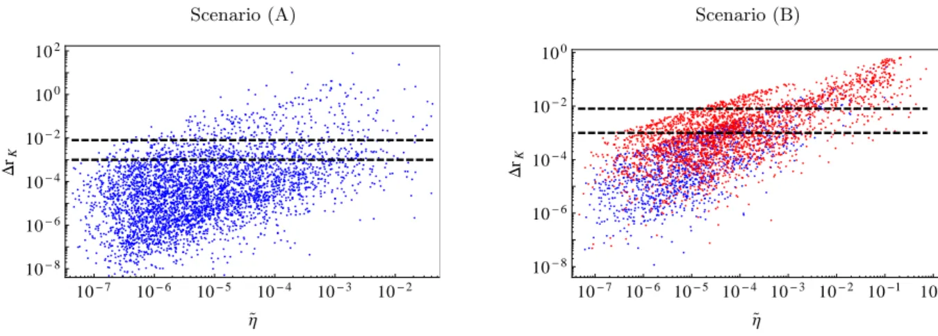
In Figs. 1, we collect our results for ∆rK in scenarios (A) - left panel - and (B) - right
panel, as a function of ˜η, which parametrizes the departure from unitarity of the active neutrino mixing sub-matrix ˜UPMNS, ˜η = 1 − |Det( ˜UPMNS)|. Although the cosmological constraints are
not always satisfied, we stress that all points displayed comply with the different experimental and laboratory bounds discussed before. For the case of scenario (A), one can have very large
Scenario (A) Scenario (B) 10- 7 10- 6 10- 5 10- 4 10- 3 10- 2 10- 8 10- 6 10- 4 10- 2 100 102 Η D rK 10- 7 10- 6 10- 5 10- 4 10- 3 10- 2 10-1 100 10- 8 10- 6 10- 4 10- 2 100 Η D rK
Figure 1. Contributions to ∆rK in the inverse seesaw as a function of ˜η = 1 − |Det( ˜UPMNS)|:
regimes A (left) and B (right). The upper (lower) dashed line denotes the current experimental limit (expected sensitivity). On the right panel, red points denote cases where Yν &10−2. All
points comply with experimental and laboratory constraints. Points in (B) are also in agreement with cosmological bounds, while those in (A) require considering a non-standard cosmology.
contributions to RK, which can even reach values ∆rK ∼ O(1) (in some extreme cases we
find ∆rK as large as ∼ 100). The hierarchy of the sterile neutrino spectrum in case (A) is
such that one can indeed have a significant amount of LFU violation, while still avoiding non-unitarity bounds. Although this scenario would in principle allow to produce sterile neutrinos in light meson decays, the smallness of the associated Yν (. O(10−4)), together with the loop
function suppression (Gγ), precludes the observation of LFV processes, even those with very
good associated experimental sensitivity, as is the case of µ → eγ. The strong constraints from CMB and X-rays would exclude scenario (A); in order to render it viable, one would require a non-standard cosmology.
Despite the fact that in case (B) the hierarchy of the sterile states is such that non-unitarity bounds become very stringent (since the sterile neutrinos are not kinematically viable meson decay final states), sizeable LFU violation is also possible, with deviations from the SM predictions again as large as ∆rK ∼ O(1). Although one cannot produce sterile states in meson
decays in this case, the large Yν open the possibility of having larger contributions to LFV
observables so that, for example, BR(µ → eγ) can be within MEG reach.
Although we do not explicitly display it here, the prospects for ∆rπ are similar: in the same
framework, one could have ∆rπ ∼ O(∆rK), and thus ∆rπ∼ O(1) in both scenarios. Depending
on the singlet spectrum, these observables can also be strongly correlated: if all the sterile states are either lighter than the pion (as it is the case of scenario (A)) or then heavier than the kaon, one finds ∆rπ ≈ ∆rK. This is a distinctive feature of our mechanism.
5. Concluding remarks
The existence of sterile neutrinos can potentially lead to a significant violation of lepton flavour universality at tree-level in light meson decays. As shown in this study, provided that the active-sterile mixings are sufficiently large, the modified W ℓν interaction can lead to large contributions to lepton flavour universality observables, with measurable deviations from the standard model expectations, well within experimental sensitivity. This mechanism might take place in many different frameworks, the exact contributions for a given observable being model-dependent.
As an illustrative (numerical) example, we have evaluated the contributions to RK in the
hierarchies of the sterile states. Our analysis reveals that very large deviations from the SM predictions can be found (∆rK ∼ O(1)) - or even larger, well within reach of the NA62
experiment at CERN. This is in clear contrast with other models of new physics (for example unconstrained SUSY models, where one typically has ∆rK .O(10−3)).
Acknowledgments
The author is grateful to A. Abada, D. Das, A. M. Teixeira and C. Weiland for their collaboration in the work this talk is based on. This work has been supported by the ANR project CPV-LFV-LHC NT09-508531.
References
[1] V. Cirigliano and I. Rosell, Phys. Rev. Lett. 99 (2007) 231801 [arXiv:0707.3439 [hep-ph]]. [2] M. Finkemeier, Phys. Lett. B 387 (1996) 391 [hep-ph/9505434].
[3] E. Goudzovski [NA48/2 and NA62 Collaboration], PoS EPS HEP2011 (2011) 181 [arXiv:1111.2818 [hep-ex]]. [4] G. Czapek et al., Phys. Rev. Lett. 70 (1993) 17.
[5] E. Goudzovski [NA48/2 and NA62 Collaborations], arXiv:1208.2885 [hep-ex]. [6] D. Pocanic et al., arXiv:1210.5025 [hep-ex].
[7] C. Malbrunot et al., AIP Conf. Proc. 1441 (2012) 564. [8] W. -S. Hou, Phys. Rev. D 48 (1993) 2342.
[9] A. Masiero, P. Paradisi and R. Petronzio, Phys. Rev. D 74 (2006) 011701 [hep-ph/0511289]. [10] A. Masiero, P. Paradisi and R. Petronzio, JHEP 0811 (2008) 042 [arXiv:0807.4721 [hep-ph]]. [11] J. Ellis, S. Lola and M. Raidal, Nucl. Phys. B 812 (2009) 128 [arXiv:0809.5211 [hep-ph]]. [12] J. Girrbach and U. Nierste, arXiv:1202.4906 [hep-ph].
[13] R. M. Fonseca, J. C. Romao and A. M. Teixeira, Eur. Phys. J. C 72 (2012) 2228 [arXiv:1205.1411 [hep-ph]]. [14] J. Schechter and J. W. F. Valle, Phys. Rev. D 22 (1980) 2227; M. Gronau, C. N. Leung and J. L. Rosner,
Phys. Rev. D 29 (1984) 2539.
[15] R. E. Shrock, Phys. Lett. B 96 (1980) 159; R. E. Shrock, Phys. Rev. D 24 (1981) 1232.
[16] A. Abada, D. Das, A. M. Teixeira, A. Vicente and C. Weiland, JHEP 1302 (2013) 048 [arXiv:1211.3052 [hep-ph]].
[17] T. Asaka, S. Blanchet and M. Shaposhnikov, Phys. Lett. B 631 (2005) 151 [hep-ph/0503065]. [18] A. Ibarra, E. Molinaro and S. T. Petcov, JHEP 1009 (2010) 108 [arXiv:1007.2378 [hep-ph]]. [19] R. N. Mohapatra and J. W. F. Valle, Phys. Rev. D 34 (1986) 1642.
[20] D. V. Forero, M. Tortola and J. W. F. Valle, Phys. Rev. D 86 (2012) 073012 [arXiv:1205.4018 [hep-ph]]. [21] A. Atre et al., JHEP 0905 (2009) 030 [arXiv:0901.3589 [hep-ph]].
[22] A. Kusenko, Phys. Rept. 481 (2009) 1 [arXiv:0906.2968 [hep-ph]].
[23] S. Antusch, J. P. Baumann and E. Fernandez-Martinez, Nucl. Phys. B 810 (2009) 369 [arXiv:0807.1003 [hep-ph]].
[24] J. Adam et al. [MEG Collaboration], Phys. Rev. Lett. 107 (2011) 171801 [arXiv:1107.5547 [hep-ex]]. [25] A. Ilakovac and A. Pilaftsis, Phys. Rev. D 80 (2009) 091902 [arXiv:0904.2381 [hep-ph]].
[26] D. N. Dinh, A. Ibarra, E. Molinaro and S. T. Petcov, JHEP 1208 (2012) 125 [arXiv:1205.4671 [hep-ph]]. [27] R. Alonso, M. Dhen, M. B. Gavela and T. Hambye, JHEP 1301 (2013) 118 [arXiv:1209.2679 [hep-ph]]. [28] A. Ilakovac, A. Pilaftsis and L. Popov, arXiv:1212.5939 [hep-ph].
[29] M. Hirsch, F. Staub and A. Vicente, Phys. Rev. D 85 (2012) 113013 [arXiv:1202.1825 [hep-ph]]. [30] A. Abada et al., JHEP 1209 (2012) 015 [arXiv:1206.6497 [hep-ph]].
[31] A. Ilakovac and A. Pilaftsis, Nucl. Phys. B 437 (1995) 491 [hep-ph/9403398]. [32] F. Deppisch and J. W. F. Valle, Phys. Rev. D 72 (2005) 036001 [hep-ph/0406040]. [33] J. Beringer et al. [Particle Data Group Collaboration], Phys. Rev. D 86 (2012) 010001.
[34] P. S. Bhupal Dev, R. Franceschini and R. N. Mohapatra, Phys. Rev. D 86 (2012) 093010 [arXiv:1207.2756 [hep-ph]].
[35] F. del Aguila, J. de Blas and M. Perez-Victoria, Phys. Rev. D 78 (2008) 013010 [arXiv:0803.4008 [hep-ph]]. [36] A. Y. Smirnov and R. Zukanovich Funchal, Phys. Rev. D 74 (2006) 013001 [hep-ph/0603009].
[37] G. Gelmini et al., JCAP 0810 (2008) 029 [arXiv:0803.2735 [astro-ph]]. [38] D. V. Forero et al., JHEP 1109 (2011) 142 [arXiv:1107.6009 [hep-ph]]. [39] J. A. Casas and A. Ibarra, Nucl. Phys. B 618 (2001) 171 [hep-ph/0103065].