Proceedings of the ASME 2011 International Design Engineering Technical Conferences & Computers and Information in Engineering Conference IDETC/CIE 2011 August 29-31, 2011, Washington, DC, USA
DETC2011-48313
SIMULATION OF DIFFERENTIALS IN FOUR-WHEEL DRIVE VEHICLES USING
MULTIBODY DYNAMICS
Geoffrey Virlez∗
Olivier Br ¨uls Pierre Duysinx
Department of Aerospace and Mechanical Engineering (LTAS) University of Li `ege
Chemin des chevreuils, 1, B52/3, 4000 Li `ege Belgium
Email: [email protected]
Nicolas Poulet
JTEKT Torsen Europe S.A. Rue du grand peuplier, 11
Parc industriel de Str ´epy 7110 Str ´epy-Bracquegnies
Belgium
Email: [email protected]
ABSTRACT
The dynamic performance of vehicle drivetrains is signifi-cantly influenced by differentials which are subjected to complex phenomena. In this paper, detailed models of TORSEN differ-entials are presented using a flexible multibody simulation ap-proach, based on the nonlinear finite element method. A cen-tral and a front TORSEN differential have been studied and the numerical results have been compared with experimental data obtained on test bench. The models are composed of several rigid and flexible bodies mainly constrainted by flexible gear pair joints and contact conditions. The three differentials of a four wheel drive vehicle have been assembled in a full drivetrain in a simplified vehicle model with modeling of driveshafts and tires. These simulations enable to observe the four working modes of the differentials with a good accuracy.
INTRODUCTION
Nowadays the requirements to reduce fuel consumption and environmental pollution are more and more important in auto-motive industry. In order to reach this goal, the current trend addresses the enhancement of reliable simulation tools in the de-sign process. Multibody simulation techniques are often used for
∗Address all correspondence to this author.
dynamic analysis of suspensions and engines. The link between engine and wheels of the vehicle is the drivetrain. The model-ing of transmission components, such as differential, gear box or clutch would allow the global modeling of cars from the motor to the vehicle dynamics.
Differentials are critical components whose behavior influ-ences the dynamics of vehicles. They are subjected to many non-linear and discontinuous phenomena: impact, hysteresis, contact with friction, backlash,... Some vibrations can notably be gen-erated and transmitted in the whole car structure and decrease the comfort of the passengers. An accurate mathematical model is needed to improve the performance of these mechanical sys-tems and decrease their weight. Nevertheless the modeling of discontinuities and nonlinear effects is not trivial and often leads to numerical problems.
The literature mentions several ways to model transmission components in automotive and other application fields such as wind turbines or railway. The gear contacts can be modeled with fully elastic model of gear wheels as described in [1]. Gear pairs are sometimes represented with a purely rigid behavior (see [2]) or with modal models to study the vibrations [3]. Modeling of multi-stage planetary gears trains are available in [4] and [5]. Reference [6] presents a method to simulate impacts in gear trains following several approaches. Methods to deal with
nu-merical problems due to non-smooth phenomena such as impacts between bodies are explained in [7], [8]. Impacts modeling be-tween bodies is carried out in [9].
The objective of this paper is to develop accurate models of TORSEN differentials able to simulate the locking effects of these limited slip differentials. In order to take the flexibility of the system into account, the nonlinear finite element method based on absolute nodal coordinates has been used [10]. This method is implemented in SAMCEF/MECANO and allows the modeling of complex mechanical systems composed of rigid and flexible bodies, kinematics joints and force elements. The nu-merical solution is based on a Newmark-type integration scheme with numerical dissipation, which is combined with a regulariza-tion of discontinuities and non-smooth phenomena in the system. The sequel of this paper is organized as follows. The next section will describe the working principle of TORSEN differ-entials with a particular attention to type C and type B which have been modeled in this work. Then the formulation used to model gear pairs and contact conditions, the two main joints in-cluded in the system, will be looked over. The various models are described in detail before the analysis and validation of the simulation results. Finally, the three differentials of a four-wheel drive vehicle have been assembled in a full drivetrain model and a simulation of vehicle displacement is carried out.
DESCRIPTION OF THE APPLICATION: TORSEN DIF-FERENTIALS
The two essential functions of any differential are: transmit the motor torque to the two output shafts and allow a difference of rotation speed between these two outputs. In a vehicle, this mechanical device is particularly useful in turn when the outer wheels have to rotate quicker than the inner wheels to ensure a good handling.
The main drawback of a conventional differential (open dif-ferential) is that the total amount of available torque is always split between the two output shafts with the same constant ra-tio. In particular, this is a source of problems when the driving wheels have various conditions of adherence. If the motor torque exceeds the maximum transferable torque limited by road fric-tion on one driving wheel, this wheel starts spinning. Although they don’t reach their limit of friction, the others driving wheels are not able to transfer more torque because the input torque is often equally splitted between the two output shafts.
The TORSEN differentials enable to reduce significantly this undesirable side effect. This kind of limited slip differen-tial allows a variable distribution of motor torque depending on the available friction of each driving wheel. For a vehicle with asymmetric road friction between the left and right wheels, for example, right wheels are on a slippery surface (snow, mud...) whereas left wheels have good grip conditions, it is possible to transfer an extra torque to the left lane. That allows the
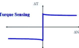
vehi-FIGURE 1. LOCKING EFFECT OF TORSEN DIFFERENTIAL (WHEN T1+T2 IS CONSTANT)
cle to move forward whereas it would be hardly possible with a open differential. However, the overall driving torque can’t be applied on one output shaft while no load is submitted to the second shaft. When the difference between the 2 output torques becomes too large, the differential unlocks and lets different ro-tation speeds but keeps the same constant torque ratio (see Fig-ure 1). The maximum ratio of torque imbalance permitted is defined by a constant, the Torque Distribution Ratio (TDR), spe-cific for each differential design.
T DR=T2 T1
(1)
where T2and T1are respectively the highest and lowest output torques.
A T DR = 4 means that one side of the differential can han-dle up to 80% while the other side would have to hanhan-dle only 20% of the applied torque. During acceleration under asymmet-ric traction conditions, no relative wheelspin will occurs as long as the higher traction side can handle the higher percentage of ap-plied torque. When the traction difference exceeds the TDR, the slower output side of the differential receives the tractive torque of the faster wheel multiplied by the TDR; any extra torque re-maining from applied torque contributes to the angular accelera-tion of the faster output side of the differential. In turn, due to the centrifugal force, a transfer of loads modifies the distribution of normal loads on the wheels, which also induces different friction potentials.
When a TORSEN differential is used, the torque biasing is always a precondition before any difference of rotation speed between the two output shafts. Contrary to viscous coupling, TORSEN (a contraction of Torque-Sensing) is an instantaneous and pro-active process which acts before wheel slip.
The differentials can be used either to divide the drive torque into equal parts acting on the traction wheels of the same axle, or to divide the output torque from the gearbox between the two axles of four-wheels drive vehicles. This second application is often called the transfer box differential or central differential.
In this work, the type C TORSEN differential has been stud-ied for the central differential and the type B for the front and
rear axle differentials. These components are manufactured by the company JTEKT TORSEN S.A. and notably equip the Audi Quattro.
As depicted on Figure 2, the type C TORSEN is composed of a compact epicyclic gear train which allows a non-symmetric distribution of the torque due to the various number of teeth on the ring gear and the sun gear. The differential under study tends to provide more torque (58%) to the rear axle than to the front axle and therefore favour a rear wheel drive behavior.
Due to the axial force produced by the helical mesh, several gear wheels can move axially and enter in contact with the var-ious thrust washers fixed on the case or housing. The friction encountered by this relative sliding is at the origin of the locking effect of TORSEN differentials. The second important contribu-tion to the limited slip behavior is due to the friccontribu-tion between the planet gears and the housing holes in which their are inserted. When one axle tries to speed up, all encountered frictions tend to slow down the relative rotation and involve a variable torque distribution between the output shafts. The biasing on the torque only results from the differential gearing mechanical friction.
This limited slip differential has four working modes which depend on the direction of torque biasing and on the drive or coast situation. According to the considered mode, the gear wheels rub against one or the other thrust washers which can have different friction coefficients and contact surfaces. The fric-tion torque changes for each working mode which influences the TDR as it will be shown in the sequel of this paper.
For front and rear differentials, the type B TORSEN is used to transfer the driving torque to the left and right wheels of a same axle. It also includes gear pairs with helical meshing and thrust washers but is not based on an epicyclic gear train (see Figure 3). This mechanism must be symmetric between the right and the left half axle in a static case because there isn’t any rea-son to favor one lane rather than the other. The element gears are assembled by pairs and they mesh each other at their two extrem-ities. The central part is composed of a slick reduced section and a toothed portion which meshes with one of the two side gears linked respectively to the right or left wheel. The working princi-ple is similar to type C central differential. The locking is created by the friction between the elements gears and housing cavities as well as between the annular lateral contacts face of the sides gears and the thrust washers. This TORSEN differential has also four working modes. It is possible to provide more torque to the right or to the left wheel and for each case the drive and coast situation must be considered.
FINITE ELEMENT METHOD IN MULTIBODY SYSTEMS For differentials, as for most automotive transmission com-ponents, it can be interesting to take flexibility in the system into account. For instance, the backlash between teeth in gear pairs and impact phenomena can generate some vibrations and noise
FIGURE 2. KINEMATIC DIAGRAM, EXPLODED DIAGRAM AND CUT-AWAY VIEW OF TYPE C TORSEN DIFFERENTIAL
which could be transmitted to the whole power train. In order to represent these physical phenomena, some bodies like the trans-mission shafts should be considered as flexible. The numerical model should also be able to manage the nonlinearities and high discontinuities, e.g. the stick-slip phenomenon.
In this work, the approach chosen to model the differen-tials is based on the nonlinear finite element method for flexi-ble multibody systems developed by G´eradin and Cardona [10]. This method allows the modeling of complex mechanical sys-tems composed of rigid and flexible bodies, kinematics joints and force elements. Absolute nodal coordinates are used with respect to a unique inertial frame for each model node. Hence, there is no distinction between rigid and elastic coordinates which allows accounting in a natural way for many nonlinear flexible effects and large deformations. The cartesian rotation vector combined with an updated lagrangian approach is used for the parametriza-tion of rotaparametriza-tions. This choice enables the representaparametriza-tion of large rotations.
This approach to model flexible multibody systems is im-plemented in the software SAMCEF/MECANO commercialised by SAMTECH S.A. The discontinuities are managed with reg-ularizations and the equations of motion for a dynamic system
FIGURE 3. EXPLODED DIAGRAM OF TYPE B TORSEN DIF-FERENTIAL
subjected to holonomic constraints are stated in the form: M(q) ¨q+ ggyr(q, ˙q) + gint(q, ˙q) + φqT(pφ + kλ ) = gext(t) (2)
k φ (q,t) = 0 (3) where q, ˙qand ¨qare the generalized displacement, velocities and acceleration coordinates, M(q) is the mass matrix, ggyris the gy-roscopic and complementary inertia forces, gint(q, ˙q) the internal forces, e.g. elastic and dissipations forces and gext(t) the ex-ternal forces. According to the augmented lagrangian method, the constraint forces are formulated by φT
q(pφ + kλ ) where λ is the vector of Lagrange multiplier related to algebraic constraints φ = 0; k and p are respectively a scaling and a penalty factor to improve the numerical conditioning.
Equations (2) and (3) form a system of nonlinear differential-algebraic equations. The solution is evaluated step by step using a second order time integration scheme. For this study, the Chung-Hulbert scheme, a generalized α-method has been used (see References [11], [12]). At each time step, a sys-tem of nonlinear algebraic equations has to be solved. In order to solve this system, a Newton-Raphson method is used.
In the sequel on this section, the mathematical formulation will be looked over for the two main kinematic joints used in the model of TORSEN differentials: the gear pair element and the contact condition.
Gear pair element
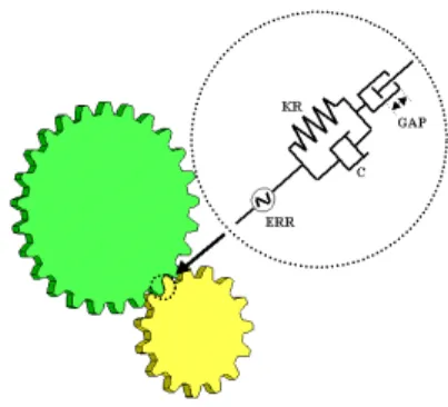
Each gear pair in the differential is modeled as a joint de-fined between two physical nodes: one at the center of each gear wheel considered as a rigid body. Nevertheless the flexi-bility of the gear mesh is accounted for by a nonlinear spring and
FIGURE 4. GEAR PAIR - FLEXIBLE CONTACT LAW ALONG THE LIGNE OF PRESSURE
damper element inserted along the instantaneous normal pres-sure line (see Fig. 4). Several specific phenomena in gear pairs which influence significantly the dynamic response of gears are also included in the model: backlash, mesh stiffness fluctuation, misalignment, friction between teeth.
The formulation developed in [13] and summarized below, is available for describing flexible gear pairs in 3 dimensional analysis of flexible mechanism. Any kind of gears often used in industry can be represented with this formulation: spur gears, helical gears, bevel gears, ring gears, rack-and-pinion... All re-action forces due to the gear engagement are taken into account: tangential, axial and radial forces.
The modeling of gear wheels as flexible bodies and the in-troduction of contact conditions between the flank of teeth would perhaps be possible with a finite element mesh. However, that would increase dramatically the size and the complexity of the model due to the complex and numerous gear meshes. The sim-plified approach with a flexible joint between rigid wheels is suf-ficient to observe the locking effects of the TORSEN differen-tials. The main objective of this study is to develop a global and light differential model able to analyze the dynamical behavior. The differential model will be inserted in a complete driveline modeling of a vehicle model including also frame, suspensions and tire. Local effects such as stress in the gear teeth are not required for this kind of global study.
One triad of unit orthogonal vectors is defined at each wheel center in the reference configuration: (µ1,µ2,µ3) for the first wheel A and (ξ1,ξ2,ξ3) for the second wheel B. The first vectors µ1and ξ1are perpendicularly oriented to the wheel plane. The second vectors µ2and ξ2point towards the contact point and the third vectors µ3and ξ3complete a dextrorsum reference frame (see Fig. 5).
At the current configuration, the orientation of these two tri-ads is obtained multiplying the rotation operator of each wheel by the vectors at the reference configuration:
FIGURE 5. GEAR PAIR KINEMATICS AND SIGN CONVENTIONS FOR CONE AND HELIX ANGLE [14]
with RA, RBare the rotation matrices at nodes A and B. They are related to the rotation vectors ΘA, ΘB through the exponential operator exp( ˜ΘA), exp( ˜ΘB).
Two other unit dextrorsum triads, (µ100, µ200, µ300) and (ξ100, ξ200, ξ300), are defined at the current configuration with the same orientation rules as the reference triads (µ1, µ2, µ3) and (ξ1, ξ2, ξ3). A last unit triad (η100, η
00 2, η
00
3) is also defined at the contact point C. η100 is parallel to the tooth baseline; η200points along the tooth vertical line, from the first wheel to the second one; and η300is normal to the tooth midplane. As shown in Fig. 5, the triad (η100, η200, η300) can be related to the triad (µ100, µ200, µ300) through the helix angle βA and cone angle γA whereas similar relations hold for the triad (ξ100, ξ200, ξ300) through the angles βBand γB. It is then possible to get the triad (ξ100, ξ200, ξ300) of the second wheel from the triad (µ100, µ200, µ300) of the first wheel multiplied by a matrix Z composed of sine and cosine of helix and cone angles of both wheels:
[ξ100 ξ200 ξ300] = [µ100 µ200µ300] Z(γA, γB, βA, βB) (5) The position of the contact point being the same when ex-pressed either in terms of kinematics variables at wheel A or at wheel B (xA
C,xBC), Reference [13] shows that the expressions of the vector µ2, µ3and ξ2, ξ3at the reference configuration can be found in terms of the distance vector xABbetween center wheels, the normal vector to the first wheel plane µ1and geometric pa-rameters of both wheels: βA, βB, γA, γB and rA, rBthe wheel ra-dius.
In order to describe this flexible gear pair joint, fifteen kine-matic variables are used and are grouped together into the gener-alized coordinates vector q,
q= {xTA ΘTA xTB ΘTB ψA ψB um} (6)
where xA, xBand ΘA, ΘBare respectively the position and rota-tion vector of wheel center A and B in the inertial frame. The three remaining generalized coordinates are internal variables. um is a scalar value which represents the deformation of gear mesh in the hoop direction. This variable is in fact a combined measure resulting from tooth deformation at both wheels and clearance between teeth. The angular displacements ψA, ψB mea-sure the relative rotation of wheels A and B in the local frame at-tached to each wheel center. These variables allow to express the following simple relations between quoted and doubly-quoted frames:
µ200= µ20 cos ψA− µ30 sin ψA µ300= µ20 sin ψA+ µ30 cos ψA(7) ξ200= ξ20 cos ψB− ξ30 sin ψB ξ300= ξ20 sin ψB+ ξ30 cos ψB(8)
This joint has twelve physical degrees of freedom: the six components of rigid body motion at each wheel center (xA, xB, ΘA, ΘB) plus the elastic deformation of the mesh minus the rota-tion constraint between wheels. The dimension of the kinematic variable vector q exceeds by three the number of physical de-grees of freedom. Therefore, three kinematic constraints have to be imposed. Three Lagrange multipliers, associated to these constraints, are added to the generalized coordinates q to form the vector of the eighteen unknowns of the joint.
The first algebraic equation of constraint is the kinematic re-lation resulting from teeth contact and gives the rere-lation between angular displacements of booth wheels:
φ1= (−ψAzA+ ψBzB)
mn cos αn
2 + um cos αn= 0 (9) where mnis the normal module of the gear teeth, αnthe pressure angle in the normal plane, and zAand zBare the numbers of teeth
at each wheel. It can be shown easily that by formulating the constraint in this way, the associated Lagrange multiplier (scaled by factor k) has the physical meaning of a normal contact force: F = kλ1.
The second constraint represents the hoop contact constraint produced by engagement between teeth:
φ2= (xAC− xBC).η 00A
3 = 0 (10)
where xCA, xB
C give the position of the contact point computed on wheel A and B, respectively.
The third constraint expresses that the triad (η100, η200, η300) is unique, when computed in terms of kinematic variables of either wheel:
φ3= η200A.η 00B
3 = 0 (11)
The mesh force is derived from the elastic potential νm, de-fined as follows:
νm= 1
2km[[um+ xerr]]
2 (12)
with the operator [[•]] defined as
[[x]] = x x≥ 0 0 b< x < 0 x+ b x≤ −b (13)
where kmis the mesh stiffness and b is the hoop backlash. xerr is the loaded transmission error which includes both the mesh errors with respect to the theoretical gear profiles and time varia-tion effects of mesh stiffness due to the variavaria-tion of the number of teeth in contact. This effect is included in the form of a displace-ment excitation representing the fundadisplace-mental harmonic which is assumed to be a function of the angular displacement at one gear (φAfor example).
xerr(ψA) = X (1 − cos(zAψA)) (14)
Mesh damping force is accounted for by adding a term cmu˙mto the internal forces (cmbeing the damping coefficient).
The hoop and axial components of the contact force oriented along ν300, have been taken into account when formulating the holonomic constraint φ2. However, the radial component of the contact force is of non-holonomic nature and has to be added explicitly to the formulation as a non-conservative force. The radial component of the force acting on wheel A at the contact
FIGURE 6. CONTACT CONDITION - PROJECTION OF SLAVE NODE ON MASTER SURFACE
point is F = −k|λ1| sin α2η200while the opposite force −F acts upon wheel B at the same point.
If the mutual sliding speed along teeth in contact is non-zero (e.g. worm gears), a non-negligeable friction force between wheels appears:
Ff r= −sign(vrel) µ(vrel) k|λ1| η100 (15)
vrelis the relative sliding speed, measured along the teeth lon-gitudinal direction η100
µ (vrel) is the friction coefficient for which a regularization is used to avoid discontinuities while the sign of vrel is chang-ing.
This friction force takes place in the internal forces of the gear pair element and is of non-holonomic nature.
Contact element
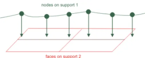
In the software used, contacts can be defined between a rigid structure and a flexible part (flexible/rigid contact) or between two flexible parts (flexible/flexible contact). Contact relations are created between a set of nodes on the first support that will be connected to a facet (in case of flexible/flexible contact) or a surface (in case of flexible/rigid contact) on the second support. Contact algorithms consist of two steps: the first one searches for the projection of each slave node in the master surface(s) and creates an associated distance sensor, the second step imposes the kinematic constraint. In the nonlinear case (large displace-ments, large rotations), the contact is treated as a nonlinearity and the coupled iterations method is used. A contact element is created, with a kinematic constraint that is active when contact and inactive without contact.
In order to model the Torsen differential, the friction has to be taken into account in all contact conditions. In this case, in addition to a distance sensor some sliding sensors are generated. The friction force Ff ris directly proportional to the normal reac-tion between the point and the surface by means of a regularized friction coefficient µR(Ff r= µR|Fnorm|). The regularization tol-erance is used to avoid the singularity of the derivative when the relative sliding velocity is zero.
In case of convergence problem, the use of a penalty func-tion allows small interferences. Physically, a penalty funcfunc-tion behaves as a spring that is active in compression but not in trac-tion. Damping is sometimes used to have a smoother response and consequently better convergence properties.
MULTIBODY MODELING OF DIFFERENTIALS
In this work, a complete modeling of the type B and C TORSEN differentials has been carried out with the software SAMCEF Field and its module MECANO for implicit nonlin-ear analysis. These two multibody models are mainly composed of rigid bodies, only the various trust washers are considered with a flexible behavior. The objective of the initial study was to develop a robust modeling approach able to simulate the four working modes and the locking effect of TORSEN differentials. Therefore, several hypotheses which appear reasonable for the analysis of the global working of differentials have been intro-duced.
The axial displacement of planet gears in type C (Fig. 2) and element gears in type B (Fig. 3) have small magnitude and have been locked in the model. The friction coefficient of all contact conditions introduced in the models have been chosen in accordance to experimental data provided by the manufacturer JTEKT TORSEN. Some washers have completely different fric-tion coefficients on their two opposite faces (for example: 0, 1 on one side and 0, 03 on the other side). In this case, only the contact condition with the lower friction coefficient is modeled while the washer is considered to be fixed on the body in con-tact with the other washer face having higher friction coefficient (in Fig. 2 washer #8 is fixed on the sun gear and washer #10 is fixed on the coupling). The planet gears and element gears are inserted in holes of the housing. The joints have been model as hinges even though there is not physical rotation axis in the real system.
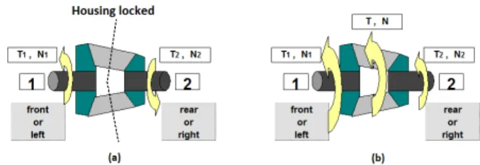
In order to validate and to check the accuracy of the math-ematical model, the numerical results have been compared with measurements on an experimental test bench. For this purpose, the test bench configuration has been recreated in simulations. Contrary to operation in a vehicle, the housing does not rotate during the test (Fig. 7). However, it is nevertheless possible to observe the four working modes because the locking effect of TORSEN differentials is due to relative motions and forces be-tween the output shafts and the housing.
Dynamic analysis has been perform using the Chung-Hulbert generalized-α integration scheme. Due to the presence of gear elements and contact conditions with friction, the tangent matrix is not symmetric and therefore a non-symmetric resolu-tion algorithm has been chosen. This opresolu-tion is computaresolu-tionally more expensive since it increases the number of arithmetic op-erations. But it permits a better convergence in some complex situations such as high Coulomb friction.
FIGURE 7. (A) CONFIGURATION ON TEST BENCH (B) CON-FIGURATION ON VEHICLE
Central Differential : Type C TORSEN
The model of the type C Torsen differential includes in total 15 bodies: 11 rigid bodies and 4 flexible ones (thrust washers). It also includes: 8 gear pairs, 5 contact conditions (flexible/rigid), 4 hinge joints, 1 screw joint. The number of configuration pa-rameters amounts to 8161. The flexible bodies are meshed with volume finite elements obtained by extrusion.
For each gear pair element, the mesh stiffness and damp-ing have been computed accorddamp-ing to the ISO 6336 standard (method B). These parameters depend on material properties and geometrical characteristics (addendum, number of teeth, helical and pressure angles...) of gear wheels and teeth.
In configuration on test bench, a torque is applied to one output shaft whereas the rotation speed of the second shaft is prescribed, which is equivalent to apply a resistant torque. This torque is measured and used to compute the TDR defined in Eq. 1. This index represents the torque distribution due to the locking effects and is simply computed with the applied torque value divided by the resistant torque measured value.
For instance, Figure 8 depicts the case where a torque of 125 Nm is applied to the coupling and the rotation speed of the sun gear is controlled in order to keep a difference of 20 r.p.m. be-tween the two output shafts. The housing and the case are locked in translation and rotation. The sun gear being linked to the front axle and the coupling to rear axle, this situation corresponds to a torque biasing to the rear axle. According to the direction of the torque applied, it is a drive or a coast mode. With the inertial frame used in this simulation, a positive torque involves a drive mode and a negative one, a coast mode.
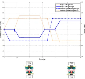
The TDR is a constant specific for each locking mode what-ever the amplitude of the torque applied and the output shafts relative rotation (cf. Fig. 1). The choice of 125 Nm and 20 r.p.m. is only due to the capacity of the experimental test bench used for this work. The time evolution of the applied torque and pre-scribed rotation speed has been chosen to observe the two modes with biasing to rear axle in a same simulation and in order to have a smooth transition between the 2 modes. The parts of in-terest to compute the TDR are the steady state parts 0, 4s − 1s and 2, 2s − 2, 8s.
FIGURE 8. SIMULATION OF TYPE C ON TEST BENCH FOR DRIVE TO REAR AND COAST TO REAR MODES
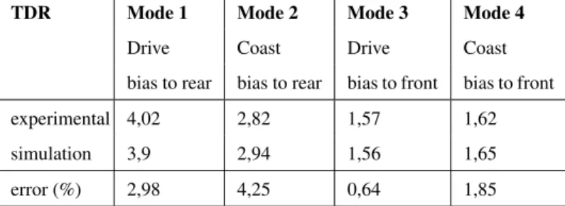
TABLE 1. COMPARISON OF TORQUE DISTRIBUTION RATIOS FOR THE FOUR WORKING MODES (TYPE C TORSEN)
TDR Mode 1 Mode 2 Mode 3 Mode 4
Drive Coast Drive Coast
bias to rear bias to rear bias to front bias to front
experimental 4,02 2,82 1,57 1,62
simulation 3,9 2,94 1,56 1,65
error (%) 2,98 4,25 0,64 1,85
with torque biasing to front axle but are not depicted in this paper. This time, the torque is applied to the sun gear and the rotation speed of the coupling is regulated. For each locking mode, Table 1 shows the good agreement between the simulated TDR values and the experimental results.
This simulation is also able to compute the contact pressure, friction stress, dissipated power, sliding velocity... Figure 9 il-lustrates the contact pressures for all the contact elements intro-duced in the model for the drive to rear mode.
The dynamic response of this differential has also been stud-ied in the vehicle configuration. In this case, the housing is rotat-ing and linked with splines to the propeller shaft which transmits the motor output torque from the gear box. For this kind of simu-lation, a torque is applied to the housing and the rotation speed of the two output shafts is prescribed. In order to observe the four working modes during the same simulation, the time evolution of the three loadings depicted in Fig. 10 has been used.
FIGURE 9. CONTACT PRESSURE ON THRUST WASHERS FOR DRIVE TO REAR MODE (TEST BENCH CONFIGURATION AT TIME T = 0.6 s)
According to the orientation of the inertial frame employed, the rotation speeds have negative values when the vehicle moves forward. The difference of rotation speed has been chosen ar-bitrarily because it doesn’t affect the TDR. The motor torque is positive in coast conditions and negative for drive modes. In or-der to test the robustness of the model, an intermediate level is introduced during the increase and decrease stage of the motor torque. Figure 10 shows the torques on the two outputs (sun gear and coupling), the sum of theses two values at each time step is equal to the value of the torque applied to the housing. The gap between these curves is representative of the torque bi-asing and their ratio gives the TDR. The values computed by this simulation are very close to the values obtained in test bench ex-periments (see. Table 1). In drive modes, more torque is sent to the slower axle while it is the opposite for coast modes. Contrary to the situation on test bench, the two output shafts have same rotation directions as well as the housing whose rotation speed is always determined by the ratio of teeth number on the sun gear and internal gear.
As seen in Figure 11, as soon as the sign of the torque ap-plied to the housing changes, three gear wheels move axially very quickly and involve impacts onto the thrust washers. Some spikes can be seen on the torque curves in several Figures and are due to the transient behavior at the impact time. The discon-tinuity created can affect the convergence of the simulation. The automatic time step decreases significantly and sometimes can’t override the discontinuity. The solution adopted to try to reduce these numerical problems consists in allowing a small penetra-tion of the bodies in contact by a contact stiffness and introduce a damping factor which anticipates slightly the contact in order to reduce the shock. The axial displacements of the sun gear and the coupling are always in the direction and opposite to the in-ternal gear. The sun gear and the coupling are then in contact for
FIGURE 10. TIME EVOLUTION OF TORQUE AND ROTA-TION SPEED OF HOUSING AND OUTPUT SHAFTS OF TYPE C TORSEN ON VEHICULE CONFIGURATION
FIGURE 11. AXIAL DISPLACEMENTS OF GEAR WHEELS (VE-HICLE CONFIGURATION)
all the working modes. This contact has a very low friction coef-ficient (0,03) which allows to reduce the stick-slip phenomenon.
Front or Rear Differential : Type B TORSEN
The type B TORSEN differential has been modeled with 20 bodies (17 rigid, 3 flexible) and the main kinematic constraints are: 10 hinges, 2 cylindrical joints, 3 rigid-flexible contacts
con-TABLE 2. COMPARISON OF TORQUE DISTRIBUTION RATIOS FOR THE FOUR WORKING MODES (TYPE B TORSEN)
TDR Mode 1 Mode 2 Mode 3 Mode 4
Drive Coast Drive Coast
bias to right bias to right bias to left bias to left
experimental 1,6 1,7 1,6 1,7
simulation 1,58 1,66 1,61 1,64
error (%) 3,20 2,35 0,62 3,53
ditions and 20 gear pairs. The model is composed of 21164 con-figuration parameters. This large number of parameters is due to the finite element method for flexible multibody systems used in this work. Indeed, three translational degrees of freedom are re-lated to each node of the flexible bodies. The contact conditions also increase the number of parameters because several internal variables (Lagrange multipliers, distance captor, ...) are intro-duced for each slave node projected on the master surface.
A ring gear fixed on the housing allows the input torque to be transfered to the differential with a hypoid gear mesh. The pinion is fixed on the propeller shaft coming out of the gear box in a front wheel drive vehicle or on a output shaft of central dif-ferential for four wheel drive vehicle. The two side gears are linked with splines to the semi-axles supplying the motor torque to the right and left wheels.
In order to validate the model, the tests on experimental test bench have been reproduced using the simulation tool. The pro-cedure is similar to the one explained in the previous section for the type C TORSEN. The housing is fixed and o torque is applied Figure 12 depicts the resistant torque on the output shaft (side gear left) whose rotation speed is prescribed. The TDR for the four working modes have been computed on the basis of these simulations on test bench. The TDR values computed are close to experimental data as shown on Table 2. The geometrical configuration of the type B TORSEN being symmetric in relation to the output shafts, the TDR values for the modes with torque biasing to the left are similar to the modes with torque biasing to the right. The friction coefficients have similar values for all contacts with thrust washers, which explains the very small dif-ference between the TDR for drive and coast modes.
The configuration on vehicle has also been simulated for this front differential. A torque is applied on the housing and the side gears rotation speeds are prescribed (see Fig. 13). Although very seldom effective in reality, the four locking modes can be observe in backwards motion of the vehicle. The TDR values for theses modes are of course the sames as for vehicle forwards motion. In the second part of the simulation (34s − 67s), the direction of prescribed rotation speed of side gears has been changed which enables to reproduce the differential behavior in backwards mo-tion. Time evolutions of resistant torque on the two side gears are
FIGURE 12. SIMULATION OF TYPE B TORSEN ON TEST BENCH FOR DRIVE AND COAST MODES WITH TORQUE BIAS-ING TO THE RIGHT WHEEL
FIGURE 13. TIME EVOLUTION OF TORQUE AND ROTA-TION SPEED OF HOUSING AND OUTPUT SHAFTS OF TYPE B TORSEN ON VEHICULE CONFIGURATION
symmetric in relation to the middle of the simulation (t = 34s). This proves that the model is able to represent also the locking effects in backwards motion with accurate TDR.
FIGURE 14. ACADEMIC FOUR-WHEEL DRIVE VEHICLE MODEL WITH THREE DIFFERENTIALS
TORSEN DIFFERENTIALS INCLUDED IN A SIMPLE VE-HICLE DRIVETRAIN
As final application of this paper, a global four-wheel drive vehicle equipped with three TORSEN differentials has been modeled (Figure 14).
The objective of this model is to observe the distribution of the engine torque between the four wheels. In this context, a very simplified vehicle model is considered here. The car body is modeled by a lumped mass and the suspension mechanisms are ignored. The differentials are attached to the vehicle frame with hinge joints. In order to connect the central differential (type C) with the front and rear differentials (type B), the driveshafts are represented by rigid bodies as well as the half-axles linking the differentials. Simple tire models are also considered in this simulation.
As depicted on Fig. 15, a driving torque of 100 Nm is applied to the housing of central differential. Friction coefficients are prescribed with a different value for each wheel-ground contact. For this academic application, very different friction coefficients have been assigned arbitrarily to illustrate the torque biasing be-havior of the limited slip bebe-havior. For the shake of simplicity, the drive ratios have been chosen equal to one for the conical gear pairs which mesh the housing of front and rear differen-tials with pinion fixed on driveshafts of the central differential. Friction coefficients in all contact conditions have been modified compared with the previous models with the consequence that the TDR values are modified with repect to Tables 1 and 2.
The torque provided to each wheel is different and the dis-tribution of the motor torque is in accordance with the ground-wheel friction coefficient. The ground-wheel with the higher road fric-tion gets more torque than the others which is the advantage of TORSEN differentials. With open differentials without slip lim-itations the torque on each wheel would be limited by the lowest friction potential (front left wheel) and any extra motor torque contributes to wheel spin up.
FIGURE 15. TORQUE DISTRIBUTION ON EACH WHEEL FOR A FOUR-WHEEL DRIVE VEHICLE EQUIPPED WITH THREE TORSEN DIFFERENTIALS
CONCLUSION AND PERSPECTIVES
Dynamic simulations of TORSEN differentials have been carried out in this work. Those complex mechanical devices in-clude various gear pairs and thrust washers. The friction phe-nomena play a key role in the locking effect. TORSEN differ-entials have been modeled with a flexible multibody approach using the nonlinear finite element method. The flexible gear pair formulation and rigid-flexible contact element which are key el-ement of the modeling, are well adapted to render the four work-ing modes of these limited slip differentials.
The comparison of simulation results with experimental data obtained on test bench has shown a good correlation and there-fore has allowed validating the models and checking their ac-curacy. Finally, the three differentials (front, central and rear) of a four-wheel drive vehicle have been assembled with sim-ple driveshafts and tire models in order to simulate the global behavior of this part of the drivetrain. These simulations have illustrated the working behavior of TORSEN differentials. Al-though the number of configuration parameters is high (several thousands), the computational load required for the simulations appears to be compatible with industrial requirements. The com-putational time for simulations on test bench is about 15 minutes and reaches two hours for simulations in vehicle configuration.
Future work will address the modeling of other mechanical components such as clutch or gear box to complete the full drive-line model. It is also planned to carry out a combined simulation of the vehicle and driveline dynamics to investigate the interac-tion between the two systems during dynamics maneuvers (e.g. elk test).
ACKNOWLEDGMENT
The author, Geoffrey Virlez would like to acknowledge the Belgian National Fund for Scientific research (FRIA) for its fi-nancial support.
REFERENCES
[1] Ziegler, P., and Eberhard, P. “Using a fully elastic gear model for the simulation of gear contacts in the framework of a multibody simulation program”. In The First Joint International Conference on Multibody System Dynamics, May 25-27, 2010, Lappeenranta, Finland.
[2] Perera, M., De la Cruz, M., Theodossiades, S., Rahnejat, H., and Kelly, P. “Elastodynamic response of automotive transmissions to impact induced vibrations”. In The First Joint International Conference on Multibody System Dy-namics, May 25-27, 2010, Lappeenranta, Finland.
[3] Koronias, G., Theodossiades, S., Rahnejat, H., and Saun-ders, T. “Vibrations of differential units in light trucks”. In The First Joint International Conference on Multibody Sys-tem Dynamics, May 25-27, 2010, Lappeenranta, Finland. [4] Inalpolat, M., and Kahraman, A., 2009. “A theoretical
and experimental investigation of modulation sidebands of planetary gear sets”. Journal of sound and vibration, 323, pp. 667–696.
[5] Peeters, J., Vandepitte, D., and Sas, P., 2005. “Analysis of internal drive train dynamics in a wind turbine”. wind energy, 9(1-2), pp. 141–161.
[6] Ziegler, P., Eberhard, P., and Schweizer, B., 2006. “Simu-lation of impacts in geartrains using different approaches”. Arch Appl Mech, 76, pp. 537–548.
[7] Acary, V., and Brogliato, B., 2008. “Numerical methods for nonsmooth dynamical systems”. Lecture Notes in Applied and Computational Mechanics, 35, p. 540.
[8] Jean, M., 1999. “The non-smooth contact dynamics method”. Comput. Methods Appl. Engrg, 177, pp. 235– 257.
[9] Seifried, R., Schiehlen, W., and Eberhard, P., 2010. “The role of the coefficient of restitution on impact problems in multi-body dynamics”. Proc. IMechE, Part K:J. Multi-body Dynamics, 224, pp. 279–306.
[10] G´eradin, M., and Cardona, A., 2001. Flexible multibody dynamics. John Wiley & Sons.
[11] Chung, J., and Hulbert, G., 1993. “A time integration al-gorithm for structural dynamics with improved numerical dissipation: The generalized-α method”. ASME Journal of Applied Mechanics, 60, pp. 371–375.
[12] Arnold, M., and Br¨uls, O., 2007. “Convergence of the generalized-α scheme for constrained mechanical sys-tems”. Multibody System Dynamics, 18(2), pp. 185–202. [13] Cardona, A., 1995. “Flexible three dimensional gear
mod-elling”. European journal of computational mechanics, 4(5-6), pp. 663–691.
[14] Cardona, A., 1997. “Three-dimensional gears modelling in multibody systems analysis”. International journal for numerical methods in engineering, 40, pp. 357–381.

![FIGURE 5. GEAR PAIR KINEMATICS AND SIGN CONVENTIONS FOR CONE AND HELIX ANGLE [14]](https://thumb-eu.123doks.com/thumbv2/123doknet/6188347.159387/5.918.192.728.105.367/figure-gear-pair-kinematics-sign-conventions-helix-angle.webp)