Science Arts & Métiers (SAM)
is an open access repository that collects the work of Arts et Métiers Institute of Technology researchers and makes it freely available over the web where possible.
This is an author-deposited version published in: https://sam.ensam.eu
Handle ID: .http://hdl.handle.net/10985/16599
To cite this version :
Rafael PENAS, Arnaud GAUDIN, Adrien KREIS, Etienne BALMES - Dissipation in hysteretic rubber mount models - In: European Conference on Constitutive Models for Rubber, France, 2019-06-25 - European Conference on Constitutive Models for Rubber - 2019
Any correspondence concerning this service should be sent to the repository
Dissipation in hysteretic rubber mount models
R. Penas
Groupe PSA, V´elizy-Villacoublay, France
Laboratoire PIMM, Arts et Metiers ParisTech, CNRS, CNAM, HESAM, Paris, France
A. Gaudin
Groupe PSA, V´elizy-Villacoublay, France
A. Kreis
Groupe PSA, Poissy, France
E. Balmes
Laboratoire PIMM, Arts et Metiers ParisTech, CNRS, CNAM, HESAM, Paris, France SDTools, Paris, France
ABSTRACT: Rubber mounts are elements of extreme importance in automotive suspension, and accurate modeling is crucial for comfort design. While mount characterization is typically done using cycles, actual performance is often associated with transients. The paper thus focuses on the impact of power dissipation on suspension models during transients. For scalar or 0D hysteretic models that respect Madelung rules and Masing’s law, a method is introduced to compute instant dissipation even for models where it is not explicitly available. It is shown that stiffness and dissipation depend only on the last turning point and this dependence should be the core aspect for identifying and modeling hysteretic dissipation. The second section introduces two different 0D models having the same full cycle dissipation and force amplitude, thus the same storage and loss moduli in a first harmonic approximation of the mount behavior, though having different instantaneous dissipation. The case of a transient starting torque soliciting a suspended powertrain is finally considered. The different suspension models are shown to have different instant dissipation which might deeply modify the conclusions drawn from the dynamic simulation.
1 INTRODUCTION
Rubber mounts are widely used in automotive indus-try due to their unique combination of moderate stiff-ness and high dissipation. These properties are partic-ularly interesting for softening and filtering vibrations in articulations between moving parts. Despite the in-tense utilization of rubbery materials, their behavior is still subject of active research, given that current mod-eling strategies cannot provide fully predictive design. One of the main modeling demands for this type of articulations comes from multibody simulations where a low computational cost is a modeling con-straint. For this reason, scalar or 0D models are the most commonly used for emulating rubber articula-tions. These models can describe and accumulate dif-ferent nonlinear effects, while keeping a relatively low complexity. Models of this kind are often found in the specific literature such as Coveney & Johnson
(2000), Sj¨oberg (2002), Bourgeteau (2009).
To identify this complex behavior, the most used technique is to impose cyclic solicitations and fit the force response with scalar models. Cyclic identifica-tion does not provide informaidentifica-tion on dissipaidentifica-tion dur-ing transients. The first section describes hysteretic models which are the focus of this work. It is in partic-ular shown how instant dissipation, even if is not ac-cessible experimentally, can be computed and used as a valuable asset for analysis, by giving an estimation of when and where the dissipation is concentrated. The second section describes two models equivalent from the point of view of cyclic dissipation but lead-ing to very different behavior in an engine start simu-lation.
2 HYSTERETIC MODEL
In the scope of this work, hysteresis is taken as a rate-independent behavior that respects the Madelung rules and the Masing’s law (see Brokate & Sprekels (2012)). The rate-independence means that viscoelas-tic contribution is not taken in account and should be object of further work.
The Madelung rules state that :
• Any curve Γ1 emanating from a turning point
A of the force/displacement graph (figure 1) is uniquely determined by the coordinates of A. • If any point B on the curve Γ1 becomes a new
turning point, then the curve Γ2 originating at B
leads back to the point A.
• If the curve Γ1 is continued beyond the point
A, then it coincides with the continuation of the curve Γ which led to the point A before the Γ1− Γ2cycle was traversed.
e
F Γ
Γ1
BΓ2
A
Figure 1: Illustration of Madelung rules
Noting + the curve that leads A to B and − the curve that leads B to A. The cycle closure, or the fact that every turning point must be passed though again before reaching greater deformation, can be written as the integral of the tangent stiffness or slope K(e) = ∂f /∂e over two half cycles
0 = eB R eA K+(e − eA)de + eA R eB K−(e − eB)de = eB−eA R 0 K+(e)de + 0 R eB−eA K−(e)de = eB−eA R 0 (K+(e) − K−(−e)) de (1)
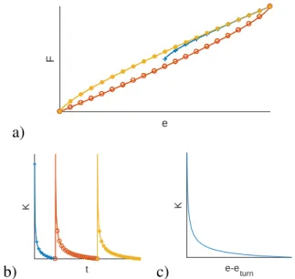
Since this is true for any cycle length, the tangent stiff-ness is an even function of the displacement, that is K+(e) = K−(−e). Thus in figure 2 rather than
dis-playing the classical cycle on the top, one chooses to represent the tangent stiffness.
Other hysteretic model main characteristic is the fact that the first loading curve should be homothetic to the first unloading curve, with a scale factor of two, known as Masing’s law (Brokate & Sprekels 2012). Combining both laws, illustrated in figure 2, one can represent K(e) as a function of distance to turning point with a factor 2 on e when starting from 0.
Concerning dissipation, the parity property is quite useful, since dissipation can be split equally between
a) e F b) t K c) e-e turn K
Figure 2: Illustration of Masing’s law. a) classical cycle, tangent stiffness as function time (b) and distance to turning point (c)
loading and unloading. From any turning point A and current point B, it is possible to close a cycle going back to point A, where dissipation verifies
Ed = eB R eA Fdisde = 12 H F de = 12( eB R eA F+de + eA R eB F−de) = eB R eA F (e)de − F (eB− eA)(eB− eA) (2)
which can be used to compute the instantaneous value of dissipated energy.
These rules are applicable when neglecting vis-coelastic and nonlinear elastic effect. Figure 3 illus-trates tests with triangular enforced displacement. A low, constant speed was used to minimize viscoelas-tic effects which should remain negligible. Nonlinear elastic effects, from both geometric and material na-tures are also negligible due to the use of deforma-tions below 10%. 0 2 4 6 8 10 12 Time [s] -1 -0.5 0 0.5 1 Displacement [mm] -1 -0.5 0 0.5 1 Displacement [mm] -1000 -500 0 500 1000 Force [N]
Figure 3: Imposed displacement and force-displacement re-sponse
The results are shown in the force/displacement plane in figure 3. This plot suggests that the stated hypotheses are plausible, but a simpler verification is to show, as in figure 4, the instant stiffness as function of the distance to the last turning point. In this repre-sentation, the verification of hypotheses is confirmed by the superposition of all curves.
0 0.5 1 1.5 2
Distance to turning point [mm] 1000 1500 2000 2500 3000 Tangent stiffness [N/mm]
Figure 4: Tangent stiffness as function of distance to last turning point
Since the K(e − eturn) curve completely defines an
hysteretic model, a non-parametric representation of the behavior is simply achieved though its discretiza-tion. Segalman (2005) in his work proposes a model based on a rheologic representation, shown in figure 5. This model allows the reproduction of the curve re-specting both laws with a continuous force evolution and control on the accuracy.
e0 k0 k1 Ff1 e1 kn Ffn en
Figure 5: Rheologic scheme for Iwan’s model
Despite needing a high number of Jenkins cells for accurate representation, as seen on figure 6, the low computational effort associated to each cell makes it an interesting model for application purposes.
e-eturn
K
Base curve Iwan 10 cells Iwan 50 cells
Figure 6: Illustration of Iwan’s model response
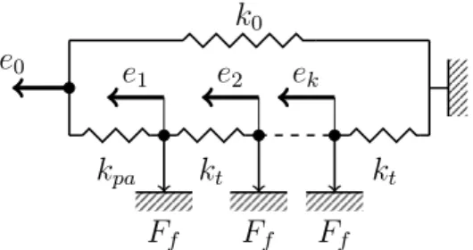
An alternate hysteretic model that respects the stated hypotheses is the STS model, introduced and
detailed by Coveney & Johnson (2000). This model is based on an spring in parallel of an assembly of identical Jenkins cells in series, shown in figure 7. By making the springs stiffness tend to infinity and the friction forces tend to zero, with their product con-stant (ktFf = Ct), one reaches to a continuous model,
defined by the equation 3. k0 e0 e 1 Ff e2 Ff ek kt Ff kt kpa
Figure 7: Rheologic scheme for the STS model
F − Fturn = r N Ct|e − eturn| +2kN Cpat 2 −N Ct 2kpasign(e − eturn) (3)
3 NONLINEAR ELASTICITY AND HYSTERETIC DAMPING
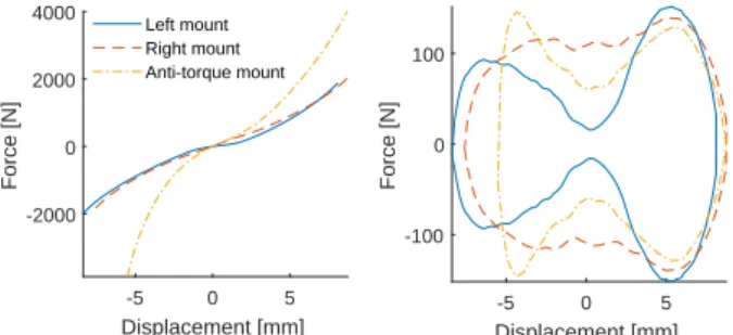
In order to apply the the models on section 2, identifi-cation tests were made on three mounts that compose a powertrain suspension. These tests were made with enforced displacement at constant and low speed, and the results are illustrated by figure 8.
-8 -6 -4 -2 0 2 4 6 8 Displacement [mm] -2000 0 2000 4000 Force [N] Left mount Right mount Anti-torque mount
Figure 8: Force/displacement response for the three tested mounts
The curly shape of test data suggests the presence of a non linear elastic component and classical dis-sipative models are not capable of representing this kind of behavior. A nonlinear elastic model was built using the mean test load for each displacement and is shown in figure 9 left.
The remaining forces, shown in figure 9 right, are supposed to be the generated by the dissipative model in parallel of the nonlinear elastic model. The left mount (and on a smaller scale the anti torque mount) presents significantly less dissipation around null dis-placement. It is probably because a significant part of the rubber is not excited within small displace-ments, and after a certain level, it is solicited by a self-contact.
-5 0 5 Displacement [mm] -2000 0 2000 4000 Force [N] Left mount Right mount Anti-torque mount -5 0 5 Displacement [mm] -100 0 100 Force [N]
Figure 9: Non-linear elastic response (left) and dissipative forces (right) for the tested mounts
Tracing the stiffness as function of distance to the turning point without the nonlinear elastic contribu-tion, in figure 10, as it was suggested in section 2, one can see that its evolution for small distances to the turning point is quite similar to the ones provided by hysteretic models. The absence of dissipation around null displacement creates bumps in the curves be-tween 6 and 10 mm, more visible for the left mount. The end of the curve shows strong negative stiffness, as for a form of symmetry, which is probably due to the removal of a nonlinear elastic part.
2 4 6 8 10 12 14 16 e-e turn [mm] -150 -100 -50 0 50 100 150 K [N/mm]
Left mount loading ( 3) Right mout loading ( 3) Anti torque mount loading
Figure 10: Stiffness in function of the distance to the last turning point without nonlinear elastic component
To fit the dissipation in parallel of the non-linear elasticity, two different models were used: one is the STS model and the other is a simple viscous dissipa-tion. Both models were tuned to dissipate the same amount of energy for a harmonic solicitation with frequency close to the powertrain rolling frequency (around 10 Hz), with the same amplitude as the iden-tification tests. Figure 11 shows the instant dissipation for both models of the right mount under the stated load, and even if the total dissipation is the same, their instant dissipation is different.
4 APPLICATION CASE
With the mounts identified, a model of the whole powertrain suspension was developed. The power-train unit modeled by its mass and inertia matrix, while the three mounts are attached on one side to the powertrain unit, and the other to the chassis, consid-ered as rigid as shown in figure 12. The model input is the engine torque, applied in the direction of the
0 0.02 0.04 0.06 0.08 0.1 Time [s] 0 20 40 60 80 Dissipation [mW] STS Viscous
Figure 11: Instantaneous dissipation for a STS model and a vis-cous model under harmonic solicitation
crankshaft and whose time evolution is illustrated in figure 13, and the outputs are the forces exerted by the three mounts on the body.
Figure 12: Assembled powertrain unit and its suspension
0.4 0.6 0.8 1 1.2 1.4 1.6 Time [s] -600 -400 -200 0 200 400 Torque [Nm]
Figure 13: Measured torque for a starting engine
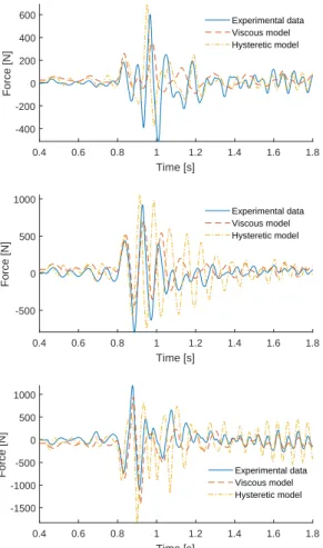
Figure 14 shows the experimental results and sim-ulated forces for both models in the direction of the vehicle motion.
With forces and displacements available for post treatment, viscous dissipation may be explicitly com-puted, and hysteretic dissipation may be computed by equation 2. Figure 15 illustrates the evolution of dissi-pated energy for both computed models, and it high-lights the fact that for this transient simulation, the dissipated energy differs both in total dissipated en-ergy and timing of when the enen-ergy is dissipated. This demonstrate that the original equivalence shown in 3 is not sufficient to provide a proper transient simula-tion.
0.4 0.6 0.8 1 1.2 1.4 1.6 1.8 Time [s] -400 -200 0 200 400 600 Force [N] Experimental data Viscous model Hysteretic model 0.4 0.6 0.8 1 1.2 1.4 1.6 1.8 Time [s] -500 0 500 1000 Force [N] Experimental data Viscous model Hysteretic model 0.4 0.6 0.8 1 1.2 1.4 1.6 1.8 Time [s] -1500 -1000 -500 0 500 1000
Force [N] Experimental data
Viscous model Hysteretic model
Figure 14: Measured and computed forces at the mounts. Top: Left mount; Middle: Right mount; Bottom: Anti-torque mount
0.8 0.9 1 1.1 1.2 Time [s] 0.5 1 1.5 Dissipated Energy [J]
Left mount viscous Right mount viscous Anti-torque mount viscous LM hysteretic RM hysteretic ATM hysteretic
Figure 15: Dissipated energy for each model
To analyze the implications of this difference into the system level, a modal analysis was carried around the resting position of the engine. As expected, the six powertrain modes are three translational modes and three rotational modes, listed in table 1.
Table 1: Powertrain suspension modes
Mode description Frequency Translation perpendicular to vehicle direction 4.00Hz Translation in vehicle direction 6.04Hz Translation in vertical direction 7.13Hz Pitching powertrain 9.18Hz Yawing powertrain 11.66Hz Rolling powertrain 13.38Hz
Modal amplitudes are the decomposition of the displacement on the directions of the eigenvectors (Bianchi, Balmes, Vermot Des Roches, & Bobillot 2010). This decomposition of the displacement
vec-tor q is given by
qj = φjTM {q} (4)
with φ the mass normalized eigenvectors and M the mass matrix, and qj the amplitude associated to the
mode j. The time derivative of those amplitudes yield the modal speeds which are also necessary for com-puting modal energies using
2Ej = ˙q2j + ω 2 jq
2
j (5)
with Ej the energy and ωj the frequency associated to
mode j. This information is useful to know where the energy flows before being dissipated. Modal energy evolution through time is shown in figure 16, for both hysteretic and viscous models.
0.8 0.9 1 1.1 1.2 Time [s] 0 0.05 0.1 0.15 Modal energy [J] Mode 1 Mode 2 Mode 3 Mode 4 Mode 5 Mode 6 0.8 0.9 1 1.1 1.2 Time [s] 0 0.05 0.1 0.15 Modal energy [J] Mode 1 Mode 2 Mode 3 Mode 4 Mode 5 Mode 6
Figure 16: Modal energies for each model. Top: Viscous model; Bottom: Hysteretic model
Modes 4 and 5 take most of the imposed energy on the system, which is natural, since they represent the rotations along the direction of the imposed torque. The different dissipation models impact strongly on how the energy is transmitted to modes, leading to conflicting information of which mode is more im-portant to address.
5 CONCLUSION
This work focused on a specific range of models whose objective is to emulate the rate-independent nonlinear component of rubber mounts behavior. Models of this type used in industry are often iden-tified with full-cycle dissipation equivalence. This equivalence does not take into account all the nec-essary aspects for a predictive transient simulation. To sustain this argument, an application case where a starting powertrain unit was simulated with two sus-pension models that differ only on the dissipation in-stants and the simulations would lead to different de-sign choices.
The need for identification strategies accounting for a conservative nonlinear elastic part, rate-dependent dissipation (viscoelastic) and rate-independent (hys-teretic) dissipation has only been illustrated here and should be an important aspect of future work. For industrial application, evolution of dissipation with non-linear elasticity may also represent an important component of the model for many mounts.
REFERENCES
Bianchi, J. P., E. Balmes, G. Vermot Des Roches, & A. Bobillot (2010). Using modal damping for full model transient anal-ysis. application to pantograph/catenary vibration. In ISMA, pp. 376.
Bourgeteau, B. (2009). Mod´elisation num´erique des articula-tions en caoutchouc de la liaison au sol automobile en simu-lation multi-corps transitoire.
Brokate, M. & J. Sprekels (2012). Hysteresis and phase transi-tions.Springer.
Coveney, V. A. & D. E. Johnson (2000). Rate-dependent mod-eling of a highly filled vulcanizate. Rubber chemistry and technology 73, 565–577.
Segalman, D. J. (2005). A four-parameter iwan model for lap-type joints. Journal of Applied Mechanics 72(5), 752–760. Sj¨oberg, M. (2002). On dynamic properties of rubber isolators.