Science Arts & Métiers (SAM)
is an open access repository that collects the work of Arts et Métiers Institute of
Technology researchers and makes it freely available over the web where possible.
This is an author-deposited version published in: https://sam.ensam.eu
Handle ID: .http://hdl.handle.net/10985/7276
To cite this version :
Duy Hung MAC, Stéphane CLENET, Jean-Claude MIPO - Comparison of two approaches to compute magnetic field in problems with random domains - Science, Measurement & Technology, IET - Vol. 6, n°5, p.331-338 - 2012
COMPARISON OF TWO APPROACHES TO COMPUTE MAGNETIC FIELD IN
PROBLEMS WITH RANDOM DOMAINS
D.H. Mac
1,2, S. Clénet
1, J.C. Mipo
21
L2EP/Art et Métiers Paris Tech, 8 boulevard Louis XIV - 59046 Lille, France
2VALEO-Systèmes Electriques, 2 rue André Boulle - 94000 Créteil, France
[email protected] [email protected]
[email protected] Keywords: Uncertainties, FEM, random domains.
Abstract
Methods are now available to solve numerically electromagnetic problems with uncertain input data (behaviour law or geometry). The stochastic approach consists in modelling uncertain data using random variables. Discontinuities on the magnetic field distribution in the stochastic dimension can arise in a problem with uncertainties on the geometry. The basis functions (polynomial chaos) usually used to approximate the unknown fields in the random dimensions are no longer suited. One possibility proposed in the literature is to introduce additional functions (enrichment function) to tackle the problem of discontinuity. In this paper, we focus on the method of random mappings and we show that in this case the discontinuity are naturally taken into account and that no enrichment function needs to be added.
1
Introduction
In electrical engineering, to predict the behavior of a real device, numerical models based on the solution of the Maxwell equations are widely used. Thanks to the development of powerful computing tools as well as the development of new numerical methods, the numerical models become more and more accurate. The assumption considering that the effects of uncertainties of input data are negligible compared to modelling and numerical errors can be no longer valid. For a prediction close to reality, numerical methods taking into account these uncertainties were proposed [1, 2]. Among these methods, the probabilistic approach where the input and the output of the models are modelled by random variables or fields is widely used. In computational electromagnetics, there are generally three kinds of uncertainties: those on the source terms, those on the material behavior and those on the dimensions of the apparatus under study. In [3, 4, 5, 6, 7, 8, 9], some methods using polynomial chaos expansions were proposed to quantify the effect of uncertainties on the behavior laws on the outputs of the model. For problems with random domains (the dimensions are uncertain), discontinuities can appear on the field distribution in the “random dimension” (stochastic discontinuity). The approximation with a polynomial chaos expansion (classical polynomial chaos) [10] which is well adapted to approximate random variables with a “smooth” probability density function (pdf) is not well suited to approximate random variables with pdf having several local maxima (mode). However, in the case of a stochastic model involving random dimensions, the pdf of the fields at certain positions can exhibit several modes due
to its stochastic discontinuity. In [11], to improve the approximation, additional functions enriching the original basis of the approximation space can be used to take into account these discontinuities (enrichment basis technique).
Another approach to solve a problem with random dimensions consists in using a random mapping that transforms the problem on the original random domain into a problem on a deterministic domain with a modified behavior law (transformation method) [12, 13]. The randomness in this second problem is bore by the behavior law of the material. In this paper, we aim at comparing the approach based on the enrichment basis technique and the approach based on the use of random mappings, especially when the values under interest are local field values. First, we present the problem when the uncertainties are bore by the behavior laws. Several methods have been proposed and compared to solve this type of problem. We present briefly the most popular non intrusive methods with the associated space of approximation - a truncated polynomial chaos expansion. Then, we present the problem with uncertainties on the geometry. Two methods are presented to solve this problem, the transformation method and the enrichment basis method. In the transformation method, the initial problem is transformed into a problem where the uncertainties are bore by the behavior law. In this case, the usual truncated polynomial chaos expansion can be used. Else, if the problem is directly solved (remeshing technique conforming to each geometry realization for example), it is shown that the space of approximation should be enriched to take into account the discontinuity of the magnetic field. The two methods are compared on an analytical example and on a numerical example.
2
Uncertainties on the behavior law
A probabilistic approach can be used to model the uncertainties of an electromagnetic problem. In a stochastic magnetostatic problem with uncertainties on the behavior law, the permeability can be modelled by a random field. We suppose that this random field can be expressed as a function of known random variables ξ (Gaussian variables or uniform variable or…) with a joint probability density function fξξξξ( )ξξξξ . The number of random variables ξ =(ξ1, ξ2 …,
ξd) is equal to d. A stochastic magnetostatic problem defined on domain D with uncertainties on the behavior law can
be written: ( , ) 0 ( , ) 0 ( , ) ( , ) ( , ) B H B H x x x x x = = = ξξξξ ξξξξ ξ µ ξ ξ ξ µ ξ ξ ξ µ ξ ξ ξ µ ξ ξ div curl (1)
where B x( , )ξξξξ the magnetic flux density, H x( , )ξξξξ the magnetic field and µ ξµ ξµ ξµ ξ( , )x the permeability of the domain. For the sake of simplicity, it is assumed that the current density is null in the domain D and that the source term is bore by the boundary conditions defined on the boundary ΓDof D:
D H B B H 0 = 0 B H : ( , ) : ( , ) x x Γ = Γ ∪ Γ Γ ⋅ = Γ × ξξξξ ξξξξ n n (2)
where n represents the unit outward normal vector. The scalar potential formulation is used to solve the system of equations (1) and (2). The scalar potential Ω( , )xξξξξ is defined such that:
( , ) ( , )
H xξξξξ = −gradΩ xξξξξ (3)
The scalar potential is constant on each connected surface of ΓH and we have Ω( , )xξξξξ =0 on ΓH1 and Ω( , )xξξξξ =Von ΓH2. By replacing (3) into (1) we obtain:
( ( , )µ xξξξξ ⋅ Ω( , ))xξξξξ =0
div grad (4)
Regarding the solution of (4), two approaches can be used : the non intrusive and intrusive approaches. The non intrusive approach (Monte Carlo simulation, projection method, regression method…)[5, 14] consists in determining a bunch of appropriate values for the input data then in solving the deterministic model with these series of input data and finally to exploit the values of the output data in a processing step. The non intrusive method consists in adding just an additional “layer” to a deterministic model to take into account the random dimensions. For the intrusive method, a new code has to be developed [3, 4, 6, 7]. The equation (4) can be solved by using the finite element method. In this case, the scalar potential is sought in the nodal shape function space, and we have:
1 ( , ) ( ) ( ) ( ) n i i i x λ x Vβ x = Ω ξξξξ =
∑
Ω ξξξξ + (5)where Ωi( )ξξξξ are random variables to determine, λi( )x , i=1 : n nodal functions of nodes that are not located on
H
Γ and β(x) a linear combination of the nodal function associated to the nodes located on ΓH 2 where the magnetic potential is assumed to be constant and equal to V.
In this paper, we will focus only on some non intrusive methods that are briefly presented in the following part.
3 Non intrusive methods
We will present two non intrusive methods frequently used to solve a stochastic problem: the regression method [5] and the projection method [14]. We are interested in a random quantity G(ξ) (energy, torque, the nodal value of
( )
i
Ω ξξξξ in (5), local value of B, H…). This random quantity is approximated by a polynomial chaos expansion:
1 G( ) G ( ) ( ) P P i i i α = ≈ =
∑
Ψ ξ ξ ξ ξ ξ ξ ξ ξ ξ ξ ξ ξ (6)where Ψi( )ξξξξ are multidimensional orthonormal polynomials [10] andαithe coefficients to determine. Different methods can be used to calculate the coefficients αi.
3.1. Projection method
Due to the fact that the polynomials Ψi( )ξξξξ are orthonormal, coefficients αiare determined by:
[
( ) ( )]
( ) ( ) ( ) d i i i R G G f d α =E ξξξξ ⋅ Ψ ξξξξ =∫
ξξξξ ⋅Ψ ξξξξ ⋅ ξξξξ ξ ξξ ξξ ξξ ξ (7)where E[X] is the expectation of the random variable X. Equation (7) means that the approximation GPis the
projection of G in the functional space S generated by the P polynomials Ψi( )ξξξξ : span( i( ), 1: )
S = Ψ ξξξξ i= P (8)
Different methods can be used to approximate the integral (7): Monte Carlo simulation method, Gauss quadrature method, sparse grid method, adaptive integration scheme [15, 16, 17]... All of them yield the following expression for the approximation: 1 ( ) ( ) N i k k i k k G α ϖ = ≈
∑
⋅ ξξξξ ⋅ Ψ ξξξξ (9)where ϖk are the weights and ξξξξkthe evaluation points. A number of deterministic calculations has to be undertaken to determine G(ξξξξk) for each point ξξξξk k =1 : N. So, the deterministic model has to be solved N times with ξξξξkas input data.
3.2. Regression method
With the regression method, the coefficients αi are determined by minimizing the following criteria [5]:
1 2 2 1 2 ( , ,... ) ( , ,... ) arg PMin( ( ( ) ( )) ) P P P α α α G G α α α = ∈ ξξξξ − ξξξξ R E (10)
Using the orthonormal property of Ψi( )ξξξξ this condition leads also to (7). However, in practice, only a finite number
of evaluations of G( )ξξξξ are available to estimate ( ( )G −GP( ))2
ξξξξ ξξξξ E . Hence:
[
]
1 2 1 2 ( , ,... ) 1 2 ( , ,... ) arg P Min ( ( , ,... )) P P α α α r P α α α = ∈R α α α (11) with 2 1 2 1 1 ( , ,... ) (G( ) ( )) N P P k k i i k k i rα α α ω α = = =∑
ξξξξ −∑
Ψ ξξξξ (12)For the evaluation points ξξξξk, the roots of the polynomial Ψq( )ξξξξ is one possible choice and the weight can be given by 1 /
k N
ω = [18]. The minimization of (12) leads to solve the following linear system:
A⋅ =αααα a (13) with : 1 1 [ ] ( ) ( ) [ ] ( ) G( ) and [ ] with , 1: A N ij k i k j k k N i k i k k k i i i j P ω ω α = = = Ψ Ψ = Ψ = =
∑
∑
ξ ξ ξ ξ ξ ξ ξ ξ ξ ξ ξ ξ ξ ξ ξ ξ αααα a (14)In this method, N evaluations G(ξk), k =1: N are required. The choice of evaluation points ξξξξkand the associated weight
is an issue because a non appropriate choice can lead to a singular system or at least to a ill-conditioned linear system (13).
One can notice that with the same choice of ωk and ξξξξk between (12) and (9) and with N high enough to have an exact
quadrature (so that
1 [ ]A ( ) ( ) N ij k i k j k ij k ω δ =
=
∑
Ψ ξξξξ Ψ ξξξξ = ), the regression method and the projection method give the sameresults.
3.3. Discussion on the polynomial chaos
If ξ is a Gaussian random variable, the Cameron-Martin lemma [19] shows that the approximationG ( )P ξξξξ in (6) tends
to G(ξ) when P tends to infinity (if the variance of G(ξ) exists). In [10, 8], a generalization has been discussed for non Gaussian random variables ξ. However, the convergence rate of (6) depends on the smoothness of G(ξ). When G(ξ) presents some discontinuities with respect to ξ, the convergence rate of (6) can become very slow because the right hand side of (6) is continuous and infinitely differentiable with respect to the components of ξ. In a problem with uncertainties on the behavior law, the electromagnetic field keeps the same discontinuity properties as the random permeability. So if the permeability can be expressed as a polynomial chaos expansion then the polynomial chaos is well fitted to approximate the magnetic field. However, we will see in the following part that in a problem involving uncertainties on the geometry, the magnetic field at a point located close to a random interface can be discontinuous. In this case, a specific treatment has to be introduced to speed up the convergence rate as we will see in the section 4.
4 Uncertainties on the geometry
The uncertainties on the geometry can be modelled by random interfaces Γk between two sub-domains Di and Dj
(purple lines in domain D(ξ) in Fig. 2). In each sub-domain, the behavior law (permeability) is assumed to be homogeneous. We suppose also that these interfaces can be parameterized by known random variables ξ and a parameter c, we have: 1 1 2 2 2 3 3 with ( , ) ( , ) ( , ) k k k k x g c x g c c x g c = = ∈ ∆ ⊂ = ξξξξ ξξξξ ξξξξ R (15)
where x1, x2, and x3 are the coordinates of the points located on this interface. The parameter c belongs to ∆k a subset of
R2 (
Rin 2D case) and g1k, g2k, g3k are known expressions. For each realization of ξ, there is a bijective map between ∆k
and Γk. The permeability µ depends on the position x and also on the realization of the random interfaces. Actually,
for a point x located close to a random interface Γk, the value of the permeability depends on which side of Γk the point x is located. Thus, in a given point x of D which can be located on both sides of a random boundary Γk (between the
subdomains Di and Dj) the permeability switches from the values µµµµi and µµµµj. If we denote IDi (x,ξ), the indicator
function associated to the domain Di (IDi(x,ξ)=1 if x∈Di and 0 elsewhere), the permeability of the domain D can be
written under the form:
0 D 1 I ( , ) ( , ) i n i i x x = =
∑
µ ξ µ ξ µ ξµ ξ µµ ξξ µ ξ µ ξ (16)where n0 is the number of subdomains. Since the permeability is a random field, the magnetic field H and the magnetic
flux density B are also random fields. To deal with the problem with random domains, an easy way consist in using a non-intrusive method with a remeshing step for each evaluation point ξξξξkthat corresponds to a new geometry. However, this approach has some drawbacks. At first, the fact that we have to perform a remeshing, then to restore the stiffness matrix and the source vector for each evaluation point ξξξξkmakes the problem very time consuming. Furthermore, the remeshing of the domain D adds a numerical noise on the output data because mesh (the connectivities between elements, the number of element…) changes from an evaluation point to another [20]. Furthermore, since the mesh changes from an evaluation point to another, the expression of the shape functions changes as well. Consequently, it is not obvious to obtain a simple expression of the distribution of the fields H and B. Finally, as we will see in the following part, the magnetic field at certain fixed points could have some discontinuities in stochastic dimension. Therefore, the approximation of magnetic field at this point by (6) is no longer appropriate. To avoid the former drawback, one possibility is to introduce additional functions (enrichment basis method) that can account for the discontinuities. This technique has been proposed for the stochastic finite element method in [11].
Another possibility consists in using the transformation method proposed in [12, 21]. In the following, a 1D analytical example with random interface will be presented to illustrate the issue of the stochastic discontinuity and to present the principle of both methods listed above.
4.2. Analytical example
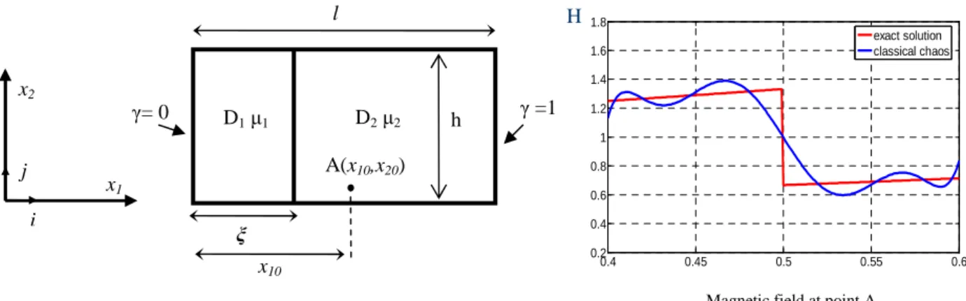
We are interested in a one dimension magnetostatic problem presented in Fig. 1. On two opposite sides of the
rectangular domain D of length l, a magnetomotive force γ0=1 is prescribed. The domain D is split into 2 subdomains
with two different permeabilities µ1 and µ2. The position ξ of the straight interface between the two subdomains is
random. This random interface can be represented by:
1 1 2 2 with 0 ( , ) ; ( , ) x g c c h x g c c = = ∈ = = ξ ξ ξ ξ ξ ξ ξ ξ ξξξξ (17)
We suppose that ξ is a uniform random variable that varies in the interval [0.4.l – 0.6.l]. We focus on a fixed point A with the coordinate x10 within the interval [0.4. l – 0.6. l]. The analytical expression of the component following x1 axis
(other components equal obviously zero) of the magnetic field at this point is given by:
0 1 10 10 2 1 0 2 10 10 2 1 ( , ) with ( ) ( , ) with ( ) H H A A x x l x x l γ µ µ µ γ µ µ µ = < + − = > + − ξ ξ ξξ ξξ ξ ξ ξ ξ ξ ξ ξ ξ ξ ξ ξ ξ ξξ ξξ ξ ξ ξ ξ ξ ξ ξ ξ ξ ξ (18)
We can notice that since the permeabilities µ1 and µ2 are different, the magnetic field at the point A is discontinuous
with respect to ξ at the value ξ = x10 . We seek for an approximation H ( 10, )
P
A x ξξξξ of HA(x10, )ξξξξ under the form (6):
10 10 1 ( , ) ( , ) ( ) H H P P A A i i i x x α = ≈ =
∑
Ψ ξ ξ ξ ξξ ξξ ξξ ξ ξ ξ (19)The coefficients αi have been calculated numerically from (9). The evolution of H ( 10, )
P
A x ξξξξ and HA(x10, )ξξξξ in function of ξ are given in Fig. 1. It shows clearly that the approximation (19) is not appropriate. As expected, the polynomial chaos can not account for the discontinuity of the function HA(x10, )ξξξξ at ξ = x10.
Generally, for a fixed point that can be located in different sub-domains depending on the random interface realization (point A in Fig. 1 can be located in D1 or D2 depending on the value of ξ) the magnetic field is discontinuous at the
stochastic level. The discontinuity appears at the value of ξ for which this point is located on the random interface. For a point that remains in the same subdomains, this kind of discontinuity does not exist and a classical polynomial chaos expansion is well appropriate to approximate the fields. In the following, we will present some methods to deal with this stochastic discontinuity problem. At first, we discuss on the enrichment basis method and then on the transformation method.
4.3. Enrichment basis method
We suppose that the discontinuity point ξ = ξ0 is a priori known. The main idea consists in adding K enrichment
functions into the space of approximation in the stochastic dimension. The approximation (6) becomes:
1 1 ( ) ( ) ( ) ( ) P K P i k i i i i G G + α γ f = = ≈ =
∑
Ψ +∑
⋅ ξ ξ ξ ξ ξξ ξξ ξξ ξξ ξ ξ ξ ξ (20)where fi( )ξξξξ is a discontinuous function at the point ξ = ξ0 and γi the coefficients to determine. The discontinuity of
( )
Gξξξξ can then be taken into account byfi( )ξξξξ . It will speed up the convergence rate of GP+( )ξξξξ towardsG( )ξξξξ (20). A priori, we can use fi( )ξξξξ of the following form:
( ) ( ) ( ) , 1: i i f ξξξξ =τ ξξξξ ⋅ Ψ ξξξξ i= K (21) where: 0 0 1 if ( ) 1 if τ = < − ≥ ξ ξ ξ ξ ξ ξ ξ ξ ξξξξ ξ ξ ξ ξξ ξ ξ ξ (22)
The determination of αi and γi in (20) can be done by either regression method or projection method.
4.3.1. Regression method
Seeking for the stationary point of:
1 2 1 2 1 1 1 ( , ,... ) (G( ) ( ) ( )) N P K P k k i i k i i k k i i Rα α α ω α γ f = = = =
∑
ξξξξ −∑
Ψ ξξξξ −∑
ξξξξ (23)we obtain the following linear system of equations:
A B Bt C = a b αααα γγγγ (24)
where A, B, C are respectively a PxP matrix, PxK matrix and KxK matrix. The vector a is of dimension P and b of dimension K. The coefficients of the previous matrices are given by:
1 1 1 1 1 [ ] ( ) ( ) ; [ ] ( ) ( ) [ ] ( ) ( ) ; [ ] ( ) G( ) [ ] ( ) G( ) ; [ ] and [ ] A B C N N ij k i k j k ij k j k i k k k N N ij k i k j k i k i k k k k N i k i k k i i i i k f f f f ω ω ω ω ω α γ = = = = = = Ψ Ψ = Ψ = = Ψ = = =
∑
∑
∑
∑
∑
ξ ξ ξ ξ ξ ξ ξ ξ ξ ξ ξ ξ ξ ξ ξ ξ ξ ξ ξ ξ ξ ξ ξ ξ ξ ξ ξ ξ ξ ξ ξ ξ ξ ξ α γ ξξ ξξ αα γγ ξ ξ α γ a b (25)In this case, we have to perform N evaluations of G.
4.3.2 Projection method
We seek for the orthogonal projection of G in the space S+:
span( i( ), j( )with 1: , 1: )
which imposes that: 0 with 1 0 with 1 ( ( ) ( )) ( ) : ( ( ) ( )) ( ) : P i P j G G i P G G f j K + + − ⋅ Ψ = = − ⋅ = = ξ ξ ξ ξ ξ ξ ξ ξ ξ ξ ξ ξ ξ ξ ξ ξ ξ ξ ξ ξ ξ ξ ξ ξ E E (27)
Equation (27) leads to a linear system:
E F Ft H = e h αααα γγγγ (28)
where E, F, H are respectively a PxP matrix, PxK matrix and KxK matrix. The vector e is of dimension P and h of dimension K. The vector of the unknown coefficients are α and γ of dimensions P and K respectively. The elements of the previous matrices are given by:
[
]
[
]
[ ] ( ) ( ) ; [ ] ( ) ( ) [ ] ( ) ( ) ; [ ] ( ) ( ) [ ] ( ) ( ) ; [ ] and [ ] E F H ij i j ij ij i j ij i j i i i i i i i i f f f G G f δ α γ = Ψ ⋅ Ψ = = Ψ ⋅ = ⋅ = ⋅ Ψ = ⋅ = = ξ ξ ξ ξ ξ ξ ξ ξ ξ ξ ξ ξ ξ ξ ξ ξ ξ ξ ξ ξ ξ ξ ξ ξ ξ ξ ξ ξ ξ ξ ξ ξ ξ ξ α γ ξ ξ α γ ξ ξ α γ ξ ξ α γ E E E E E e h (29)In (29) the coefficients of the matrixes E, F, and H can be evaluated analytically. However, for the elements of e and h it requires several integral calculations. One can notice that these integral calculations can be done numerically by (9) but in some cases it requires some additional numerical treatments because of the irregularity (discontinuity) of the integrand. In [11], one technique that consists in using a recursive method and dividing the integral domain into several “boxes” is proposed. However, in a high dimension problem (large dimension d of ξ) this integral calculation method can be very time consuming.
4.4. Transformation method
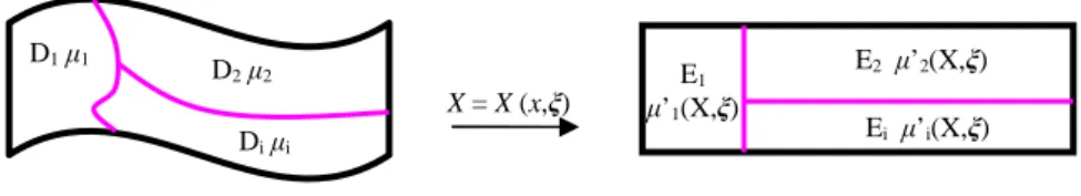
The main idea of this method consists in using a random mapping that transforms the original domain D with random inner interfaces into a deterministic reference domain. The original problem is transformed into a new problem defined on a reference domain E with modified behavior laws that become random fields (Fig. 2).
Actually, the permeabilities on the subdomains of E are not constant anymore but depend on the position and also on the random variables
ξ.
In [12, 21], it is shown that if it exists a one to one random mappingX =X x( , )ξ that transforms the domain D(ξ) into a deterministic domain E, we obtain:
( , )x ′( ( , ), )X x
Ω ξξξξ = Ω ξ ξξ ξξ ξξ ξ (30)
where Ω′is the solution of the scalar potential formulation of the problem defined on the domain E with the modified permeability:
( , ) ( ( , )) ( , ) ( , ) det( ( , )) t M X X x M X X M X µ µ′ ξξξξ = ξξξξ ⋅ ξξξξ ⋅ ξξξξ ξξξξ (31)
withM X( , )ξξξξ the Jacobian matrix of the random mapping. This reference problem, defined on the deterministic domain E with a random permeabilityµ′( , )X ξξξξ can be solved by using the two methods proposed in part 3.1 and 3.2. The magnetic field on the reference domain E can be then approximated by:
1 H( , ) H ( , ) H( ) ( ) P P i i i X X X = ′ ξξξξ ≈ ′ ξξξξ =
∑
′ Ψ ξξξξ (32)From (3) we can deduce an approximation of the magnetic field of the initial problem in D(ξ):
( , ) ( ( , ), ) ( ( , ), )
HP xξξξξ =Mt X x ξ ξξ ξξ ξξ ξ ⋅H′P X xξ ξξ ξξ ξξ ξ (33) We can notice that for a given position X = X0, the Jacobian matrix M(X0, ξ) and H ( 0, )
P
X
′ ξξξξ are continuous with
respect to ξ but discontinuous with respect to X for a given ξ. Therefore, a discontinuity with respect to ξ of ( , )
HP xξξξξ in (33) at some points x=x0 can be taken into account naturally without any enrichment basis technique. In
the transformation method, the main difficulty is the determination of the random mappingX =X x( , )ξξξξ that transforms the original domain D(ξ) to a deterministic reference domain E. In [21] two methods to determine this random mapping were discussed. In the following, we will see with the analytical example presented in part 4.2 how the transformation method enables to deal naturally with the stochastic discontinuity.
4.5 Comparison of both methods on the analytical example 4.5.1. Enrichment basis method
With the enrichment basis method, the magnetic field at point A (Fig. 1) is approximated by:
0 0 1 ( , ) ( , ) ( ) ( ) H H P P A A i i i x + x α α τ+ = ≈ =
∑
Ψ + ξ ξ ξ ξ ξ ξ ξ ξ ξ ξ ξ ξ ξ ξ ξ ξ (34)where τ ξξξξ( )is defined by (22) with ξ0=x10 for this case and αi, α+the coefficient to determine (we use (20) with K=1).
4.5.2. Transformation method
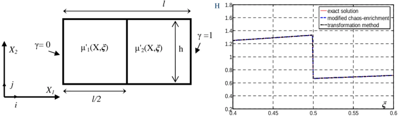
To transform the random domain D(ξ) into a deterministic domain E, one random mapping can be given by the following expression and the corresponding domain E is given in Fig. 3:
1 1 1 1 1 with 2 ( 2 ) with 2( ) 2( ) l x x X l l l x x l l ⋅ ≤ = − ⋅ + > − − ξξξξ ξξξξ ξξξξ ξξξξ ξ ξ ξ ξ ξ ξ ξ ξ (35)
1 1 1 1 2 2 1 1 1 1 2 2 1 ( , ) ' ( ) ' ( ) ( ) ( ) 2 2( ) l l X I X I X I X I X l µ′ =µ +µ = ⋅µ +µ ⋅ − ξξξξ ξ ξ ξ ξ ξ ξ ξ ξ (36)
where I X1( 1)is the indicator function that is equal to 1 when X1 < l/2 and equal zero elsewhere and
2( 1) 1 1( 1)
I X = −I X . The magnetic field in the reference domain is given by the following expression:
0 2 0 1 1 1 1 2 1 2 1 2 1 2 2 ( ) ( , ) ( ) ( ) ( ( )) ( ( )) H X I X l I X l l l l γ µ γ µ ξ µ µ µ µ − ′ = + + − + − ξ ξ ξ ξ ξ ξ ξ ξ ξ ξ ξ ξ ξ ξ ξ ξ ξ ξ ξ ξ ξ ξ ξ ξ (37)
We can notice that the magnetic field in (37) is continuous with respect to ξ when the position X1 is given. Therefore, a
classical polynomial chaos expansion (32) can be used and the magnetic field in the original domain can be obtained by (33).
By using the transformation method, the discontinuity with respect to ξ of the magnetic field still exists naturally in the original domain. Actually, if we focus on the right hand side of (37), the indicator functionsI X1( 1)and I2(X1) that are discontinuous in function of the position X1, do not depend on ξ in the reference domain. By contrast, in the
original domain D(ξ), the functions I X x1( 1( , ))1 ξξξξ and I2(X x1( , ))1 ξξξξ becomes dependant on ξ and since they are discontinuous, the field H is discontinuous. The discontinuities of the magnetic field at some points (point A for example) in the domain D(ξ) with respect to ξ is bore then by these two indicator functions. In Fig. 3, we compare the solution obtained by the transformation method with the one obtained by the enrichment basis method, we can notice that the two methods give very close result to the exact solution (the relative error between solutions and the exact solution is less than 0.2%).
5 Numerical example
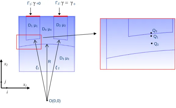
We consider now a magnetostatic problem defined in a random domain D(ξ) presented in Fig. 4. The domain is divided in 4 areas Di, i=1, 4 with relative permeabilities µ1 = µ2 = µ3 =1000 and µ4 = 1. We impose a magnetomotive
force γ = 2A between Γ1 and Γ2 and B.n = 0 on the remaining boundary [22], [23]. The uncertain dimensions (Fig. 4)
are modelled by uniform independent random variables ξ = (ξ1, ξ2) the radius of the two teeth in front of the disk D3.
These uniform random variables are defined in interval [a ; b]. The aim is to compare the magnetic field at the points Q1, Q2, Q3 obtained by a regression method using two methods for the calculation of the evaluation points ξk, denoted
method 1 and method 2. The method 1 is based on the transformation method. The magnetic field is expressed as a classical polynomial chaos expansion. The method 2 consists in remeshing the domain D(ξ) for each evaluation points
ξk. In this case, depending on the location of the point, the magnetic field is approximated either by a classical
The point Q1 is fixed but can be located either in D1 or in D4 depending on the value of ξ1. The point Q2 is fixed also
but located only in domain D4 for every realization of ξ1 and ξ2. The point Q3 is located on the surface of the tooth D1
but remains inside this tooth. This point moves according to the value of ξ1.
We can notice that classical polynomial chaos is well appropriate to approximate the magnetic field at the points Q2
and Q3 due to the fact that these points always remain in the same subdomain for any value of ξ1 and ξ2. The
discontinuity at the stochastic level does not appear for these points. We can notice also that the magnetic fields at the point Q3 that become fixed in the reference domain can be obtained directly by the method 1.
For the point Q1, if the method 1 is used then the discontinuity of the magnetic field is naturally taken into account.
However if the problem is solved directly in the domain D(ξ) (method 2) an enrichment basis method has to be used to improve the approximation.
For the method 1, we use the reference domain with the same form of the original domain but we fix the dimension ξ1
= ξ2= (a+b)/2 (the random mapping is detailed in [21]). The order of the Legendre polynomials for each dimension is
4. The number of polynomial used in (32) is so P = 15. For the enrichment basis technique we use also Legendre
polynomials of order 4 in each dimension and K= P=15 in (20).
TABLE1. Mean value and standard deviation obtained by method 1 and by method 2
Point Q1 Point Q3 Point Q2
Method 1 Method 2 Method 1 Method 2 Method 1 Method 2
Mean-value 1.45 1.47 3.4 x 10⁻³ 3.4 x 10⁻³ 3.12 3.14
Standard deviation 1.49 1.50 2.13 x 10⁻⁴ 2.17 x 10⁻⁴ 0.20 0.20
In Table 1, the mean and the standard deviation of the component following axis x2 (Fig. 4) of the magnetic field
obtained by the method 1 and method 2 are given. The pdf of component following axis x2 of the magnetic field
(estimated using the kernel method) at the points Q1, Q2 and Q3 are given in Fig. 5. We can see that the two methods
give close results. We can notice also that, for the point Q1, the probability density function of the magnetic field has
two modes due to its discontinuity in the stochastic level.
6 Conclusion
We have discussed on the problem with geometric uncertainties. The difference between this problem and the one on the behavior law is that discontinuities in the stochastic dimension can arise. A classical polynomial chaos is no longer suited in this case. One possibility is to use the enrichment basis technique that adds “enrichment” functions in the
space of approximation to take into account this discontinuity. Or we can use the transformation method that leads the problem with geometric uncertainties to a problem with uncertainties on the behaviour law. We have shown that for the transformation method, no enrichment is required. In this paper, the transformation method is applied to a 2D problem. An application in a 3D problem of this method is possible and some numerical methods to determine the random mapping are available in the literature. The transformation method is well fitted for small deformations (to model the effect of the dimension variations in a tolerance interval for example). But, for high deformations, the transformation method can lead to significant numerical errors. In this case, the transformation method should be combined for example with a remeshing method.
References
[1] L. Zadeh. Fuzzy sets as the basis for a theory of possibility. Fuzzy Sets and Systems, (1): 3 - 28, 1978. [2] G. Shafer. A Mathematical Theory of Evidence. Princeton University Press, 1976.
[3] R. Gaignaire, S. Clenet, O. Moreau, and B. Sudret. 3D spectral stochastic finite element method in electromagnetism. IEEE Trans. On Magn. vol.43, no.4, pp. 1209-1212, 2007.
[4] K. Beddek, Y. Le Menach, S. Clenet, O. Moreau. 3D spectral finite element in static electromagnetism using vector potential
formulation. IEEE Trans on Magn Vol.47,pp. 1250-1253, 2011.
[5] M. Berveiller, B. Sudret, M. Lemaire. Stochastic finite element: a non intrusive approach by regression. European journal of computational mechanics. Vol.15, N°1-2-3, pp 81-92. 2005.
[6] R. Ghanem, P.D. Spanos Stochastic Finite Elements: A spectral approach. Dover, New York, 2003
[7] I. Babuska R. Tampone and G.E. Zouraris. Galerkin finite element approximations of stochastic elliptic partial differential equations. SIAM J. NUMER. ANAL.Vol. 42, No. 2, pp. 800–825.
[8] D. Xiu, D. Lucor, C.H. Su, and G. E. Karniadakis. Performance Evaluation of Generalized Polynomial Chaos. P.M.A. Sloot et al. (Eds.): ICCS 2003, LNCS 2660, pp. 346−354, 2003. Springer-Verlag Berlin Heidelberg 2003
[9] E. Rosseel, H. De Gersem, S. Vandewalle. Spectral stochastic simulation of a ferromagnetic cylinder rotating at high speed. IEEE Transactions on Magnetics, volume 47, issue 5, pages 1182-1185, 2011
[10] D. Xiu., G. Karniadakis. The Wiener-Askey polynomial chaos for stochastic differential equations. SIAM J.Sci. Comput 24 (2002) 619-644.
[11] A. Nouy, A. Clément, F. Schoefs, and N. Moes. An extended stochastic finite element method for solving stochastic differential equations on random domains. Comput. Methods Appl. Mech. Engrg. 197 (2008) 4663-4682.
[12] D.H. Mac, S. Clenet, J.C. Mipo, O. Moreau. Solution for static field problem in random domains. IEEE Trans. On Magn, vol.46, no.8, pp. 3385-3388, 2010.
[13] D. Xiu et D.M. Tartakovsky. Numerical methods for differential equations in random domains. SIAM J.SCI COMPUT. No 3, pp.1167-1185, 2006.
[14] Olivier P. Le Maître, Omar M. Knio, Habib N. Najm and Roger G. Ghanem. A Stochastic Projection Method for Fluid Flow. Journal of Computational Physics 173, 481–511 (2001)
[15] Nitin Agarwal and N. R. Aluru. Weighted Smolyak algorithm for solution of stochastic differential equations on non-uniform
probability measures. Int. J. Numer. Meth. Engng 2011; 85:1365–1389
[16] K. Beddek, S. Clénet, O. Moreau, V. Costan, Y. Le Menach, A. Benabou. Adaptive method for Non-Intrusive Spectral Projection –
Application on Eddy Current Non Destructive Testing. Compumag 2011, Sydney, Australia -July 2011.
[17] T. Gerstner, M. Griebel. Numerical integration using sparse grids. Numerical Algorithms, 18 (1998), 209–232
[18] B. Sudret. Uncertainty propagation and sensitivity analysis in mechanical models contribution to structural reliability and stochastic
spectral method. Habilitation à Diriger des Recherches (HDR N°239)-12 October 2007.
[19] R.H. Cameron et W.T. Martin .The orthogonal development of non linear functionals in series of Fourier-Hermite functionals Error
Estimation in a Stochastic Finite Element Method. Annal of mathematics. April 1947.
[20] I. Tsukerman. Accurate Computation of 'Ripple Solutions' on Moving Finite Element Meshes. IEEE Transactions on magnetics. Vol. 31. No. 3, may 1995
[21] D.H. Mac, S. Clenet, J.C. Mipo. Transformation method for static field problem with random domain. IEEE Trans.Magn Vol.47,pp. 1446-1449, 2011.
[22] T. Henneron, Y. Le Menach, F. Piriou, O. Moreau, S. Clenet, J.P Ducreux and J.C. Verite. Source field computation in NDT
applications. IEEE Trans.Magn. vol.43, issue 4, pp. 1785-1788, 2007.
[23] P. Dular, W. Legros and A. Nicolet. Coupling of local and global quantities in various finite element formulations and its application
Fig. 1: Left: magnetostatic problem on domain D(ξ). Right: magnetic field at point A with l =1, µ1=2, µ2=1, P=8 and x10=l/2 ξ D1 µ1 D2 µ2 γ= 0 γ =1 A(x10,x20) x10 x2 i j x1 h l
Magnetic field at point A ξ H 0.4 0.45 0.5 0.55 0.6 0.2 0.4 0.6 0.8 1 1.2 1.4 1.6 1.8 exact solution classical chaos
Fig. 2: Transformation method D1 µ1 D2 µ2 Di µi X = X (x,ξ) E1 µ’1(X,ξ) E2 µ’2(X,ξ) Ei µ’i(X,ξ) Reference domain E Original domain D(ξ)
Fig. 3: Left: problem defined on the reference domain E. Right: magnetic field at point A with P=8 µ'1(X,ξ) µ'2(X,ξ) γ= 0 γ =1 l/2 X2 i j X1 h l 0.4 0.45 0.5 0.55 0.6 0.2 0.4 0.6 0.8 1 1.2 1.4 1.6 1.8 exact solution modified chaos-enrichment transformation method H ξ
Fig. 4. Magnetostatic system Γ1:
γ
=0 Γ2:γ
=
γ
0 O(0,0) R Q1 Q2 Q3 ξ 2 ξ1 D1µ1 D2µ2 D3µ3 D4µ4 x2 i j x1Fig. 5. Probability density function of the magnetic field at the point Q1, Q2, and Q3 0.4 0.45 0.5 0.55 0.6 0.65 0 5 10 15 transformation method remeshing method -2.60 -2.55 -2.5 -2.45 -2.4 -2.35 5 10 15 20 transformation method remeshing method Log(H) Log(H) Point Q3 Point Q2 Point Q1 Log(H) -3 -2.5 -2 -1.5 -1 -0.5 0 0.5 1 0 1 2 3 4 5 6 7 transformation method enrichment technique