Interactions vagues-glace dans l'estuaire et le golfe du Saint-Laurent

UNIVERSITÉ DU QUÉBEC À RIMOUSKI

Interactions vagues-glace dans l’estuaire et le golfe du

Saint-Laurent

Mémoire présenté

dans le cadre du programme de maîtrise en océanographie en vue de l’obtention du grade de maître ès sciences

PAR

© ELIOTT BISMUTH

Composition du jury :

Cédric Chavanne, président du jury, UQAR-ISMER Urs Neumeier, directeur de recherche, UQAR-ISMER Dany Dumont, codirecteur de recherche, UQAR-ISMER

Natacha Bernier, examinatrice externe, Environnement Canada

UNIVERSITÉ DU QUÉBEC À RIMOUSKI Service de la bibliothèque

Avertissement

La diffusion de ce mémoire ou de cette thèse se fait dans le respect des droits de son auteur, qui a signé le formulaire « Autorisation de reproduire et de diffuser un rapport, un

mémoire ou une thèse ». En signant ce formulaire, l’auteur concède à l’Université du

Québec à Rimouski une licence non exclusive d’utilisation et de publication de la totalité ou d’une partie importante de son travail de recherche pour des fins pédagogiques et non commerciales. Plus précisément, l’auteur autorise l’Université du Québec à Rimouski à reproduire, diffuser, prêter, distribuer ou vendre des copies de son travail de recherche à des fins non commerciales sur quelque support que ce soit, y compris l’Internet. Cette licence et cette autorisation n’entraînent pas une renonciation de la part de l’auteur à ses droits moraux ni à ses droits de propriété intellectuelle. Sauf entente contraire, l’auteur conserve la liberté de diffuser et de commercialiser ou non ce travail dont il possède un exemplaire.

Ce que nous accomplissons n’est qu’une goutte dans l’océan. Mais si cette goutte n’existait pas dans l’océan, elle manquerait.

REMERCIEMENTS

Je tiens tout d’abord à remercier mon directeur, Urs Neumeier, pour la confiance qu’il m’a accordée en m’offrant ce projet de maîtrise. C’est grâce à sa rigueur scientifique que j’ai pu mener ce projet de maîtrise à terme, et je lui en suis très reconnaissant. Je le remercie aussi beaucoup de m’avoir donné la chance d’embarquer à bord du Coriolis II à quatre reprises pour des missions scientifiques, ainsi que pour les trois congrès scientifiques auxquels j’ai participé.

Je souhaite également remercier mon co-directeur, Dany Dumont, dont la curiosité scientifique, l’enthousiasme et l’intérêt pour mon travail m’a été d’une précieuse aide dans les moments de doute et m’a permis de garder le moral et la motivation jusqu’au bout. Je le remercie aussi de m’avoir offert un stage avec lui à la Seyne-sur-Mer en France et de m’avoir permis de participer au congrès de l’AGU à San Francisco.

Mes remerciements vont également à Cédric Chavanne et Natacha Bernier pour leur participation à l’évaluation de ce mémoire de maîtrise.

Ce projet de maîtrise a été rendu possible grâce au financement du ministère des Transports du Québec, que je remercie, au même titre que Québec-Océan, qui m’a offert une bourse pour participer au congrès de l’AGU à San Francisco.

J’adresse également une pensée particulière à mes parents, pour leur soutien durant ces trois ans de maîtrise au Québec, à mon père, pour avoir décelé ma passion pour l’océanographie et m’avoir encouragé dans cette voie, et à ma mère pour m’avoir donné le goût de la recherche.

Une pensée aussi pour mes très bons amis Victor et Théo, avec qui l’aventure au Québec a commencé, et sans qui je ne me serais probablement pas rendu jusque-là !

Enfin, je tiens à remercier de tout cœur toutes les formidables personnes que j’ai rencontrées à Rimouski, et qui ont fait de ces trois ans une expérience extraordinaire, autant du point de vue personnel qu’académique. Je ne les citerais pas de peur d’en oublier, mais ils et elles se reconnaitront sans aucun doute : merci les ami(e)s !

RÉSUMÉ

Avec les changements climatiques, le couvert de glace du St-Laurent tend à diminuer, laissant son littoral de plus en plus exposé à l'action des vagues, qui sont le principal facteur d'érosion côtière. La banquise a en effet un rôle protecteur en hiver, puisqu'elle atténue l'énergie des vagues et réduit le fetch disponible pour la génération de vagues par le vent. C’est pourquoi l’évaluation du climat de vagues à long terme dans l’estuaire et le golfe du Saint-Laurent nécessite de prendre en compte la réduction projetée de cette protection par la glace. La première partie de ce mémoire propose une méthode simple pour estimer l’évolution du couvert de glace jusqu’en 2100. Elle est basée sur de nouvelles équations empiriques entre le nombre de degré-jour de gel et les caractéristiques de la saison de glace (début, couverture maximale, durée), qui ont été définies pour le passé récent et qui sont appliquées à un ensemble de simulations climatiques de la température de l’air. L’effet du couvert de glace sur le régime de vagues durant le 21e _{siècle est ensuite estimé en} appliquant aux hauteurs de vagues un coefficient d’atténuation calculé à partir du couvert de glace. Les résultats indiquent une réduction de l’atténuation des vagues d’environ 80% pour la période 2071-2100 par rapport aux trente dernières années (1981-2010). Dans la seconde partie du mémoire, motivé par le désir de mieux représenter les processus physiques en jeu, un modèle spectral unidimensionnel de vagues prenant en compte les interactions vagues-glace et la génération par le vent est développé et utilisé pour étudier les effets de la compétition entre ces processus sur le spectre de vagues. Les résultats montrent que la répartition spatiale de la glace affecte significativement la forme et l’énergie du spectre pour des concentrations partielles entre 20% et 60% de glace.

Mots-clés : climat de vague, glace de mer, interactions vagues-glace, modèle

ABSTRACT

With climate change, the ice cover of the St. Lawrence tends to decrease, leaving its shoreline more exposed to the action of waves, which are the main factor of coastal erosion. Sea ice indeed has a protective role in winter, because it attenuates the wave energy and reduces the distance of open water available for the generation of waves by wind. Therefore, the evaluation of long-term wave climate in the estuary and the gulf of St. Lawrence requires taking into account the projected reduction of the ice protection. The first part of this thesis proposes a simple method to project the evolution of the ice cover until 2100. It is based on new empirical equations between the number of freezing degree-days and the characteristics of the ice season (start, maximum cover, length), which were defined using the recent past and applied on a set of climate simulations of the air temperature. The effect of the ice cover on the wave regime during the 21st century is then estimated by applying on the wave heights an attenuation coefficient computed from the ice cover. Results show a decrease of 80% of wave attenuation for the 2071-2100 period compared to the last thirty years (1981-2010). In the second part of this thesis a one-dimensional spectral wave model that takes into account wave-ice interactions and wave generation by wind is developed and used to study the competition between those processes on the wave spectrum. Results show that the spatial ice distribution significantly affects the shape and the energy of the spectrum for partial ice concentrations between 20% and 60%.

Keywords : wave climate, sea ice, spectral wave model, climate change, Estuary and

TABLE DES MATIÈRES

REMERCIEMENTS ... ix

RÉSUMÉ ... xi

ABSTRACT ... xiii

TABLE DES MATIÈRES ... xv

LISTE DES TABLEAUX ... xix

LISTE DES FIGURES ... xxi

INTRODUCTION GÉNÉRALE ... 1

CHAPITRE 1 MÉTHODE EMPIRIQUE DE PRISE EN COMPTE DE LA GLACE POUR L’ÉVALUATION DU CLIMAT DE VAGUES À LONG TERME DANS LE GOLFE DU ST-LAURENT ... 9

1.1. RÉSUMÉ EN FRANÇAIS DE L'ARTICLE I ... 9

1.2. AN EMPIRICAL METHOD TO TAKE SEA ICE INTO ACCOUNT FOR LONG-TERM WAVE CLIMATE FORECASTING IN THE GULF OF ST. LAWRENCE 10 1.2.1. Abstract ... 10

1.2.2. Introduction ... 10

1.2.3. Methodology ... 13

1.2.3.1. Empirical ice prediction method ... 13

1.2.3.2. Wave attenuation post-processing ... 17

1.2.4. Results ... 19

1.2.4.1. Climate change perturbations on GSL sea ice ... 19

1.2.5. Discussion ... 22

1.2.6. Conclusion ... 26

1.2.7. Acknowledgments ... 27

CHAPITRE 2 MODÉLISATION DE LA GÉNÉRATION PAR LE VENT ET DE L’ATTÉNUATION DES VAGUES EN EAUX COUVERTES DE GLACE : SENSIBILITÉ À LA DISTRIBUTION DE LA GLACE À SOUS-ÉCHELLE ... 29

2.1. RÉSUMÉ EN FRANÇAIS DE L'ARTICLE II ... 29

2.2. MODELLING WIND GENERATION AND ATTENUATION OF WAVES IN ICE-INFESTED WATERS : SENSITIVITY TO THE SUBGRID ICE DISTRIBUTION ... 30

2.2.1. Abstract ... 30 2.2.2. Introduction ... 30 2.2.3. Model description ... 33 2.2.3.1. Advection ... 34 2.2.3.2. Generation by wind ... 34 2.2.3.3. White-capping ... 35 2.2.3.4. Attenuation by ice ... 36 2.2.4. Method ... 36

2.2.5. Results and discussion ... 39

2.2.5.1. Competition between generation and attenuation processes ... 39

2.2.5.2. Sensitivity to the ice distribution ... 41

2.2.5.3. Source of the variability ... 44

2.2.5.4. Illustration of the variability for an idealised case ... 46

2.2.6. Summary and conclusion ... 48

2.2.7. Acknowledgments ... 50

CONCLUSION ... 51

xvii

ANNEXE

LISTE DES TABLEAUX

Table 1. Definition of symbols... 16 Table 2. Results of the regression equations between FDD parameters and ice parameters, with corresponding correlation coefficients R². ... 16 Table 3. Description of model runs used to project the average ice concentration ... 17 Table 4. Fixed default parameters used for WIM ... 39

LISTE DES FIGURES

Figure 1. Ice chart from the Canadian Ice Service (CIS) of the GSL on March 2, 2012. Ice information of the different zones is given by the egg code (Fequet, 2002). The total concentration for this day is 61% in the GSL. ... 11 Figure 2. Schematic diagram of the wave attenuation method. The CIS ice concentration (blue) is approximated by the empirical relations from the FDD parameters (black), to obtain the theorical ice concentration (red dotted line), from which the attenuation coefficient (solid red line) is calculated. The raw wave series (light grey line) is attenuated accordingly (dark grey line). ... 15 Figure 3. Scatter plots of the empirical relationships between FDD parameters and ice parameters for the beginning of winter (left), its duration (middle) and the maximum ice concentration (right). The black stars show the data for the 11 winters (2002 to 2012), and the red line is the correlation curve. The dotted black line is the y = x curve... 16 Figure 4. Wave attenuation calculated from ice concentration, with cmin = 3% and cmax = 60%. ... 18 Figure 5. Evolution of the ice cover. Top. Daily ice concentration averaged on the eight climate simulations. Bottom. Mean (thick line) and standard deviation (color patch) of the ice period (blue, in days) and the maximum ice concentration (green, in %) averaged on the eight climate simulations. The vertical dotted black line shows the start of availability of the 5 CGCM members. Only 4 simulations are taken into account before this line (3 from CRCM and 1 from MERRA) while eight simulations are used after (CRCM and CGCM). The stars represent the data for the 11 winters used to establish the empirical relationships. ... 20 Figure 6. Evolution of the daily attenuation coefficient αn (black curve) and the yearly attenuation coefficient A (thick blue line), for the 3 CRCM simulations used to calculate the wave attenuation. ... 21

Figure 7. Comparison between the ice parameters obtained by the empirical relationships and ROM (Senneville et al., 2013). The Root Mean Square Error (RMSE) is indicated in the top left of each panel. Top : maximum ice concentration for CRCM-aev (unbiased) (left) and CRCM-ahj (right). Bottom : length of ice period for CRCM-aev (unbiased) (left) and CRCM-ahj (right). ... 23 Figure 8. Sensitivity study on the choice of cmax for cmax = 50% (red), cmax = 60% (yellow) and cmax = 75% (blue). Left panel shows the attenuation coefficient calculated from ice concentration. The three right panels show the yearly coefficient

A averaged for the full period (top), the recent past (middle) and the future (bottom),

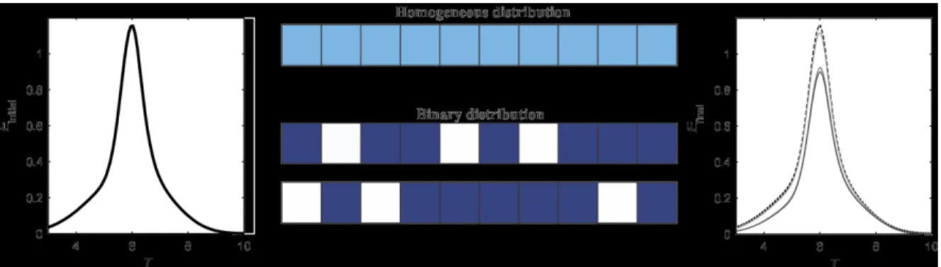
for the three CRCM simulations for each cmax. ... 26 Figure 9. Schema of the two types of ice distributions for fi = 0.3. The initial spectrum Einitial (left) is advected along the ice transect. Depending on the ice distribution (middle), homogeneous (top, fi*= fi in all sub-cells) or binary (bottom, 3 sub-cells with fi*= 1 and 7 sub-cells with fi*= 0), the final spectrum Efinal is different (right, full lines are the three final spectra, the dotted line is Einitial). Only 2 over 120 possible cases are represented for the binary distribution with fi = 0.3 (Figure 10). ... 37 Figure 10. Number of binary transects (N) for each ice concentration (fi). ... 38 Figure 11. Left : evolution of total energy m0 presented as the ratio between final and initial states for a 5-km transect with homogeneous ice concentration from 0 to 1 and constant and stationary wind from 0 to 30 m s-1, for an initial JOSNWAP spectrum with Tp = 6 s and Hs = 1m. Right : same as left panel for the peak energy Ep. ... 40 Figure 12. Top : relative standard deviation (standard deviation standardized by mean value) for m0 (left) and Ep (right) at the end of the 5-km transect for all possible binary transects for ice concentrations between 0 and 1. Bottom : extreme deviation (difference between the maximum and minimum values standardized by the mean value) for m0 (left) and Ep (right). Wind speed varies from 0 to 30 m s-1. ... 43 Figure 13. Evolution of the waves along a 5-km transect with 3 ice distributions, for a total concentration of 0.3 with a 25 m s-1 wind speed. The first panel shows the three different ice transects (homogeneous case in green, the red and blue cases are the binary distributions that lead to the final maximum and minimum energy respectively). The second panel shows the evolution in each sub-cell of m0 (normalized by its initial value), and the two last panels show respectively the wave spectrum and the source term in each sub-cell. ... 45

xxiii

Figure 14. Evolution of wave energy along an idealised 75-km transect. The ice concentration is given at 5-km spatial resolution, and is distributed in three different ways at 500-m resolution (three top panels) with the same colors as in Figure 13. The middle panel shows the final wave spectrum for each case (the dashed black line is the initial spectrum), and the two sub-panels show respectively the wave spectrum at 25 km and 50 km for each case. The bottom panel shows the sum of all the source terms for each case. ... 47

INTRODUCTION GÉNÉRALE

Mise en contexte et problématique du projet de maîtrise

La présence de glace de mer affecte la génération et la propagation des vagues, d’une part en limitant les échanges d’énergie mécanique entre océan et atmosphère, notamment en limitant le fetch (Wadhams, 1983) – distance sur laquelle souffle le vent pour générer des ondes de surface– et d’autre part en atténuant l’énergie des vagues. Les observations pionnières de vagues se propageant dans la glace de Squire et Moore (1980) montrent une décroissance exponentielle de l’énergie des vagues avec la distance et suggèrent que l’atténuation est principalement due à la diffusion élastique causée par les inhomogénéités du couvert de glace (Kohout et al., 2011). En effet, lorsque les vagues changent de milieu de propagation de l’eau à la glace ou de la glace à l’eau, une partie de son énergie est réfléchie, à l’instar d’une onde sonore ou lumineuse. La proportion d’énergie affectée par ce phénomène dépend, pour les vagues, de plusieurs facteurs, notamment leur période et l’épaisseur de la glace, car l’énergie des vagues diminue de manière exponentielle de la surface vers le fond de la colonne d’eau (Holthuijsen, 2007). Les vagues de longue période transportant plus d’énergie que celle de courte période, pour une épaisseur de glace donnée, la proportion d’énergie affectée par le changement de milieu de propagation est plus importante pour les courtes périodes, qui subissent donc une plus forte atténuation. De la même manière, plus la glace est épaisse, plus l’atténuation est importante. Dans le régime linéaire, le nombre d’interfaces eau-glace que les vagues rencontrent dépend donc de la taille des floes de glace ainsi que de leur morphologie. Les phénomènes de dissipation visqueuse (turbulence, déformation inélastiques) peuvent être importants dans certaines situations encore mal définies (Squire et al., 2009). Malgré la difficulté inhérente à la collecte de telles données en milieu naturel, une étude récente basée sur une mission dans la

zone marginal antarctique a mis en évidence que l’atténuation devient plutôt linéaire lorsque les vagues dépassent une certaine hauteur (Kohout et al., 2014). En tout cas, dans un contexte de changements climatiques, la disparition de la banquise laisse présager une intensification du régime de vagues, comme il a déjà été observé en Arctique (Thomson et Rogers, 2014).

Les vagues sont les principales responsables de la fracture de la glace en lui imposant une contrainte de flexion lors de leur passage (Vaughan et Squire, 2011). Lorsque la contrainte exercée par les vagues est supérieure à la contrainte maximale que la glace peut subir, elle se fracture (Squire, 1993). Cette contrainte maximale est extrêmement difficile à évaluer en milieu naturel en raison de la grande inhomogénéité de la banquise. Elle dépend de l’épaisseur de la glace, de ses propriétés mécaniques, qui sont elles-mêmes fonctions de sa salinité et de sa température, et, dans une certaine mesure, de l’historique de déformation (Timco et O’Brien, 1994 ; Langhorne et al., 1998). De plus, la contrainte exercée par les ondes de surface est liée à leurs caractéristiques, comme l’amplitude ou la fréquence ; plus la courbure des vagues est importante, plus la tension exercée sur la glace est importante (Bennetts et al., 2010). La distribution de taille des floes est donc fortement contrôlée par le régime de vagues (Langhorne et al., 1998). Ce mécanisme de fracture de la glace intervient aussi dans les processus de formation et de fonte de la glace en accélérant la fonte latérale des floes en été, ou au contraire en favorisant la formation de glace en hiver par la création d’interstices d’eau libres entre les floes (Steele et al., 1989; Steele, 1992; Bennetts et al., 2010). Kohout et al. (2014) ont d’ailleurs établi une forte corrélation entre la progression ou la récession de la limite de glace et le régime de vagues dans l’océan austral.

L’étude des interactions couplées entre les vagues et la glace de mer est un sujet de recherché très actif actuellement. Cet intérêt est principalement lié à l’accessibilité accrue des régions polaires et le rôle des vagues sur la dynamique de la banquise dans des zones d’intérêt économique important, que ce soit à travers l’exploitation des ressources naturelles (pétrole, gaz, pêcheries) ou la navigation commerciale. Ces activités nécessitent une bonne connaissance de l’environnement polaire, pour garantir à la fois la sécurité des

3

acteurs concernés et la protection du milieu, jusque-là relativement bien préservé de l’influence anthropogénique directe. Par ailleurs, l’effet de rétroaction entre l’intensification du régime de vagues et la fonte de la banquise conduit à une action accrue des vagues sur le littoral, augmentant les risques d’érosion côtière (Overeem et al., 2011).

Dans l’estuaire et le golfe du Saint-Laurent (EGSL), l’érosion côtière est une problématique qui affecte les communautés côtières, et qui pourrait s’aggraver à cause des changements climatiques (Bernatchez et Dubois, 2004; Savard et al., 2009). Les vagues en sont le principal facteur, notamment lors de tempêtes hivernales, dont les effets sont d’autant plus dévastateurs lorsque la banquise n’est pas là pour protéger le littoral en atténuant l’énergie des vagues (Forbes et al., 2004). Afin de prévoir les futurs risques d’érosion côtière, et de proposer des solutions adaptées pour en minimiser les impacts, il est nécessaire de caractériser le climat de vagues de l’EGSL, tâche d’autant plus ardue que la présence de glace en hiver complique considérablement le problème. Étant donné qu’il n’existe pas encore de modèle couplé vagues-glace tenant compte des processus affectant les vagues à la fois en eau libre et dans la glace, l’évaluation du climat de vagues dans le St-Laurent ne tient traditionnellement pas compte de la période hivernale (Ouellet et Drouin, 1991). Cette considération était sûrement valable il y a plusieurs décennies, mais la récente réduction à la fois spatiale et temporelle du couvert de glace saisonnier de l’EGSL en réponse aux changements climatiques (Galbraith et al., 2013; Johnston et al., 2005; Savard

et al., 2009) la rend discutable aujourd’hui.

La caractérisation du climat de vagues dans des eaux saisonnièrement couvertes de glace comme l’EGSL nécessite donc la prévision de l’évolution du couvert de glace. Pour ce faire, des modèles régionaux couplés glace-océan forcés par les solutions de modèles climatiques globaux peuvent être utilisés pour représenter de manière réaliste la dynamique des glaces. Cette méthode a néanmoins un prix élevé en ressources informatiques et restreint le nombre de simulations climatiques que l’on peut réaliser pour évaluer le climat futur de la banquise. Une simulation climatique ne représente en effet qu’une seule réalisation possible du climat, alors que la caractérisation du climat et de son évolution

nécessite plusieurs réalisations. En d’autres termes, plusieurs membres sont nécessaires pour constituer un ensemble représentatif du système climatique. Dans cette optique, une méthode empirique simple basée sur les relations significatives existant entre les principales caractéristiques du couvert de glace et des variables environnementales représente une avenue intéressante pour accomplir cette tâche, pourvu que la corrélation entre les variables soit bonne. Le concept de degrés-jour de gel a été utilisé à maintes reprises pour caractériser la sévérité de l’hiver et les conditions de glace dans les Grands Lacs (Assel, 1980) ou même en Arctique (Lebedev, 1938). Cet indicateur, que l’on définit dans le premier chapitre du mémoire, représente en fait le bilan de chaleur sensible au gré duquel la glace se forme et fond. Il ne tient toutefois pas compte de la dynamique de la banquise, comme le ferait un modèle couplé glace-océan.

La compréhension et la simulation de la complexité des interactions vagues-glace passent nécessairement par l’utilisation de modèles numériques. Plusieurs modèles d’atténuation des vagues par la glace ont vu le jour suite à l’amélioration des connaissances sur les interactions vagues-glace et à l’avancée des méthodes numériques (Kohout et Meylan, 2006, 2008; Squire et al., 2009; Bennetts et Squire, 2012). Ces modèles, basés sur la théorie linéaire de la diffusion des ondes par des plaques élastiques minces flottant dans un fluide non-visqueux incompressible, reproduisent bien les principales caractéristiques de la propagation des vagues dans la zone marginale (Bennetts et al., 2010). Les données disponibles sont pour le moment insuffisantes pour valider ce type de modèle pour l’ensemble des conditions possibles, mais ils représentent à ce jour la meilleure théorie quantitative pour l’étude des interactions vagues-glace. Dans le cadre du projet norvégien WIFAR (Waves-in-Ice Forecasting for Arctic Operators), Dumont et al. (2011) ont proposé le Waves-in-Ice Model (WIM), un modèle qui intègre la théorie de l’atténuation des vagues par la glace et une paramétrisation de la fragmentation des floes afin de prédire la distribution de taille des floes dans la zone marginale à partir de l’information sur les vagues incidentes. Ce modèle donne des résultats qualitativement comparables à ce que l’on retrouve dans le détroit de Fram (Williams et al., 2013b). Il est de plus un outil précieux afin de mieux comprendre et modéliser des processus spécifiques dans une

5

optique d’implémentation des interactions vagues-glace dans des modèles numériques couplés atmosphère-glace-océan, nécessaires pour représenter la globalité des phénomènes physiques influençant la dynamique océanique.

Dans un contexte de changements climatiques, les étendues de banquise des mers du globe tendent à devenir de plus en plus éparses, laissant des étendues d’eau libre disponibles pour l’action du vent, notamment dans la zone marginale de glace arctique, ou dans l’EGSL. Le terme source de génération par le vent a donc été implémenté dans WIM afin de quantifier la compétition entre les processus d’atténuation par la glace et de génération par le vent pour un couvert de glace partiel. De plus, l’amélioration des modèles de vagues implique souvent l’amélioration de la résolution spatiale, notamment pour mieux résoudre les composantes bathymétriques et géographiques (Roland et Ardhuin, 2014). Dans cette optique, la sensibilité de WIM à la résolution spatiale a été explorée en distribuant la glace à fine échelle de différentes manières. Les résultats de cette étude constituent la deuxième partie de ce mémoire.

Ce projet de maîtrise s’inscrit dans le cadre du projet « Modélisation du régime des vagues du golfe et de l’estuaire du Saint-Laurent pour l’adaptation des infrastructures côtières aux changements climatiques » (Neumeier et al., 2013) financé par le ministère des Transports du Québec (MTQ). Il s’inscrit également dans un programme de recherche plus large visant le développement de la prochaine génération des modèles environnementaux couplant atmosphère, vagues, glace et océan, appelés à constituer la base des services de prévisions opérationnels nationaux. Notamment, WIM a été inclut dans la version en développement du code WAVEWATCH III de la National Oceanographic and Atmospheric Administration (NOAA), un modèle qui est utilisé par plusieurs services opérationnels nationaux pour la prévision des vagues.

Objectifs du projet de maîtrise

Le but de ce projet de maîtrise est de quantifier les impacts des interactions vagues-glace dans l’EGSL, afin 1) d’évaluer le climat de vagues et les risques d’érosion côtière dans un contexte de réchauffement climatique et 2) d’améliorer les prévisions de l’état de la mer en présence d’un couvert partiel de glace.

Pour ce faire, les deux objectifs principaux sont :

Objectif 1 : Développer une méthode pour prévoir le climat de vagues hivernal dans l’EGSL jusqu’en 2100.

a) Établir un critère simple permettant de prévoir l’étendue spatiale et temporelle du couvert de glace dans l’EGSL ;

b) Prédire l’évolution du couvert de glace dans l’EGSL jusqu’en 2100 à partir de simulations climatiques ;

c) Évaluer l’atténuation des vagues en fonction du couvert de glace.

Objectif 2 : Améliorer la modélisation des interactions vagues-glace pour un couvert de glace partiel.

a) Implémenter la physique des processus de génération et de dissipation en eau libre dans le modèle WIM (Waves-in-Ice Model ; Williams et al., 2013a, 2013b);

b) Caractériser l’effet de la compétition entre les processus de génération et d’atténuation des vagues dans des conditions de couvert de glace partiel ;

7

Organisation du mémoire et contribution

Chacun des deux objectifs de cette maîtrise a mené à la rédaction d’un article scientifique en anglais. Ces deux articles seront soumis pour publication après le dépôt du mémoire :

L’article 1, An empirical method to take sea ice into account for long-term wave

climate forecasting in the Gulf of St. Lawrence, présente la méthode de prise en compte de

la glace pour l’évaluation du climat de vagues jusqu’à 2100. Une partie de ce travail est aussi intégrée dans le rapport remis au MTQ sur la « Modélisation du régime des vagues du golfe et de l’estuaire du Saint-Laurent pour l’adaptation des infrastructures côtières aux changements climatiques » (Neumeier et al., 2013).

L’article 2, Modeling wind generation and attenuation of waves in ice-infested

waters : sensitivity to the subscale ice distribution, présente les résultats obtenus suite à

l’amélioration du modèle WIM sur la compétition entre génération de vagues par le vent et atténuation par la glace, ainsi que sur la sensibilité de ce modèle à la distribution de la glace à fine échelle.

De plus, ce projet de maîtrise m’a permis de participer à trois congrès scientifiques. Une première affiche, intitulée « Impact du couvert de glace sur le régime de vagues du Saint-Laurent », a été présentée au colloque annuel de Québec-Océan en novembre 2012, présentant les objectifs de la maîtrise. Une deuxième affiche présentant la méthode de prise en compte de la glace a été présentée au colloque de Québec-Océan en novembre 2013 : « Méthode de prise en compte du couvert de glace pour la modélisation du climat de vagues dans le St-Laurent ». Enfin, les résultats préliminaires obtenus avec WIM ont été présentés à l’AGU Fall Meeting à San Francisco en décembre 2013 dans une affiche Intitulée « Modelling wave-ice interactions in the Gulf of St. Lawrence ».

CHAPITRE I

MÉTHODE EMPIRIQUE DE PRISE EN COMPTE DE LA GLACE POUR L’ÉVALUATION DU CLIMAT DE VAGUES À LONG TERME DANS LE

GOLFE DU ST. LAURENT

1.1. RÉSUMÉ EN FRANÇAIS DE L’ARTICLE I

Une méthode empirique permettant d’évaluer l’évolution du couvert de glace et son impact sur le régime de vagues hivernal dans le Golfe du St-Laurent est proposée. Pour cela, les températures de l’air à 2 m de la surface données par le modèle de ré-analyse

Canadian Global Environmental Multiscale (GEM) ont été utilisées pour calculer le

nombre cumulé de degrés-jour de gel. Les cartes de glace du Service Canadien des Glaces ont permis de calculer la couverture de glace journalière des hivers 2001-2002 à 2011-2012. Des relations empiriques ont été établies pour déterminer le début et la durée de la période d’englacement à partir de la température de l’air, ainsi que l’étendue maximale du couvert de glace. Ces relations ont été projetées à l’horizon 2100 grâce à huit (8) simulations climatiques, trois (3) provenant du Modèle Climatique Régional Canadien, et cinq (5) de la 3e génération du Modèle Climatique Global Canadien, afin de déterminer l’étendue spatiale et temporelle du couvert de glace. Un coefficient d’atténuation est ensuite dérivé de la concentration de glace pour être appliqué aux sorties de modèles de vagues. Cette dernière étape constitue une partie du travail de maîtrise de Benoit Ruest, encadré par Urs Neumeier et Dany Dumont.

Cet article a été co-rédigé par moi-même et les professeurs Urs Neumeier et Dany Dumont. En tant que premier auteur, j’ai fait la revue de littérature sur le sujet, le traitement des données de températures et de glace, l’établissement des relations empiriques, et la

rédaction de l’article. L’idée d’utiliser les degré-jours de gel comme critère thermique pour la présence de glace dans l’EGSL provient de Dany Dumont, en s’inspirant des travaux d’Assel (1980) qui a établi un critère de sévérité de l’hiver pour les Grands Lacs à partir du nombre de degré-jours de gel. Urs Neumeier m’a beaucoup aidé dans le traitement des données avec le logiciel Matlab, avec lequel je n’étais alors pas encore très familier. En tant que deuxième et troisième auteurs, Urs Neumeier et Dany Dumont ont activement participé à la direction à prendre pour la recherche et la révision de l’article.

1.2. AN EMPIRICAL METHOD TO TAKE SEA ICE INTO ACCOUNT FOR LONG-TERM WAVE CLIMATE FORECASTING IN THE GULF OF ST.LAWRENCE

1.2.1. Abstract

An empirical method to evaluate the evolution of the ice cover and its impact on the winter wave climate in the Gulf of St. Lawrence is proposed. Air temperatures at 2m above sea level from the Canadian Global Environmental Multiscale (GEM) Model are used to calculate the cumulative number of freezing degree-days. Ice charts from the Canadian Ice Service are used to calculate the daily ice concentration from 2001-2002 to 2011-2012. Empirical relationships are established to determine the start and duration of the ice period, as well as the maximum ice cover. These relationships are projected to the 2100 horizon using eight (8) climate simulations, three (3) from the Canadian Regional Climate Model and five (5) from the 3rd generation of the Canadian Global Climate Model, to determine the spatial and temporal extent of the ice cover. An attenuation coefficient is then derived from the ice concentration to be applied to the outputs of wave climate projections.

1.2.2. Introduction

The Gulf of St. Lawrence (GSL) (Figure 1) is the southernmost seasonally ice-covered basin of the Northern hemisphere and experiences severe coastal erosion, mainly

11

caused by waves, especially during winter storms (Bernatchez and Dubois, 2004; Forbes et

al., 2004). Sea ice acts as a natural protection for the shoreline by reducing the fetch over

which waves can grow (Wadhams, 1983) and by attenuating the wave energy along their propagation in the ice (Squire and Moore, 1980). In a context of climate change, this natural defence forms later and melts earlier in the season, leaving the coast more and more exposed to elements’ wrath.

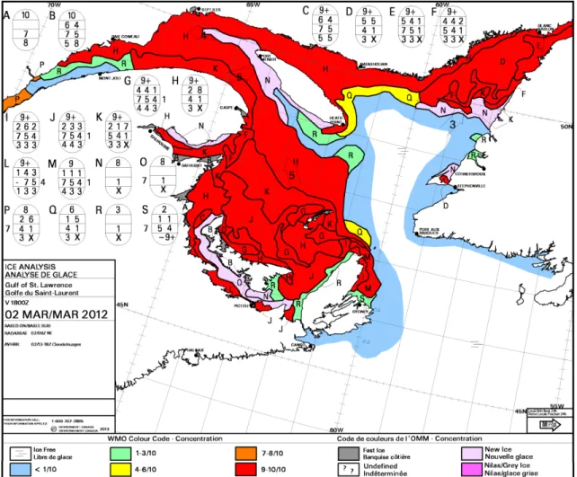
Figure 1. Ice chart from the Canadian Ice Service (CIS) of the GSL on March 2, 2012. Ice information of the different zones is given by the egg code (Fequet, 2002). The total concentration for this day is 61% in the GSL.

Informed management of coastal zones requires either long-term wave data or, when not available, long-term wave model forecasts in order to evaluate the wave climate and the return period of extreme events. This is however not trivial in sub-arctic regions during

winter because little is known about wave-ice interactions. In the GSL, coastal engineers historically did not take into account the winter season for wave climate evaluation (Ouellet and Drouin, 1991), which amounts to consider that waves were fully attenuated by ice. This assumption was perhaps reasonable a few decades ago, but recent observations of the ice season shortening and the maximum ice extent reduction in the GSL as a result of global warming (Galbraith et al., 2013; Johnston et al., 2005; Savard et al., 2009) make it arguable today. Another strategy could be to neglect the effect of ice during winter, which leads to the worst case scenario for coastal erosion risks. These two approaches represent two unlikely extremes of how to take ice into account for long-term wave hindcasting, so a new method between those two is proposed here.

Accurate ice forecasting can be done using regional coupled ice-ocean model simulations forced with Global Climate Model (GCM) solutions, but this comes at a relatively high computational cost mostly due to the need for solving at high resolution (~ 5 km) and the need for relatively high-resolution atmospheric climate simulations (~ 10-50 km) that adequately represent geographical features of the domain. These constraints often lead to reduce the number of simulations, which precludes the characterization of the system’s inherent variability. For these reasons, we propose instead to use simplified empirical relationships based on the concept of freezing degree days (FDD) that capture most of the variability and use them to predict how the ice cover will evolve in the GSL until the 2100 horizon.

Wave attenuation is mainly attributed to ice irregularities that spread and scatter the energy at each wave-ice interface because of the difference in the dispersion relation (Kohout et al., 2011). Furthermore, the attenuation coefficient depends on: the wave period, the shorter ones undergoing more attenuation than the longer ones (Liu and Mollo-Christensen, 1988; Squire, 2007); ice thickness, the thicker the ice the stronger the attenuation; and the floe size distribution, because the number of ice-water interfaces encountered by waves is a determining factor for the amount of energy removed from the waves (Perrie and Hu, 1996; Bennets et al., 2010). However, this kind of wave attenuation modelling requires reliable ice thickness and floe size data that are rarely available from

13

long-term forecasts. A simple and robust method is to apply an attenuation coefficient, derived from the predicted ice concentration, on outputs of models that were run as if no ice were present during winter.

In this paper, we attempt to predict how the sea ice cover will evolve over the next century in the GSL and to evaluate the associated wave climate. Section 2 presents a method to estimate the main characteristics of the ice cover based solely on daily-averaged air temperature data, and a method to associate a wave attenuation coefficient to be used in conjunction with parametric wave models to evaluate the wave climate. Section 3 presents projections of the ice season characteristics for the GSL up to the 2100 horizon and the corresponding impact on wave attenuation. The method is discussed in section 4 and the main conclusions are summarized in section 5.

1.2.3. Methodology

1.2.3.1. Empirical ice prediction method

The concept of freezing degree-days (FDD) has already been used to create a winter severity index and to predict the formation of ice on the Great Lakes (Richards, 1964; Assel, 1980) or other seasonally ice-infested seas (Lebedev, 1938; Rodhe, 1952; Lee and Simpson, 1954). For example, Lebedev (1938) showed that ice thickness is roughly proportional to the square root of the cumulative FDD. Because the GSL is a marine system, the number of freezing degree-days is defined here as the departure of the daily-averaged air surface temperature from the freezing point of sea water, Tf = 1.9°C, where temperatures below (above) Tf are given a positive (negative) algebraic sign. The cumulative number of FDD represents essentially a measure of how cold it has been for how long, and is an indication of the net amount of heat that has been transferred from the ocean to the atmosphere through sensible and latent fluxes over a given period. When it is defined with respect to the freezing point of seawater, it indicates the proportion of heat that contributed to form sea ice. It is calculated at day n as

FDDn = FDDn-1 – (Tn – Tf) × 1 day (1.1a) FDDn = 0 if FDDn < 0 (1.1b)

For the GSL, FDD have been calculated using air temperature 2 m above the sea surface obtained from the Canadian Global Environmental Multiscale (GEM) Model (Côté

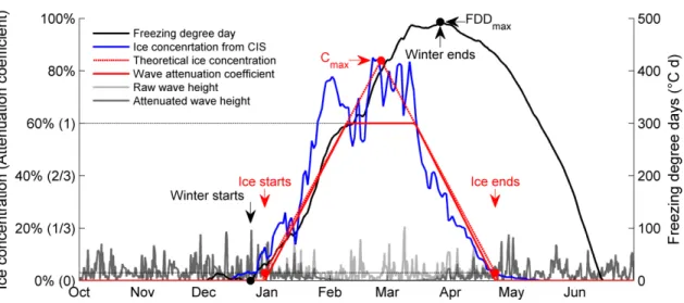
et al. 1998). An example of the time evolution of FDD is shown in Figure 2 (thick black

line). From this curve we define the beginning (the first day FDD is persistently positive) and the end (the day FDD reaches its annual maximum) of winter. Digital ice charts of the Canadian Ice Service (CIS) are used to calculate the average ice concentration c (in %) over the GSL (see Figure 2, thick blue line). Based on this curve, we define the start and the end of the ice season, which are respectively the first days when the ice concentration passes above and below the minimum cmin threshold, and the maximum concentration cmax. With these three quantities we can schematize the ice season as the red triangle shown in Figure 2: the ice concentration increases from cmin to cmax between the beginning and the middle of the ice season, and it decreases from cmax to cmin between the middle to the end of the ice season.

15

Figure 2. Schematic diagram of the wave attenuation method. The CIS ice concentration (blue) is approximated by the empirical relations from the FDD parameters (black), to obtain the theorical ice concentration (red dotted line), from which the attenuation coefficient (solid red line) is calculated. The raw wave series (light grey line) is attenuated accordingly (dark grey line).

The start and the duration of the ice season are respectively related to the start and the duration of winter by linear regressions (Equations (1.2) and (1.3)). The maximum concentration and the maximum of cumulative FDD are linked by a power regression (Equation (1.4)). The symbols used for these parameters are defined in Table 1. Figure 3 shows the correlation curve over the scatter plots of data for the 11 winters (2002 to 2012). Table 2 shows these equations, established for the period of availability of digital ice charts (2002 to 2012), and the corresponding correlation coefficients. The strong correlation between the daily calculated concentration with this procedure and the ice charts data (R² = 0.83) strengthens the reliability of such an empirical method to globally characterize the St-Lawrence annual ice cover. This is not surprising considering the GSL as an almost closed system where the ice freezes and melts locally, even if there is some input from the Arctic Ocean through Belle-Isle Strait and the St. Lawrence River, and some export to the Atlantic Ocean through the Cabot Strait (Hill et al., 2002; Saucier et al., 2003).

Table 1. Definition of symbols.

Symbol [Units] Definition

tfreeze [days] First day when c > 3%

tstart [days] Day when FFD > 0 persistently

tend [days] Day when FDD = FDDmax

lice [days] Duration of ice period

lfdd [days] Duration of winter (lfdd = tend – tstart) FDDmax [°C days]

cmax [%]

Maximum of cumulative FDD Maximum ice concentration

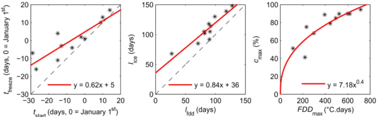
Figure 3. Scatter plots of the empirical relationships between FDD parameters and ice parameters for the beginning of winter (left), its duration (middle) and the maximum ice concentration (right). The black stars show the data for the 11 winters (2002 to 2012), and the red line is the correlation curve. The dotted black line is the y = x curve.

Table 2. Results of the regression equations between freezing degree-days parameters and ice parameters, with corresponding correlation coefficients R².

Equation R2

tfreeze = 0.62tstart + 5 (1.2) 0.78 lice = 0.84lfdd + 36 (1.3) 0.85 cmax = 7.18FDDmax0.4 (1.4) 0.69

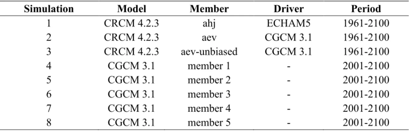
Eight climate simulations produced by two different models, one global and one regional, were used to project the evolution of the average ice concentration in the GSL over the 2001-2100 period using the empirical relationships. All simulations follow the IPCC SRES A2 scenario (Nakicenovic et al., 2000). Five simulations come from the

17

Canadian Global Climate Model (CGCM) 3rd generation and three simulations come from the Canadian Regional Climate Model (CRCM) version 4.2.3 (Table 3). The three regional simulations are called CRCM-ahj, forced by the 3rd member of ECHAM5, CRCM-aev forced by the 5th member of CGCM3.1, and CRCM-aev-unbiased that was unbiased for temperatures using the quantile method (Anandhi et al., 2011) by Senneville et al. (2013). The regional simulations cover the period 1961-2100, but the global simulations only cover the period 2001-2100.

Table 3. Description of climate simulations used to project the average ice concentration.

Simulation Model Member Driver Period

1 CRCM 4.2.3 ahj ECHAM5 1961-2100 2 CRCM 4.2.3 aev CGCM 3.1 1961-2100 3 CRCM 4.2.3 aev-unbiased CGCM 3.1 1961-2100 4 CGCM 3.1 member 1 - 2001-2100 5 CGCM 3.1 member 2 - 2001-2100 6 CGCM 3.1 member 3 - 2001-2100 7 CGCM 3.1 member 4 - 2001-2100 8 CGCM 3.1 member 5 - 2001-2100

The 2-m surface temperatures of the Modern-Era Retrospective Analysis for Research and Applications (MERRA) (Rienecker et al., 2011) are used to define a 30-year reference climate for the period 1981-2010. A second order polynomial correction has been applied to MERRA temperatures to better fit with GEM, which we consider is the best product for air temperatures in the GSL but which is not available over a sufficiently long period.

1.2.3.2. Wave attenuation post-processing

Wave conditions in ice-infested waters result from many processes acting together and affecting their generation, propagation and dissipation. For the purpose of evaluating climatic conditions over a large basin, we continue to adopt a simple parameterization of the effect of sea ice on wave conditions based on the crude fact that the more sea ice there

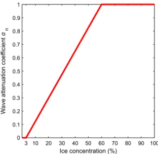
is, the less waves there are. The simplest mathematical representation of this statement is to devise a wave attenuation coefficient  between 0 and 1 that will be applied to the significant wave height determined in the absence of ice. We thus assume that there will be no wave if the ice concentration is above a threshold cmax and that waves won’t be affected if the ice concentration is below cmin = 3%. Between cmin and cmax, we assume a linear function of the daily averaged ice concentration cn. The attenuation αn for day n is then given by

0 if 𝑐n < 𝑐min (1.5a)

𝑐n−𝑐min

𝑐max−𝑐min if 𝑐min <

𝑐

1 if 𝑐_n > 𝑐_max (1.5c)

Figure 4 shows how the attenuation coefficient varies as a function of the averaged ice concentraiton with cmin = 3% and cmax = 60%. A sensitivity analysis of the cmax value is presented in the discussion section.

Figure 4. Wave attenuation calculated from ice concentration, with cmin = 3% and cmax = 60%.

19

The significant wave heights calculated by a wave model have to be multiplied by the attenuation factor (1 − 𝛼n) for the whole ice period. The waves then experience attenuation

proportional to the ice concentration, as it is shown schematically in Figure 2.

Similar approaches are used in wave models that take into account sea ice. In their study for wave forecasting in the seasonally ice covered Baltic Sea, Tuomi et al. (2011) treated the 5-km grid cells of their model in which the ice concentration exceeded 30% as land point. If the ice concentration was lower than this threshold, the cell was considered as open water. Tolman (2003) did the same with a cut-off concentration of 33%. At these values, our parameterization attenuates waves by about half.

1.2.4. Results

1.2.4.1. Climate change perturbations on GSL sea ice

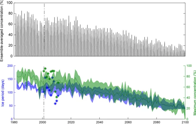
Climate changes affect both the duration of the ice period and the amount of ice formed during winter. Figure 5 shows the ensemble-averaged (eight simulations) ice concentration and the trends of the duration of the ice period and the maximum ice concentration reached yearly. The color patches represent one standard deviation around the mean for the eight simulations for 2001-2100, but only for four simulations for 1981-2001 (three from CRCM and one from MERRA).

All eight climate simulations used to predict the ice cover suggest a substantial shortening of the ice period. The 1981-2010 reference ice climate indicates an average ice period of 112 days whereas the average length for 2071-2100, calculated from the mean of all eight simulations is 65 (±15) days. A decrease of the maximum ice concentration is also predicted by all simulations, from an average of 70.1% for the reference climate to 28.4 (±10.3) % for the average future climate. This represents a loss of approximately 9.8×104 km² for the maximum ice coverage. Furthermore, the 60% threshold for ice concentration, beyond which we consider waves are fully attenuated, won’t be reached anymore after 2059 (±14 years). The last winter when such a concentration is attained is 2077, in

simulation 6. This means there is not a single day after 2077 during which waves are fully attenuated, according to these simulations.

Figure 5. Evolution of the ice cover. Top. Daily ice concentration averaged on the eight climate simulations. Bottom. Mean (thick line) and standard deviation (color patch) of the ice period (blue, in days) and the maximum ice concentration (green, in %) averaged on the eight climate simulations. The vertical dotted black line shows the start of availability of the 5 CGCM members. Only 4 simulations are taken into account before this line (3 from CRCM and 1 from MERRA) while eight simulations are used after (CRCM and CGCM). The stars represent the data for the 11 winters used to establish the empirical relationships.

1.2.4.2. Wave attenuation

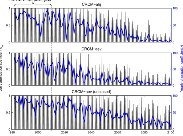
Both the shortening and the decrease of ice cover have consequences on wave attenuation, being less effective and on a shorter period. Figure 6 shows the daily attenuation coefficient calculated from simulations 1, 2 and 3, and the corresponding yearly coefficient A, calculated as the sum of the daily coefficient over the winter:

𝛢 = ∑ 𝛼n n [days] (1.6)

A )

B )

21

The trend of A reflects the evolution of the total impact of ice cover on the seasonal wave climate by taking into account both the ice period and the amount of attenuation. The average yearly coefficient for the MERRA reference ice climate is 64, whereas it is 71 for simulation 1, 63 for simulation 2 and 78for simulation 3 during the same period. These three values respectively fall to 7.1, 6.1 and 21 for the 2071-2100 period, representing a reduction of the total impact of ice of 90%, 90% and 73% respectively, or 84% in mean. This suggests the impact of ice on the wave regime will be four to ten times (six times in mean) less effective in the future period (2071-2100) compared to the recent past (1981-2010).

Figure 6. Evolution of the daily attenuation coefficient αn (black curve) and the yearly attenuation

coefficient A (thick blue line), for the 3 CRCM simulations used to calculate the wave attenuation. Reference climate (recent past)

B ) A ) C )

1.2.5. Discussion

Equations (1.2), (1.3) and (1.4), which link FDDs to the ice cover, bear acceptable physical meaning. Equation (1.2) indicates that tfreeze and tstart are equal on January 14th. Before this date, cold temperatures precede ice formation by the time air cools the water trough sensible heat fluxes, a mechanism that can be slowed by water convection, and by the time water changes state, which is not instantaneous either. After January 14th, some ice appears in the GSL before the winter starts. A plausible explanation for this is that the presence of sea ice in the GSL depends on some level to what happens in adjacent connected water bodies, like the Labrador Sea and the St. Lawrence River. Considering this, it is likely that some inputs of arctic or freshwater ice occur even if the air is not cold enough above the GSL to locally freeze the water. Equation (1.3) indicates that the ice remains in the GSL approximately 30 days longer than the duration of winter. This makes sense knowing that the melting process can be, like the freezing, quite long, depending on ice density and thickness, even if the air temperature is positive. The power regression equation (1.4) is inspired from Lebedev (1938), who linked the ice thickness to the FDD using a power law. This choice ensures that for a null cumulative FDD value, the maximum ice concentration is zero. As we expect the GSL to experience warmer winters in the future, and very few data is available to characterize such winters until now, the utilization of a power regression that converges to zero gives adequate results for ice concentration when the cumulative value of FDDs is small.

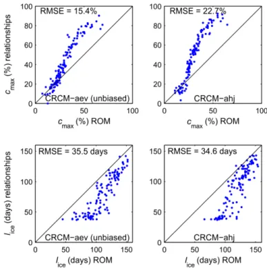
Also these climate relationships assume the stationarity of the ice regime. For example, the ice formation in the GSL is strongly dependent on the Cold Intermediate Layer (CIL), which has experienced erosion these last few years (Galbraith, 2006). One of the shifts in the global GSL mechanisms that could disturb the ice formation is the disappearance of the CIL, in which case such a characterization of the ice climate may no longer be valid. Nevertheless, ice concentration predictions from the FDD empirical method are compared (Figure 7) to the outputs of the Regional Oceanic Model (ROM) with ice formation, dynamic and melting implemented by Senneville et al. (2013) for the GSL.

23

This coupled ocean-atmosphere model has been run only for two CRCM simulations (CRCM-ahj and CRCM-aev (unbiased)), so the validation of the empirical method only concerns these two simulations.

Figure 7. Comparison between the ice parameters obtained by the empirical relationships and ROM (Senneville et al., 2013). The Root Mean Square Error (RMSE) is indicated in the top left of each panel. Top : maximum ice concentration for CRCM-aev (unbiased) (left) and CRCM-ahj (right). Bottom : length of ice period for CRCM-aev (unbiased) (left) and CRCM-ahj (right).

The correlation is quite good for the low values of cmax, and validates the choice of using a power regression to calculate it, even if it overestimates the high values of cmax. This has to be taken into account, but the good correlation for warm winters validates the utilization of the empirical prediction method to characterize the long-term ice climate in a context of global change. However, the ice period is underestimated by the empirical relationships compared to the model, especially for short winters, which is more problematic to characterize the future ice climate in a context of global warming. Nonetheless, the correlation is satisfying with regard to the simplicity of the empirical method. ROM reproduces the thermodynamics processes of sea ice but requires a lot of

computing resources and time, whereas the FDD method gives results quickly and with little computing resources.

The advantage of such a rapidity of execution lies in the large number of atmospheric simulations we can use to predict future ice conditions and the statistically robust wave climate derived from it. Eight simulations have been used to predict ice formation, but only three from the regional CRCM are used to calculate wave attenuation. This choice is a matter of spatial resolution. Because the resolution of the global CGCM (approximately 415 × 280 km at 48°N) is too coarse to adequately represent the wind fields at the scale of the GSL, it should not be used as a forcing of any wave model, whereas the finer resolution of the CRCM (45km × 60km at 48°N) is more adapted for such a purpose. In order to stay consistent, it seems appropriate to use the same atmospheric forcing for both wave and ice forecasting, even if spatial resolution does not affect the average air temperature used for the ice prediction method as much as the wind field used as wave model forcing. This is the reason why only the three CRCM simulations have been used to calculate wave attenuation.

Two assumptions are made for wave attenuation. Firstly, to calculate one daily attenuation coefficient for the whole GSL amounts to consider ice spatial distribution has no effect on wave attenuation. This assumption constitutes the main limitation of the method considering the results of Chapter II of this thesis, which shows that ice spatial distribution can strongly affect wave attenuation in conditions of wind blowing over a partially ice-covered region. Although this assumption simplifies wave behaviour in presence of ice, it is necessary to keep this method simple given the high computational cost and the inaccuracy of long-term climate simulation. Secondly, the same attenuation is applied to all waves regardless to their period, which means the complexity of waves-ice interactions are not taken into account. Nevertheless, ice affects the wave climate in two different ways; the formation of long waves is limited by fetch reduction (Wadhams, 1983), especially in a semi-closed sea like the GSL where waves are locally generated, and short waves are preferentially attenuated when propagating through ice (Liu and

Mollo-25

Christensen, 1988; Squire, 2007). Considering these two processes have an equivalent effect on the energy of short and long waves, it is not so inappropriate to attenuate waves of all periods the same way. Once again, this assumption is made to simplify the method. The alternative would be to use coupled waves-ice models that we consider still not suitable for climate purpose given the actual limited understanding and the difficulty to accurately model waves-ice interactions.

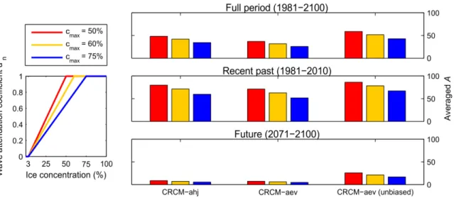
The daily attenuation coefficient is calculated empirically from the average ice concentration in the GSL, in a linear way between 0 if there is less than cmin = 3% and 1 if the concentration is higher than cmax = 60%. The 3% criterion gives the best correlation for equations (1.2) and (1.3). At such concentration, it is very likely that the ice cover will be located very close to the shoreline or at the head of small bays and will not affect waves very much. Figure 1 shows the GSL covered by 61% of ice, and the ice cover appears to be extended enough to prevent the existence of waves along most coastal areas except western Newfoundland. Nonetheless, a sensitivity study was made to quantify the effect of the arbitrary criterion cmax on the averaged yearly attenuation coefficient, with values of cmax = 50% and cmax = 75% (Figure 8). The wave-attenuation variability associated to this parameter is of the same order of magnitude than the variability between simulations. On the other hand, the averaged yearly coefficient A decreases the same from the recent past to the future, independently of cmax. Indeed, this decrease varies between the three cases from 1.3%, 1.1% and 4.8% for simulations 1, 2 and 3 respectively, which means the choice of this parameter has low impact on the reduction of wave attenuation throughout the century.

Figure 8. Sensitivity study on the choice of cmax for cmax = 50% (red), cmax = 60% (yellow) and

cmax = 75% (blue). Left panel shows the attenuation coefficient calculated from ice concentration.

The three right panels show the yearly coefficient A averaged for the full period (top), the recent past (middle) and the future (bottom), for the three CRCM simulations for each cmax.

1.2.6. Conclusion

A simple method to forecast future ice cover in the Gulf of St. Lawrence is presented. Freezing-degree days are used as a proxy to estimate when the ice period starts and ends, and what will be the maximum ice coverage, using air temperature and ice concentration for the last 11 years (from 2002 to 2012). The empirical relationships found to link FDD to ice parameters are projected to the 2100 horizon using 8 climate simulations. The forecasted future ice cover is used to define an attenuation coefficient for wave model outputs, that only take into account the ice concentration, regardless of the wave period or the ice thickness, that are both known to be the most important factors for wave attenuation by ice. Despite the several limitations of this method, it provides a simple method for statistical wave forecasting in seasonally ice-infested waters like the GSL.

The results lead to predict a substantial loss of ice cover throughout the century, with both the maximum ice concentration and duration of ice period being halved by 2100. This means waves will be much less attenuated during winter, by about 80%, leaving the

27

shoreline defenseless facing the winter storms that can already be very destructive. These results match other studies that foresee an increase in coastal erosion risk in Arctic (Overeem, 2011) due to ice cover reduction.

Even if only 3 members have been used to calculate an attenuation coefficient, the interest of such a method lies in the large number of simulations that can be used to predict the ice cover, leading to a statistical estimate of future ice regime. Furthermore, the empirical relationships can be updated every year with new ice and temperature data. This is a simple but interesting alternative to the usual way of forecasting ice cover with resource intensive models.

1.2.7. Acknowledgments

This study was funded by the Government of Québec (Ministère des Transports du Québec). Simon St-Onge-Drouin and Simon Senneville are greatly acknowledged for the outputs of their ice model. We also want to thank James Caveen for his technical support.

CHAPITRE II

MODÉLISATION DE LA GÉNÉRATION PAR LE VENT ET DE L’ATTÉNUATION DES VAGUES EN EAUX COUVERTES DE GLACE :

SENSIBILITÉ À LA DISTRIBUTION DE LA GLACE À SOUS-ÉCHELLE

2.1. RÉSUMÉ EN FRANÇAIS DE L’ARTICLE II

La banquise affecte la génération et la propagation des vagues en réduisant le fetch et en atténuant leur énergie. Dans un contexte de changements climatiques, les couverts de glace deviennent plus épars, laissant de larges bandes d’eau libre disponibles pour l’action du vent. Étant donné que l’atténuation par la glace et la génération par le vent en eau libre sont fortement sélectifs en fréquence et non linéaires, la compétition entre ces deux termes peut mener à des différences significatives dans le spectre des vagues selon la répartition spatiale de la banquise. Pour étudier cette hypothèse, le terme source de génération par le vent a été ajouté à un modèle d’atténuation des vagues par la glace. Cette étude montre que sous certaines conditions, le vent peut générer des vagues au sein d’un couvert de glace partiel. De plus, la sensibilité du modèle à la distribution de la glace à fine échelle a été étudiée, et montre que la compétition entre l’atténuation et la génération est très dépendante de cette distribution.

Cet article a été co-rédigé par moi-même et les professeurs Urs Neumeier et Dany Dumont. En tant que premier auteur, j’ai fait la revue de littérature, l’implémentation et la documentation des processus d’eau libre dans le code du modèle, ainsi que les simulations

faites avec ce modèle. Dany Dumont m’a aidé à me familiariser avec le modèle, qu’il a lui-même développé dans le cadre du projet WIFAR (Dumont et al., 2011), et a donné l’idée originale d’étudier le comportement des vagues pour un couvert de glace partiel en incluant l’effet du vent. Il m’a aussi beaucoup conseillé quant à la direction à suivre pour cette étude. Urs Neumeier a quant à lui aidé à l’optimisation du code du modèle afin de le rendre plus efficace. Tous deux ont aussi participé activement à la révision de l’article.

2.2. MODELLING WIND GENERATION AND ATTENUATION OF WAVES IN ICE-INFESTED WATERS : SENSITIVITY TO THE SUBGRID ICE DISTRIBUTION

2.2.1. Abstract

Sea ice affects the generation and propagation of ocean waves by reducing the fetch and attenuating their energy. In a context of climate change, the ice cover in ice-infested seas becomes sparser, leaving bands of open water free for the wind to blow over. As the competition between the attenuation by ice and the generation by wind in open water has so far received little attention, we explore the implementation of the wind input source term in a waves-in-ice model. This study shows that under certain circumstances, the wind can generate waves inside a partial ice cover. Furthermore, the sensitivity of this model to the subgrid ice distribution is tested, and shows that the competition between attenuation and generation is strongly affected by the way ice is distributed at fine scale.

2.2.2. Introduction

With the climate warming and the ice rapidly decreasing in the Arctic Ocean, new perspectives for commercial activities are envisaged, like oil exploitation and navigation. At the same time, larger ice-free areas also mean that higher seas and swell can be generated. Thomson and Rogers (2014) report that swell of up to 5-m significant height can be generated in the western Arctic when storm winds blow over large ice-free areas open as