Beyond Panel Unit Root Tests: Using
Multiple Testing to Determine the Non
Stationarity Properties of Individual Series in
a Panel
H.R. Moon
yUniversity of Southern California
B. Perron
zUniversité de Montréal, CIREQ, CIRANO
Abstract
Most panel unit root tests are designed to test the joint null hy-pothesis of a unit root for each individual series in a panel. After a rejection, it will often be of interest to identify which series can be deemed to be stationary and which series can be deemed nonsta-tionary. Researchers will sometimes carry out this classi…cation on the basis of n individual (univariate) unit root tests based on some ad hoc signi…cance level. In this paper, we demonstrate how to use the false discovery rate (F DR) in evaluating I(1)=I(0) classi…cations based on individual unit root tests when the size of the cross section (n) and time series (T ) dimensions are large. We report results from a simulation experiment and illustrate the methods on two data sets. Keywords: False discovery rate, Multiple testing, unit root tests, panel data.
JEL classi…cation: C32, C33, C44
We have bene…ted from comments from the guest editors, three referees, and the participants at the conference in honor of Peter Phillips held at Singapore Management University in July 2008 and the CIREQ-CIRANO conference "The Econometrics of Inter-actions" on Oct. 23-24, 2009.
yDepartment of Economics, University of Southern California, Los Angeles, CA 90089,
U.S.A. (213) 740-2108. E-mail: moonr@usc.edu. Financial support from the faculty de-velopment award of USC and the National Science Foundation is gratefully acknowledged.
zDépt. de sciences économiques, Université de Montréal, CIREQ and CIRANO, C.P.
6128, Succ. centre-ville, Montréal, Québec, H3C 3J7, Canada. Tel. (514) 343-2126. E-mail: benoit.perron@umontreal.ca. Financial support from FQRSC, SSHRC, and MITACS is gratefully acknowledged.
1
Introduction
Most panel unit root tests are designed to test the joint null hypothesis of a unit root for each individual series in a panel (see, for example, Breitung and Pesaran (2008) for a recent survey). This raises the issue of how to interpret a rejection of this null hypothesis. It it obviously unwarranted to treat all series in the panel as stationary in this case since this rejection only implies that a signi…cant proportion of the series can be described as stationary. This paper examines how a researcher should proceed in identifying the individual series that can be deemed to be nonstationary and those that can be deemed stationary.
Often, researchers will carry out this classi…cation in empirical work on the basis of n individual (univariate) unit root tests based on some ad hoc signi…cance level. No statistical evaluation of the aggregated decision based on these n individual decisions is provided. To evaluate the aggregation of individual tests, this paper suggests the use of some concepts from the statistical literature on multiple testing. In particular, we will argue that the use of the false discovery rate (F DR) proposed by Benjamini and Hochberg (1995) provides a useful diagnostic on the aggregate decision. The FDR is the expected ratio of the number of falsely rejected null hypotheses over the
total number of rejections. The FDR is interpreted as a posterior of the true null given a rejection of the null hypothesis, (see Storey (2003)).
The main contribution of this paper is to demonstrate how to use the false discovery rate in evaluating I(1)=I(0) classi…cations based on individual unit root tests when he size of the cross section (n) and time series (T ) dimensions are large. We suggest two approaches: the …rst one adjusts the critical value of the individual unit root tests to achieve a targeted FDR level, while the second approach estimates the FDR based on a …xed choice of level for the individual tests (for example, 5%).
Application of F DR as a controlling mechanism for our classi…cation is faced with two di¢ culties. The …rst one is that F DR depends on the (obviously unknown) number of true null hypotheses. Thus F DR is not by itself an identi…ed concept. We solve this problem in our context by the use of the Ng (2008) estimator of the fraction of nonstationary series. The second problem is the presence of cross-sectional dependence among the units in the panel. We solve this problem by applying a bootstrap procedure to estimate the distribution of p-values in the panel and thus control the F DR:
Alternative approaches to classifying the series among I (0) and I (1) components have been proposed. Kapetanios (2003) proposed to carry out a
sequence of panel unit root tests on panels of decreasing size. One removes from the panel the series with the most evidence in favor of stationarity. One continues until the joint test of a unit root for the remaining series in the panel is no longer rejected. On the other hand, Ng (2008) estimates the fraction of nonstationary series. She conjectures that one can then identify the I (1) and I (0) series by ordering them according to the magnitude of their autoregressive parameter.
In independent work, Hanck (2009) uses multiple testing in the context of a mixed panel, but he focuses on the family-wise error rate (F W E), a concept that is less desirable when the number of tests performed (equal to the cross-sectional dimension in this case) is large.
The reminder of this paper is organized as follows: the next section de-scribes the standard panel unit root testing problem, while section 3 presents the multiple testing methodology. Section 4 describes how one can control or estimate the false discovery rate. Section 5 presents simulation evidence that our proposal gives useful information. Section 6 reports results from two empirical applications. Finally, section 7 concludes.
2
Panel unit root testing problem
This section introduces brie‡y the panel unit root testing problem. A more exhaustive review can be found in Breitung and Pesaran (2008).
We suppose that we have panel data zit of individual i that is observed at
time t for i = 1; :::,n and t = 1; :::; T: Hence, n and T denote the size of the cross section and time series dimensions, respectively. We model our panel using a decomposition among deterministic and stochastic components as:
zit = dit+ zit0; (1)
zit0 = izit 10 + yit;
where dit is the deterministic component, and zit0 the stochastic component.
Three basic models of the deterministic components are typically of inter-est: dit = 0 8i; t; dit = i (individual intercepts only), and dit = i + it
(individual trends).
The null hypothesis of interest is that all stochastic components are non-stationary:
whereas the alternative hypothesis takes the form:
HA : i < 1 for some i;
where i is the largest autoregressive root in the time series of individual i: Since a panel unit root test is a joint test, one cannot readily interpret a rejection. In particular, it does not provide any information on the properties of individual time series in the panel. Our goal is to identify the stationary series in the panel and provide a certain statistical evaluation of the identi-…cation based on the individual unit root tests in the panel.
3
Introduction to multiple testing: False
dis-covery rate approach
In this section, we present brie‡y the multiple testing methodology; one can see Lehmann and Romano (2005) for further details.
Suppose that there are n separate testing problems that are either true null or true alternative hypotheses. The number of true null hypotheses will be denoted by n0 and the number of false null hypotheses will be denoted
by n1. The outcome of each test is either to reject or not to reject the null
hypotheses. The testing result can be summarized by the 2 2 table:
# of nulls not rejected # of rejected nulls total
the null is true M0j0 M1j0 n0
the null is false M0j1 M1j1 n1
total n R R n
Thus, R nulls out of n are rejected, and among these R rejections, there are M1j0 false rejections and M1j1 correct rejections.
The familywise error rate is the probability that we incorrectly reject at least one true null hypothesis:
F W E = Pr M1j0 1 :
When looking at a large number of tests, controlling the F W E becomes di¢ cult and requires a decreasing level of individual tests as we increase the number of tests. In such cases, one is often willing to tolerate a few incorrect
rejections. This leads to the k F W E which is the probability that we reject at most k true null hypotheses:
k F W E = Pr M1j0 k
(e:g:; see Lehmann and Romano (2005)).
In panel unit roots, we often look at a panel of increasing size, n ! 1: Thus, for any …xed k; control of the k F W E will encounter similar di¢ culties as control of the simple F W E. It seems natural in this context to let the number of false rejections we are willing to tolerate tend to in…nity and use as our control measure the false discovery proportion, i.e. the proportion of rejections that are false or, using the above notation,
F DP = M1j0
R if R > 0 = 0 if R = 0:
Unfortunately, it is impossible to control this quantity. Instead, Ben-jamini and Hochberg (1995)’s proposal is to control the expectation of the F DP, which they call the false discovery rate (F DR), and which is de…ned
as
F DRP = EP
M1j0
R 1fR > 0g :
Although we will not consider this possibility here, one could also try to control the false non-discovery rate (F N R):
F N R = EP
M0j1
n R1fn R > 0g
which is the proportion of non-rejections that are coming from false null hypotheses or even a weighted average of these two quantities as in Storey (2003).
Storey (2003) provides an interesting Bayesian interpretation of the FDR in the context of a mixture model. Suppose that Hi = 0 (=1) if the ith null
hypothesis is true (or false) and let Hm = (H1; :::; Hm)0: We denote by ^pi
the p-value associated with ith individual unit root test. We know that if
the ith null hypothesis is true, then ^p
i has a uniform distribution on the [0; 1]
interval.
We suppose the random mixture model (^pi; Hi) iid such that
Prf^pi tg = 0U (t) + (1 0) F (t) = G (t) ;
where U (t) = t is the c.d.f. of a uniform distribution and F (t) is the c.d.f. of p-values under the alternative. The variable 0 can be interpreted as the
probability that the null hypothesis is true, in which case the p-values are i:i:d:U [0; 1] :
This result is exact if one uses the exact distribution of the test statistics under both the null and alternative hypotheses. In the case where asymptotic (T ! 1) approximations are used, this result is asymptotic and F (t) ! 1 for any consistent test. In this case,
G (t) = 0t + (1 0) :
For a common size t for all n tests, the number of rejected null hypotheses is: R = n X i=1 1f^pi tg M1j0 = n X i=1 1f^pi tg (1 Hi)
and one can express the false discovery proportion as
F DP (t) =
Pn
i=11f^pi tg (1 Hi)
Pn
i=11f^pi tg + 1 f^pi > tfor all ig
:
where the second term in the denominator avoids division by 0. When the number of tests n is large,
F DP (t)!p 0t
G (t) = E (F DP (t)) (2)
This limit can be re-expressed as:
0t
G (t) =
0U (t)
0U (t) + (1 0) F (t)
= PrfReject the null jHi = 0g P fHi = 0g PrfReject the nullg
= PrfHi = 0j Reject the nullg :
So, the FDR is the posterior probability of the null being true given that we have rejected a particular null hypothesis as the number of tests n ! 1:
4
Control and estimation of the FDR
There are two approaches to using F DR in practice. The …rst one is to adjust the level of individual tests so as to control the resulting F DR: The second approach …xes a level for individual tests and estimates the resulting F DR of this procedure.
4.1
Approaches to control FDR
Benjamini and Hochberg (1995) have suggested to adjust the level of individ-ual tests in the multiple testing procedure to keep the F DR below a level pre-speci…ed by the researcher, . Suppose that the p-values of the n tests have been ordered in ascending order without loss of generality: ^p1 < ^p2 < ::: < ^pn:
They recommend the sequential Hohm method which compares p-values to an increasing critical value. Hypothesis i is rejected if its pvalue is su¢ -ciently small, ^pi ni:They prove that with this method controls the F DR
in the sense that F DR < with probability 1 when this method is used. The BH method of controlling FDR is conservative. It uses the total num-ber of tests in the denominator of the critical values. One can show (Storey et al., 2004) that replacing n by n0, the number of true null hypotheses, would
more hypotheses will be rejected. We will call the FDR-controlling method which rejects null hypotheses when ^pi ni0 the modi…ed BH procedure and
denote it BH :
A di¢ culty with the application of F DR in a panel context is the fact that cross-sectional units display cross-sectional dependence. The above rules have been shown to be valid under independence,although some form of de-pendence can be allowed, see for example. Benjamini and Yuketeli (2001).
As shown by Romano, Shaikh and Wolf (2008) ; the bootstrap or sub-sampling can be used to control for general dependence structures. Their insight is that, for a given set of critical values fc1; :::; cng ; we can
decom-pose F DR as: F DRP = EEP F maxfR; 1gjR = s X r=1 1 rEP [FjR = r] Pr fR = rg = n X r=(n n0)+1 r (n n0) r PrfT1 c1; :::; Tr cr; Tr+1 > cr+1g :(3) We determine critical values to ensure that the above quantity is bounded by the desired F DR level for any probability distribution P: This requires n computations (from least signi…cant to most signi…cant) using up to
n-dimensional integrals and is subject to curse of n-dimensionality.
The bootstrap is used to approximate the joint distribution of the test statistics and calculate the appropriate set of critical values. We need a bootstrap method that allows for serial dependence, cross-sectional depen-dence and non-stationarity. We bootstrap vectors of …rst di¤erences of the data using the moving block bootstrap. Similar methods have been used by Palm, Smeekes, and Urbain (2008) for panel unit root tests and Gonçalves (2009) for a panel regression model. However, Palm et al. (2008) bootstrap residuals from a sequence of individual autoregressions. Hanck (2009) uses a sieve bootstrap on the residuals. One could also use the double resampling of Hounkannounon (2009) which is robust to general forms of cross-sectional and serial correlation.
Our algorithm is as follows:
1. Calculate the …rst di¤erence zit = zit zi;t 1 and collect these as
n-vectors for each time period Zt= ( z1;t; :::; zn;t)0:
2. For a given block size b;draw [T =b] blocks of b consecutive observations of Zt with replacement. Then draw a last block of length T [T =b] b:
3. Generate the bootstrap sample of level variables by cumulating: Zt = t X j=1 Zj:
4. Compute an ADF test for each of the n series in the bootstrap sample.
5. Repeat steps 2-4 B times.
6. Compute the n critical values recursively by solving (3) for n0 = 1; :::; n:
7. Having determined the set of critical values, f^c1; :::; ^cng ; test null
hy-potheses sequentially. Reject the most signi…cant null hypothesis (the one with the smallest statistic) if the ADF statistic for that series is less than c1: If it is, reject the second null hypothesis if T2 < ^c2 and so on
until a null hypothesis is no longer rejected, call it j . The resulting set of I(1) series are those from j to n; and the I (0) series are 1; :::; j 1:
There are three practical di¢ culties with this approach: …rstly, it requires the choice of block size b: As in Gonçalves (2009) ; we set it equal to choice of bandwidth for long-variance estimation in Andrews (1991) : Secondly, as opposed to the other methods described here which are based on individual p-values, the bootstrap method can only be applied to balanced panels. If the
number of cross-sectional units varies over time, the above algorithm would create "holes" in our bootstrap sample. Finally, the method requires the computation of the joint distribution of the n ADF statistics. It is therefore subject to the curse of dimensionality in two ways. Firstly, the accuracy of any estimate of a high-dimensional distribution is likely dubious, even with a large number of bootstrap replications. Second, because we have to compute n critical values, the di¢ culty of computations increases with n: In the simulation experiments below, we do not consider choices of n larger than 30 for that reason.
4.2
Approaches to estimate FDR
Suppose that we …x the level of the individual tests to some quantity : Remember FDR in the limit (as the number of tests gets large) is given by (2) :
F DR = 0
Pr (reject H0i)
:
The natural estimator of this quantity involves replacing 0 and the
looking at the fraction of rejections: \ Pr (reject H0i) = 1 n n X i=1 1(^pi;T ) = R n:
We now derive its limit under sequential asymptotics as T ! 1 followed by n ! 1: 1 n n X i=1 1(^pi;T ) = 1 n n X i=1 1(^pi;T ) Hi+ 1 n n X i=1 1(^pi;T ) (1 Hi) T !1 ! n1 n X i=1 Hi+ 1 n n X i=1 1(Ui ) (1 Hi) n!1 ! (1 0) + 0: (4)
This sequential limit is also joint if the individual unit root tests’s weak limit is uniform in i under both the null and the alternative hypotheses.
Finding an estimator of 0 is more problematic. The fraction of true null
hypotheses is partly the problem we are trying to solve.
In the existing literature, Storey et al. (2004) have proposed the following general estimator:
^0( ) =
1 1nPni=11(^pi )
(1 )
for some 2 (0; 1) : This comes from the fact that large p-values are likely to come from true null hypotheses. Thus, we should expect 0(1 )p-values
above . Asymptotically, this estimator is consistent. To see this, the above estimator is:
^0( ) =
1 n1 Pni=11(^pi )
(1 )
! 1 ((1(1 0) +) 0) = 0:
where the second line follows from (4) : However, Storey et al. proved that this estimator is conservative in …nite samples.
The above estimator depends on a tuning parameter : Storey et al. (2004) provide a data-dependent choice of that minimize mean square error (MSE).
Instead of relying on the above generic estimator, one can, in the context of panel unit root tests, estimate the proportion of true null hypotheses by using the results in Ng (2008). She estimates the fraction of units in a panel that have a unit root by looking at the behavior of the cross-sectional
variance as a function of time: Her key insight is that the cross-sectional variance grows linearly over time with a slope equal to the fraction of the units that are non-stationary.
Ng showed that the cross-sectional variance Vt = n1
Pn
i=1(zit zt)2 is
approximately linear in t with coe¢ cient 0 :
Vtt c + 0t
for some constant c, which suggests the estimator:
^0 = T
X
t=1
Vt:
Ng shows that this estimator converges at ratepn and is asymptotically normal. The estimator is robust to some forms of cross-sectional dependence and one can control for serial correlation by …rst correcting the scale by estimating an AR process.
With estimates of 0 and R; we can get an estimate of F DR as:
\ F DR = ^0 ^ R=n = ^0 1 n Pn i=11(^pi ) ;
which, following the above discussion, is consistent if ^0 p
! 0 and the
de-nominator converges to (1 0) + 0.
5
Simulation
In this section, we report results from a small simulation experiment. We want to analyze the e¤ects on the FDR of the fraction of series with a unit root, the size of n and T; and the extent of cross-sectional dependence.
We …rst ignore the issue of cross–sectional dependence and consider the basic dynamic panel data model (1) with heterogenous intercepts:
zit = i + zit0;
zit0 = izit 10 + uit;
where uit is ARMA(1,1):
(1 L) uit = (1 + L) "it
and "it s i:i:d:N (0; 1) : The autoregressive parameter i is 1 for the …rst 0
We consider 3 values for 0 : .1, .5 and .9. The individual e¤ects i are
N (0; 1) : Finally, we consider three values for each of and ; -.5, 0, and .5 but do not consider cases where the roots cancel each other out. This means that we have a total of 7 pairs of and :
We consider the n null hypotheses that each series has a unit root. We use an ADF test for this purpose. We choose the degree of augmentation in the regression with the MAIC or Ng and Perron (2001) with a maximum of 4 lags. We consider two choices of n and T; n = 10; 30 and T = 100; 500: We do not consider larger choices of n because of the heavy computational burden imposed by the bootstrap procedure of Romano et al. (2008) : We run each experiment 1000 times.
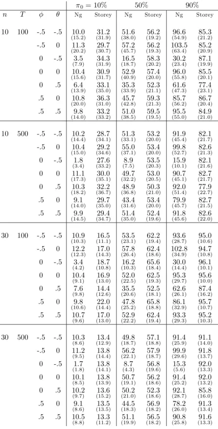
To begin with, we report 2 estimates of 0:Because F DR depends on this
(unknown) parameter, many properties of the F DR estimators and F DR control methods are directly related to these. The …rst estimator is the Ng (2008)estimator A, while the other is Storey’s estimator with data-dependent choice of : The means and standard deviations over the replications are reported in table 1.
Two main conclusions arise from these results. The …rst one is that Ng’s estimator is much less biased than Storey’s which can be quite conservative. However, it has much higher variance which increases with 0: Second, the
Ng estimator is severely biased downward with a negative MA component. This is expected as the I (1) series approach stationary behavior. Unit root tests have been widely documented to su¤er from severe size distortions in this case for the same reason (see Schwert, 1989). There is also a downward bias for the positive MA case for the smaller choice of T (100) ; but this disappears when T = 500: A larger T also makes the Storey estimator less conservative. The size of n does not make any di¤erence on the centering of the Ng estimator, but it reduces its variances (since its rate of convergence is p
n). Increasing n is detrimental to the Storey estimator for 0 = 10%; but
bene…cial for the other values.
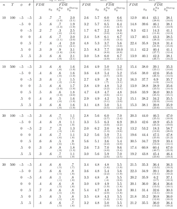
In Table 2, we report the average FDP over the replications (which ap-proaches F DR as the number of replication increases) for a …xed test size of 5% and three (conservative) estimates that di¤er according to the choice of ^0: The …rst one uses the true 0 (and is therefore infeasible), the second
uses Ng’s estimator, and the last one uses Storey’s estimator: We report both the mean and standard deviation of the last two estimators.
*** Insert table 2 here ***
From this table, we notice that F DR increases with 0:That is, if most
series are nonstationary, then …ndings of stationarity are more likely to be false. It also increases with both n and T: Second, the F DR estimators can be quite conservative, particularly for the larger choice of 0: There is
also not much e¤ect of either n or T on the estimators. Finally, the relative performance of these estimators follows that of the estimators of 0:Because
Ng’s estimator of 0 is less biased but more volatile, the estimator of F DR
based on it is less biased but more variable in general. However, it behaves quite poorly in the large MA cases.
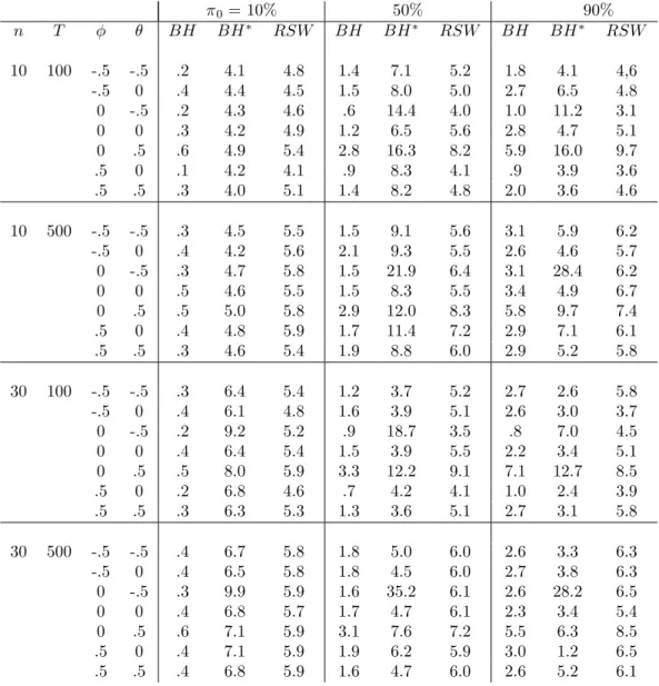
In table 3, we change our approach and report results when we try to con-trol the FDR at 5%. We consider three methods described above. The …rst one is the original Benjamini and Hochberg (BH) method that compares the p-values to an increasing sequence of critical values. This method implicitly assumes that all null hypotheses are correct ( 0 = 1). The second method
is the modi…ed BH method (denoted BH ) which uses the Ng estimator of
0 when calculating the increasing critical values. Finally, we report the
bootstrap-based method of Romano et al. (2008) implemented as described above. If the methods controlled the FDR perfectly, we would expect 5%
in all cells in the table. Numbers below 5% indicate that the method con-trols the F DR since the proportion of false rejections is less than the desired level of 5%. However, it lacks power since we could have rejected other null hypotheses without violating the F DR constraint.
*** Insert table 3 here ***
The …rst thing to note from the table is that the original BH method is very conservative. Despite a desired level of 5%, we reject much less often than that. One thing to note however is that this conservativeness is especially present for the small values of 0: For 0 = :9; the procedure is
not that much conservative. This is due to the fact that BH assumes that
0 = 1 when constructing the critical values. On the other hand, using the
Ng estimator of 0 alleviates these problems as expected. However, in the
cases with large MA components, the F DR is not controlled at all and the method performs quite poorly. Finally, the bootstrap method of Romano et al. performs really well in obtaining an FDR of approximately 5% even in the large MA cases were the modi…ed BH procedure performs poorly.
5.1
Cross-sectional dependence
Our second set of experiments adds cross-sectional dependence through a factor model. The common factor ft is introduced in the residuals as in
Moon and Perron (2004) and Pesaran (2007) :
zit = i+ zit0;
zit0 = izit 10 + yit;
yit = ift+ uit
where the factor loadings are U [0; 1] and the factor is an AR(1):
ft= :5ft 1+ vt
where vt s i:i:d:N (0; 1) . The rest of the design is as above (in particular,
uit is an ARMA(1,1) process with parameters and ).
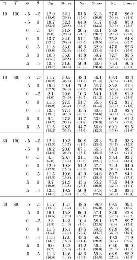
Table 4 reports the results of the estimation of 0 as in table 1 above.
*** Insert table 4 here ***
now overestimates 0 with a large negative AR process. The negative MA
case again leads to a severe downward bias.
Table 5 presents the average proportion of rejections that are false and the same three estimators of the F DR as in table 2 above. First, note that the false discovery rate is lower in this case than in the independent case. This is the usual …nding when there is dependence among the tests under consideration. On the other hand, the estimators of F DR are roughly the same as before, thus leading to a larger bias than before.
*** Insert table 5 here ***
In table 6, we look at the performance of the BH, BH and RSW pro-cedures in controlling the F DR: As expected, the presence of dependence increases the degree of conservativeness of the BH procedure. The BH pro-cedure works quite well except in the large MA cases where the Ng estimator of 0 is severely biased. The bootstrap-based procedure of RSW on the other
hand provides very good F DR control for all parameter con…gurations.
6
Empirical examples
In this section, we employ our proposed approach to classify series in two panels into I (0) and ((1) series.
Our …rst example uses real income data for households from the PSID. We follow Meghir and Pistaferi (2004) and remove households with female heads, with missing education data, and with outliers. We are left with n = 154 households for T = 26 years (1968-1993). As in Ng (2008) ; data is …rst regressed on individual e¤ect, age, age2 and education.
Our second empirical illustration uses exchange rate data. We use the long annual data on real exchange rates relative to the US dollar from Taylor (2002) : 1 Because we require a balanced panel in the application of the
bootstrap to control the false discovery rate, we restrict the sample to the 19 countries for which data is available over the period 1892-1996. Our panel dimensions are thus n = 19 and T = 105: We only allow for a constant term in the deterministics, but our results are similar with the inclusion of a linear trend. Hanck (2009) uses similar data. He mentions that the di¤erences between his results and those of Taylor (2002) are due to di¤erent sample periods, di¤erent intrapolation methods for missing wartime data,
and di¤erent lag length selection. Overall, our individual results are closer to those of Taylor because we only di¤er by small changes in sample period in order to balance the panel and lag selection rules. As reported by Lopez et al. (2005), the results using this data set are very sensitive to the choice of lag length. Using the same lag lengths as those reported in Taylor gives very close results.
The results of the application of our suggested procedures are presented in table 7. In order to increase the power of the unit root tests, we also report results with the application of the DF-GLS test of Elliott el al. (1996) ; and these results are presented in the second column of the table next to those based on ADF tests.
6.1
PSID data
Our estimate of the fraction of households with nonstationary income is about 20% and does not depend on which test is used.
On the other hand, since Storey’s estimator of the fraction of true null hypotheses depends on the p-values of the test, it depends on the choice of test. For the ADF test the estimate is very high, 87%. With the use of the DF-GLS test, the estimate is 27% which is close to the one obtained using
Ng’s estimator.
Turning now to the results of individual ADF tests, with a …xed level of = 5%; we reject the unit root for 24 out of 154 households (or about 16%). The two estimates of F DR re‡ect the large di¤erence in the estimate of 0: The estimator using the Ng estimator is 6.5%, and the one using the
Storey estimator is about 28%. These can be interpreted as the posterior probability that each of these 24 rejections is for a null hypothesis that is false.
Control of F DR at the level of 5% leaves only 9 rejections with the Hohm criterion (the BH method). Use of the bootstrap to allow for dependence leaves a very small number of rejections (2). This result is robust to the choice of block size. It is probably due to the time dimension of the data not being su¢ cient for the application of the block bootstrap.
Results based on the more powerful DF-GLS test are very similar. With a …xed 5% level, we reject the unit root for 25 out of 154 series (instead of 24). The Storey estimator is however much lower than before and close to the Ng estimate. Thus, the FDR estimates are close to one another and quite small, and we can be fairly con…dent that those series that have been classi…ed as I (0) are indeed stationary.
*** Insert table 7 here ***
6.2
Real exchange rates
For the real exchange rate panel, Ng’s (2008) estimate of 0 is negative. This
is the same result that she reports in her paper. Storey’s estimator is 21% with the ADF test and 10.5% with the DF-GLS test. Both estimates suggest a large proportion of stationary series which is rather unusual in tests of PPP. Table 8 provides detailed results for this application.
If we …x the level of tests at 5%, we reject the unit root for 6 countries using the ADF test and 11 for the DF-GLS test. The identity of these countries can be found by looking at table 8. Countries for which we reject the unit root are identi…ed with an asterisk in that table under the heading "5%". The estimate of FDR using Ng’s estimator is negative given the negative estimate of 0, but Storey’s estimator is small. Again, we can have reasonable
con…dence that the rejections are from false null hypotheses.
Controlling for multiplicity using either the Hohm criterion or the boot-strap (the results are identical) leaves a single signi…cant country (Finland) using the ADF test and 10 out 11 using the DF-GLS test (only Denmark drops out).
7
Conclusion
In this paper, we demonstrate how to use the F DR in evaluating I(1)=I(0) classi…cations based on individual unit root tests. In the literature, most of the analysis of the F DR have been done under independence. Yet, in many interesting applications, cross-sectional data are not independent, and sometimes this dependence is quite strong. We illustrate the methods on two panel data sets and use F DR to measure the probability our con…dence in the …ndings of stationarity.
As developed here, the methods used to control or dependence require the use of the joint distribution of the test statistics. To obtain an estimate of this distribution, we rely on the bootstrap, and this method is subject to the curse of dimensionality. Application to panels with a large number of cross-sections would probably require the use of a parametric model of dependence such as a factor or spatial model.
References
[1] Andrews, D. (1991): Heteroskedasticity and Autocorrelation Consistent Covariance Matrix Estimation, Econometrica, 59, 817–858.
[2] Bai, J. and S. Ng (2004): A PANIC Attack on Unit Roots and Cointe-gration, Econometrica, 72, 1127-1177.
[3] Benjamini, Y. and Hochberg, Y. (1995):. Controlling the false discovery rate: a practical and powerful approach to multiple testing, Journal of the Royal Statistical Society, Series B, 57, 289-300.
[4] Benjamini, Y. and Yekutieli, (2001): The Control of the False Discovery Rate in Multiple Testing under Dependency, The Annals of Statistics, 29, 1165-1188.
[5] Breitung, J. and M. H, Pesaran (2008): Unit Roots and Cointegration in Panels, in Matyas, L. and P. Sevestre (eds.), The Econometrics of Panel Data (Third Edition), Kluwer Academic Publishers, 279-322.
[6] Elliott, G. T. Rothenberg, and J. Stock (1996): E¢ cient Tests for an Autoregressive Unit Root, Econometrica, 64, 813–836.
[7] Gonçalves, S. (2009): The Moving Blocks Bootstrap for Panel Linear Regression Models with Individual Fixed E¤ects, mimeo, Université de Montréal.
[8] Hanck, C. (2009): For Which Countries did PPP hold? A Multiple Testing Approach, Empirical Economics 37, 93-103.
[9] Hounkannounon, B. (2009): Bootstrap for Panel Regression Models with Random E¤ects, Mimeo, Université de Montréal.
[10] Kapetanios, G. (2003): Determining the Stationarity Properties of In-dividual Series in Panel Datasets, Working paper 495, Department of Economics, Queen Mary, University of London.
[11] Lehmann, E.L. and J.P. Romano (2005): Testing Statistical Hypotheses, 3rd Ed. Springer.
[12] Lopez, C., C.J. Murray, and D. H. Papell (2005): State of the Art Unit Root Tests and Purchasing Power Parity, Journal of Money, Credit, and Banking, 37, 361-369.
[13] Moon, H.R. and B. Perron (2004): Testing for a Unit Root in Panels with Dynamic Factors, Journal of EconometricsR; 122, 81-126.
[14] Moon, H. R. and B. Perron (2007): An Empirical Analysis of Nonsta-tionarity in a Panel of Interest Rates with Factors, Journal of Applied Econometrics, 22, 383-400.
[15] Ng, S. (2008): A Simple Test for Non-Stationarity in Mixed Panels, Journal of Business and Economic Statistics , 26, 113-127
[16] Ng, S. and P. Perron (2001): Lag Length Selection and the Construction of Unit Root Tests with Good Size and Power, Econometrica, 69, 1519-1554.
[17] Palm, F.C., S. Smeekes, and J.-P. Urbain (2008): Cross-Sectional De-pendence Robust Block Bootstrap Panel Unit Root Tests, METEOR Research Memorandum 0RM/08/048, Mimeo.
[18] Schwert, G. W. (1989): Tests for Unit Roots: A Monte Carlo Investiga-tion, Journal of Business and Economic Statistics, 7, 147-159.
[19] Storey, J.D. (2003): "The Positive False Discovery Rate: A Bayesian Interpretation and the q-value", Annals of Statistics, 31, 2013-2035
[20] Storey, J. D., J. Taylor, and D. Siegmund (2004), “Strong control, con-servative point estimation and simultaneous concon-servative consistency of false discovery rates: a uni…ed approach, Journal of the Royal Statistical Society B, 66, 187-205.
[21] Taylor, A. M. (2002): A Century of Purchasing-Power Parity, Review of Economics and Statistics, 84, 139-150.
Table 1. Estimators of 0(%) - Independent case
0= 10% 50% 90%
n T Ng Storey Ng Storey Ng Storey
10 100 -.5 -.5 10:0 (15:2) (31:9)31:2 (38:0)51:6 (19:2)56:2 (54:9)96:6 (21:2)85:3 -.5 0 11:3 (20:2) (30:7)29:7 (45:7)57:2 (19:3)56:2 103:5(63:4) (20:9)85:2 0 -.5 3:5 (7:9) (31:9)34:3 (18:7)16:5 (20:2)58:3 (23:4)30:2 (19:9)87:1 0 0 10:4 (15:6) (31:7)30:9 (40:9)52:9 (20:0)57:4 (55:8)96:0 (20:1)85:5 0 .5 6:4 (13:9) (35:0)33:1 (33:9)35:3 (21:1)52:3 (47:3)61:6 (23:1)77:4 .5 0 10:8 (20:0) (31:0)36:3 (42:8)45:7 (21:3)59:3 (56:2)85:7 (20:4)86:7 .5 .5 9:8 (14:0) (33:2)33:2 (38:5)51:0 (19:5)59:5 (55:0)95:5 (21:0)84:9 10 500 -.5 -.5 10:2 (14:4) (34:1)28:7 (33:1)51:3 (20:0)53:2 (45:4)91:9 (21:7)82:1 -.5 0 10:4 (15:0) (34:6)29:2 (37:1)55:0 (20:0)53:4 (52:7)99:8 (21:3)82:6 0 -.5 1:8 (3:4) (33:2)27:6 (7:5)8:9 (20:3)53:5 (10:1)15:9 (21:6)82:1 0 0 11:1 (17:3) (35:1)30:0 (32:2)49:7 (20:5)53:0 (45:1)90:7 (21:7)82:7 0 .5 10:3 (18:2) (36:7)32:2 (36:8)48:9 (21:0)50:3 (51:4)92:0 (22:7)77:9 .5 0 9:1 (14:0) (35:0)29:7 (31:6)43:4 (20:0)53:4 (45:7)79:9 (21:5)82:7 .5 .5 9:9 (14:5) (34:7)29:4 (35:0)51:4 (19:6)52:4 (45:6)91:8 (22:0)82:6 30 100 -.5 -.5 10:9 (10:3) (11:1)16:5 (23:1)53:5 (19:4)62:2 (28:7)93:6 (10:6)95:0 -.5 0 12:2 (12:3) (14:3)17:0 (26:4)57:8 (18:6)62:4 102:8(34:9) (10:8)94:7 0 -.5 3:4 (4:2) (10:8)18:7 (10:3)16:2 (18:4)65:6 (14:4)30:0 (10:1)96:1 0 0 10:4 (9:1) (13:0)16:9 (22:5)52:0 (19:3)62:5 (29:7)95:3 (10:0)95:6 0 .5 7:6 (9:8) (12:6)14:4 (20:6)35:5 (18:1)52:5 (26:1)62:6 (16:2)87:4 .5 0 9:8 (10:6) (14:4)22:0 (25:2)47:8 (18:8)65:8 (32:9)86:1 (10:7)95:7 .5 .5 10:7 (9:6) (13:0)17:0 (22:2)52:9 (19:4)62:4 (29:3)93:3 (10:3)95:2 30 500 -.5 -.5 10:3 (8:6) (12:9)13:4 (18:7)49:8 (18:8)57:1 (25:9)91:4 (14:0)91:1 -.5 0 11:2 (9:5) (14:4)13:8 (22:1)56:2 (18:7)57:9 (29:6)99:9 (13:7)91:8 0 -.5 1:7 (1:8) (14:1)13:8 (4:3)8:7 (19:6)56:8 15:3(5:6) (13:3)92:0 0 0 10:1 (8:5) (13:9)13:8 (19:1)50:7 (18:6)56:2 (25:2)91:4 (13:2)92:0 0 .5 10:2 (9:7) (15:2)13:6 (21:0)50:2 (18:6)52:3 (28:7)92:1 (16:0)85:8 .5 0 9:1 (8:6) (13:5)13:5 (18:3)44:5 (18:2)56:9 (26:0)78:2 (13:4)91:3 .5 .5 10:5 (8:8) (11:2)13:3 (19:9)51:1 (18:2)56:5 (25:8)90:8 (13:3)91:6
Table 2. F DR and estimates of F DR (%) - Independent case 0= 10% 50% 90% n T F DR F DRd F DR F DRd F DR F DRd 0 ^N g0 ^ Storey 0 0 ^N g0 ^ Storey 0 0 ^N g0 ^ Storey 0 10 100 -.5 -.5 .3 .7 :7 (1:0) (2:1)2:0 2.6 5.7 (4:6)6:0 (3:0)6:6 12.9 40.4 (28:0)43:1 (14:0)38:1 -.5 0 .5 .6 :7 (1:3) (1:9)1:9 3.2 5.7 (5:6)6:5 (2:7)6:4 14.8 39.6 (31:5)46:1 (13:9)38:1 0 -.5 .2 .7 :3 (:6) (2:4)2:5 1.7 6.7 (3:0)2:2 (4:8)8:0 9.3 42.1 (11:8)14:3 (12:3)41:1 0 0 .4 .6 :7 (1:1) (2:0)2:0 2.4 5.8 (5:9)6:1 (3:3)6:7 13.7 40.5 (28:3)43:3 (13:5)38:5 0 .5 .7 .6 :4 (:8) (2:1)2:0 4.8 5.3 (3:7)3:7 (3:0)5:6 22.4 35.8 (21:9)24:8 (15:0)31:4 .5 0 .3 .9 :9 (1:8) (2:8)3:1 2.5 8.3 (8:9)7:7 10:0(6:9) 11.1 42.2 (27:7)40:4 (12:4)41:1 .5 .5 .3 .6 :6 (:9) (2:1)2:1 3.0 5.8 (4:9)6:0 (3:1)6:7 13.9 40.1 (26:7)42:3 (14:2)38:1 10 500 -.5 -.5 .3 .6 :6 (:8) (1:9)1:6 2.6 4.9 (3:3)5:0 (2:0)5:2 15.4 38.0 (23:1)39:1 (14:6)35:3 -.5 0 .4 .6 :6 (:8) (1:9)1:6 3.6 4.8 (3:7)5:4 (2:0)5:2 15.6 38.0 (26:5)42:6 (14:5)35:6 0 -.5 .3 .6 :1 (:2) (1:8)1:5 2.7 4.9 (:7):9 (2:1)5:2 16.3 37.7 (4:9)6:9 (14:5)35:7 0 0 .5 .6 :6 (1:0) (1:9)1:7 2.8 4.9 (3:2)4:8 (2:1)5:2 13.9 38.8 (23:5)38:9 (14:4)35:6 0 .5 .5 .6 :6 (1:0) (2:0)1:8 4.7 4.8 (3:6)4:7 (2:1)4:8 24.6 33.9 (25:5)36:0 (15:1)30:3 .5 0 .4 .6 :5 (:8) (1:9)1:6 2.9 4.9 (3:1)4:2 (2:0)5:2 15.1 38.2 (22:9)34:2 (14:6)35:5 .5 .5 .3 .6 :6 (:8) (1:9)1:6 3.1 4.8 (3:5)5:0 (2:0)5:1 15.3 38.1 (23:6)39:8 (14:5)35:9 30 100 -.5 -.5 .3 .6 :7 (:7) 1:1(:7) 2.8 5.6 (2:7)6:0 (2:4)7:0 20.3 44.0 (25:5)46:5 (10:9)47:0 -.5 0 .4 .6 :8 (:8) 1:1(:9) 3.3 5.5 (3:0)6:3 (2:2)6:9 20.3 42.6 (25:3)48:9 (19:0)45:3 0 -.5 .2 .7 :2 (:3) 1:3(:8) 2.0 6.2 (1:3)2:0 (2:6)8:2 13.2 53.2 (12:8)18:3 (28:0)58:7 0 0 .4 .6 :7 (:6) 1:1(:8) 3.2 5.6 (2:7)5:9 (2:4)7:1 19.6 44.4 (25:0)47:5 (21:2)47:8 0 .5 .6 .6 :5 (:6) (:8):9 5.6 5.1 (2:2)3:6 (2:0)5:4 30.5 34.7 (13:4)23:9 (14:1)33:4 .5 0 .3 .8 :8 (:9) (1:3)1:8 2.6 7.3 (4:0)7:0 (3:4)9:6 17.4 60.8 (40:7)60:4 (35:9)67:0 .5 .5 .3 .6 :7 (:6) 1:1(:9) 3.0 5.6 (2:6)5:9 (2:5)7:0 19.2 43.8 (23:6)45:4 (19:3)46:4 30 500 -.5 -.5 .4 .6 :6 (:5) (:7):7 3.4 4.8 (1:8)4:8 (1:9)5:5 21.5 35.3 (13:5)36:4 (10:3)36:3 -.5 0 .5 .6 :6 (:5) (:8):8 3.6 4.8 (2:2)5:4 (1:9)5:6 22.3 34.9 (15:1)39:1 (10:2)36:0 0 -.5 .4 .6 :1 (:1) (:8):8 3.3 4.8 (:4):8 (2:0)5:5 20.2 35.9 (2:7)6:2 (10:3)37:1 0 0 .4 .6 :6 (:5) (:8):8 3.0 4.9 (1:9)4:9 (1:8)5:5 20.1 36.0 (13:5)36:4 (10:1)36:6 0 .5 .7 .6 :6 (:5) (:8):8 5.4 4.7 (2:0)4:8 (1:8)5:0 30.1 31.4 (14:1)32:6 (10:4)30:3 .5 0 .5 .6 :5 (:5) (:8):8 3.5 4.8 (1:8)4:3 (1:8)5:5 21.8 35.2 (12:8)30:8 (10:3)36:0 .5 .5 .4 .6 :6 (:5) (:6):7 3.2 4.8 (2:0)5:0 (1:8)5:5 21.2 35.5 (13:2)36:0 (10:2)36:4
Table 3. F DR control (%) - Independent case 0= 10% 50% 90% n T BH BH RSW BH BH RSW BH BH RSW 10 100 -.5 -.5 .2 4.1 4.8 1.4 7.1 5.2 1.8 4.1 4,6 -.5 0 .4 4.4 4.5 1.5 8.0 5.0 2.7 6.5 4.8 0 -.5 .2 4.3 4.6 .6 14.4 4.0 1.0 11.2 3.1 0 0 .3 4.2 4.9 1.2 6.5 5.6 2.8 4.7 5.1 0 .5 .6 4.9 5.4 2.8 16.3 8.2 5.9 16.0 9.7 .5 0 .1 4.2 4.1 .9 8.3 4.1 .9 3.9 3.6 .5 .5 .3 4.0 5.1 1.4 8.2 4.8 2.0 3.6 4.6 10 500 -.5 -.5 .3 4.5 5.5 1.5 9.1 5.6 3.1 5.9 6.2 -.5 0 .4 4.2 5.6 2.1 9.3 5.5 2.6 4.6 5.7 0 -.5 .3 4.7 5.8 1.5 21.9 6.4 3.1 28.4 6.2 0 0 .5 4.6 5.5 1.5 8.3 5.5 3.4 4.9 6.7 0 .5 .5 5.0 5.8 2.9 12.0 8.3 5.8 9.7 7.4 .5 0 .4 4.8 5.9 1.7 11.4 7.2 2.9 7.1 6.1 .5 .5 .3 4.6 5.4 1.9 8.8 6.0 2.9 5.2 5.8 30 100 -.5 -.5 .3 6.4 5.4 1.2 3.7 5.2 2.7 2.6 5.8 -.5 0 .4 6.1 4.8 1.6 3.9 5.1 2.6 3.0 3.7 0 -.5 .2 9.2 5.2 .9 18.7 3.5 .8 7.0 4.5 0 0 .4 6.4 5.4 1.5 3.9 5.5 2.2 3.4 5.1 0 .5 .5 8.0 5.9 3.3 12.2 9.1 7.1 12.7 8.5 .5 0 .2 6.8 4.6 .7 4.2 4.1 1.0 2.4 3.9 .5 .5 .3 6.3 5.3 1.3 3.6 5.1 2.7 3.1 5.8 30 500 -.5 -.5 .4 6.7 5.8 1.8 5.0 6.0 2.6 3.3 6.3 -.5 0 .4 6.5 5.8 1.8 4.5 6.0 2.7 3.8 6.3 0 -.5 .3 9.9 5.9 1.6 35.2 6.1 2.6 28.2 6.5 0 0 .4 6.8 5.7 1.7 4.7 6.1 2.3 3.4 5.4 0 .5 .6 7.1 5.9 3.1 7.6 7.2 5.5 6.3 8.5 .5 0 .4 7.1 5.9 1.9 6.2 5.9 3.0 1.2 6.5 .5 .5 .4 6.8 5.9 1.6 4.7 6.0 2.6 5.2 6.1
Note: The table reports the proportion of false rejections using the Benjamini-Hochberg method and the bootstrap method of Romano et al. (2008) with a desired FDR level of 5%.
Table 4. Estimators of 0(%) - Factor model
0= 10% 50% 90%
n T Ng Storey Ng Storey Ng Storey
10 100 -.5 -.5 12:0 (18:6) (30:8)32:1 (45:0)51:5 (20:6)61:3 (50:9)77:5 (22:4)86:2 -.5 0 18:7 (33:4) (30:8)32:3 (64:1)64:9 (22:3)61:7 (59:5)83:8 (23:8)85:0 0 -.5 4:6 (9:8) (29:5)31:8 (21:7)20:5 (20:7)60:1 (29:2)33:8 (22:0)85:4 0 0 13:7 (22:1) (30:8)32:0 (42:5)51:1 (19:5)59:6 (48:8)75:8 (22:7)84:8 0 .5 11:8 (19:0) (32:6)33:0 (48:0)45:6 (23:4)62:9 (41:1)47:5 (26:0)82:6 .5 0 10:3 (21:1) (30:8)36:0 (44:5)43:8 (21:8)59:7 (49:0)72:7 (20:9)85:5 .5 .5 12:5 (19:7) (30:6)31:6 (45:5)50:9 (20:3)60:6 (52:2)76:4 (21:3)86:6 10 500 -.5 -.5 11:7 (18:2) (35:6)30:5 (41:7)48:3 (21:4)56:1 (39:8)68:4 (24:0)83:3 -.5 0 19:6 (32:9) (34:8)29:4 (67:3)70:2 (24:3)58:7 (55:3)85:8 (25:6)81:4 0 -.5 2:1 (4:0) (34:9)29:6 (10:5)10:3 (21:2)54:1 (12:9)16:9 (22:9)81:2 0 0 11:5 (16:9) (33:2)27:5 (40:8)51:7 (21:3)55:5 (39:5)67:2 (24:0)81:7 0 .5 12:5 (19:1) (32:9)27:1 (46:7)45:5 (23:6)60:6 (39:4)51:3 (25:5)82:5 .5 0 9:2 (14:2) (33:1)27:5 (31:8)41:7 (20:9)53:9 (40:5)69:6 (22:0)81:2 .5 .5 11:5 (18:2) (33:9)28:5 (37:6)44:7 (22:3)56:0 (40:8)69:1 (24:6)81:5 30 100 -.5 -.5 12:2 (13:3) (13:7)19:3 (31:5)50:8 (23:4)66:3 (34:7)74:5 (15:9)93:3 -.5 0 18:2 (22:4) (25:5)20:0 (63:2)67:1 (25:4)66:3 (48:2)83:3 (21:3)89:7 0 -.5 4:5 (5:8) (15:6)20:7 (16:6)21:1 (22:1)65:1 (18:3)33:4 (13:4)93:7 0 0 12:0 (12:9) (15:3)19:8 (32:2)51:2 (23:3)67:4 (31:2)74:4 (14:4)94:0 0 .5 11:5 (15:8) (16:8)19:6 (43:7)42:9 (28:4)64:6 (39:1)50:7 (27:4)84:1 .5 0 9:7 (10:9) (13:8)21:9 (23:4)43:6 (20:0)65:2 (32:3)75:5 (11:4)94:9 .5 .5 12:4 (13:7) (13:2)19:2 (35:9)50:9 (22:5)67:8 (34:2)74:9 (15:4)93:4 30 500 -.5 -.5 11:7 (12:1) (15:2)14:7 (30:0)48:6 (25:0)58:9 (27:9)69:5 (18:5)89:1 -.5 0 16:1 (18:5) (17:0)15:8 (52:4)66:0 (27:0)57:1 (42:5)82:9 (25:7)82:8 0 -.5 2:3 (3:5) (14:9)14:3 10:4(7:0) (22:0)58:1 16:7(8:9) (17:4)89:7 0 0 11:5 (11:3) (15:4)15:1 (29:2)47:5 (24:7)59:8 (27:0)67:8 (19:4)88:1 0 .5 11:6 (13:7) (18:9)17:0 (41:4)43:6 (29:2)58:3 (30:7)49:3 (30:5)77:9 .5 0 9:0 (8:7) (15:0)14:2 (19:4)41:2 (20:6)56:4 (24:6)69:0 (15:1)90:0 .5 .5 11:3 (10:9) (14:8)14:6 (29:2)48:6 (24:5)59:3 (27:6)68:9 (19:5)88:2
Table 5. F DR and estimates of F DR (%) - Factor model 0= 10% 50% 90% n T F DR F DRd F DR F DRd F DR F DRd 0 ^N g0 ^ Storey 0 0 ^N g0 ^ Storey 0 0 ^N g0 ^ Storey 0 10 100 -.5 -.5 .3 .7 :8 (1:3) (2:3)2:3 1.6 6.4 (6:6)6:5 (4:8)8:0 9.1 41.7 (25:3)36:3 (13:5)40:6 -.5 0 .2 .7 1:3 (2:2) (2:3)2:3 2.1 6.5 (10:5)8:7 (5:7)8:3 9.1 41.9 (29:4)39:2 (14:0)40:1 0 -.5 .2 .7 :4 (:8) (2:3)2:4 1.9 6.9 (3:4)2:8 (4:7)8:3 8.6 42.6 (14:2)15:9 (12:9)40:6 0 0 .2 .7 :9 (1:5) (2:3)2:3 2.0 6.5 (6:1)6:4 (3:8)7:6 8.6 41.8 (23:5)34:9 (13:9)39:6 0 .5 .4 .7 :8 (1:3) (2:4)2:3 2.4 6.4 (6:0)5:5 (5:1)7:9 12.5 40.5 (20:1)21:9 (15:2)38:2 .5 0 .3 .9 :9 (1:7) (2:8)3:1 2.5 8.0 (7:1)6:8 (6:9)9:9 11.1 41.9 (24:5)34:4 (12:5)40:5 .5 .5 .3 .7 :9 (1:4) (2:2)2:2 2.2 6.3 (6:0)6:4 (4:4)7:8 10.3 41.8 (25:7)35:3 (13:3)40:5 10 500 -.5 -.5 .2 .6 :7 (1:0) (2:0)1:7 2.0 4.9 (4:1)4:7 (2:1)5:5 9.5 40.7 (19:4)30:4 (14:7)37:6 -.5 0 .3 .6 1:1 (1:8) (1:9)1:6 2.5 4.9 (6:7)6:9 (2:4)5:7 9.8 40.5 (27:8)38:7 (15:4)36:8 0 -.5 .4 .6 :1 (:2) (1:9)1:6 3.1 4.9 (1:0)1:0 (2:1)5:3 14.9 38.2 (6:4)7:4 (14:8)35:3 0 0 .3 .6 :6 (:9) (1:8)1:5 2.6 4.9 (4:0)5:0 (2:1)5:4 10.9 40.1 (20:0)30:2 (14:7)36:9 0 .5 .3 .6 :7 (1:1) (1:8)1:5 2.3 4.9 (4:6)4:5 (2:3)5:9 11.9 39.7 (19:7)22:9 (15:6)36:8 .5 0 .4 .6 :5 (:8) (1:8)1:5 3.7 4.8 (3:2)4:1 (2:1)5:2 16.6 37.5 (20:5)29:6 (14:8)34:7 .5 .5 .3 .6 :6 (1:0) (1:9)1:6 2.2 4.9 (3:7)4:4 (2:2)5:5 11.7 39.8 (20:4)31:1 (15:0)37:0 30 100 -.5 -.5 .3 .7 :8 (:9) (1:0)1:4 2.2 6.1 (4:0)6:2 (3:5)8:1 13.2 51.4 (31:7)43:4 (28:6)54:4 -.5 0 .3 .7 1:3 (1:6) (1:2)1:4 2.4 6.1 (7:8)8:3 (3:9)8:3 12.5 53.2 (39:5)49:9 (31:6)54:8 0 -.5 .3 .7 :3 (:4) (1:2)1:5 1.7 6.5 (2:3)2:8 (3:6)8:5 13.4 55.9 (16:7)21:0 (31:7)59:3 0 0 .2 .7 :8 (:9) (1:1)1:4 2.1 6.1 (3:9)6:1 (3:3)8:1 12.6 53.4 (28:0)42:8 (26:8)54:3 0 .5 .3 .7 :8 (1:1) (1:2)1:3 2.6 5.9 (5:6)5:1 (4:2)7:8 15.6 49.3 (28:6)28:0 (29:0)46:8 .5 0 .2 .8 :8 (:9) (1:3)1:8 2.5 7.3 (3:8)6:4 (3:8)9:6 16.5 62.7 (37:9)52:6 (35:6)65:7 .5 .5 .3 .7 :8 (:9) (1:0)1:4 2.2 6.1 (4:4)6:2 (3:3)8:3 14.2 52.8 (25:6)41:5 (26:6)53:3 30 500 -.5 -.5 .2 .6 :7 (:7) (:8):8 2.2 4.9 (3:0)4:7 (2:5)5:8 15.5 38.0 (13:9)29:5 (12:2)38:1 -.5 0 .3 .6 :9 (1:0) (:9):9 2.6 4.9 (5:1)6:4 (2:7)5:6 15.8 37.9 (21:2)35:8 (14:9)36:4 0 -.5 .4 .6 :1 (:2) (:8):8 3.4 4.8 1:0(:7) (2:2)5:7 18.8 36.6 (4:1)6:9 (11:8)36:9 0 0 .3 .6 :6 (:6) (:9):8 2.3 4.9 (2:8)4:6 (2:5)5:9 15.1 38.2 (13:8)28:9 (12:4)38:0 0 .5 .4 .6 :6 (:8) (1:0):9 2.7 4.9 (4:0)4:3 (2:9)5:7 15.3 38.1 (14:9)21:0 (16:3)33:9 .5 0 .4 .6 :5 (:5) (:8):8 3.4 4.8 (1:9)4:0 (2:1)5:5 21.0 35.5 (12:5)27:3 (11:0)35:7 .5 .5 .3 .6 :6 (:6) (:8):8 2.7 4.9 (2:9)4:7 (2:5)5:8 14.5 38.5 (13:8)29:3 (12:4)38:0
Table 6. F DR control (%) - Factor model 0= 10% 50% 90% n T BH BH RSW BH BH RSW BH BH RSW 10 100 -.5 -.5 .2 3.6 4.4 .7 6.3 3.5 1.5 4.1 3.8 -.5 0 .2 3.4 3.9 1.1 6.5 3.2 1.3 3.5 2.9 0 -.5 .2 4.1 4.5 1.0 14.3 4.0 1.4 8.8 3.8 0 0 .2 3.7 4.4 .9 6.5 3.2 1.9 4.3 3.3 0 .5 .3 4.1 4.3 1.1 10.0 5.1 2.4 11.0 4.5 .5 0 .2 3.9 4.0 .6 8.5 4.8 1.0 4.0 4.8 .5 .5 .2 3.6 4.4 1.2 6.5 3.4 1.7 4.5 3.6 10 500 -.5 -.5 .2 4.3 5.5 1.2 9.1 5.4 1.2 4.5 4.7 -.5 0 .3 4.0 5.3 1.6 7.9 5.3 1.4 4.3 4.2 0 -.5 .4 4.7 5.7 1.8 21.4 6.8 2.6 27.4 5.4 0 0 .3 4.3 5.4 1.5 9.5 5.6 1.1 5.7 5.3 0 .5 .3 4.1 5.5 1.5 11.3 5.5 2.1 10.7 4.2 .5 0 .4 4.8 5.9 2.1 12.1 6.2 3.1 8.5 6.1 .5 .5 .3 4.2 5.4 1.4 9.6 5.0 1.8 6.6 4.9 30 100 -.5 -.5 .3 6.1 4.7 .9 3.7 3.8 1.3 2.0 3.9 -.5 0 .2 5.3 3.7 1.0 3.9 3.8 1.3 2.4 2.5 0 -.5 .2 8.7 5.1 .6 16.2 3.8 1.1 6.0 4.4 0 0 .1 5.9 4.6 .9 3.5 3.5 1.7 2.3 4.1 0 .5 .3 6.6 4.5 1.2 9.3 5.5 2.8 8.3 4.1 .5 0 .2 6.9 4.4 .8 4.4 4.0 1.1 1.9 5.2 .5 .5 .2 6.0 4.5 .9 3.6 4.1 2.4 3.5 3.7 30 500 -.5 -.5 .2 6.3 5.4 1.1 4.9 5.1 1.7 3.5 4.9 -.5 0 .3 5.7 5.4 1.3 4.7 5.1 2.0 3.4 3.9 0 -.5 .4 9.6 5.9 1.8 34.0 7.0 2.3 28.6 5.0 0 0 .3 6.4 5.7 1.1 5.0 5.2 1.9 3.7 5.5 0 .5 .4 6.7 5.0 1.4 9.8 5.6 2.1 7.6 4.7 .5 0 .4 7.1 6.1 1.9 7.4 8.4 2.6 5.2 5.8 .5 .5 .3 6.3 5.8 1.4 5.5 5.4 1.7 3.2 4.5
ote: The table reports the proportion of false rejections using the Benjamini-Hochberg method and the bootstrap method of Romano et al. (2008) with a desired FDR level of 5%.
Table 7. Empirical results
PSID data Real exchange rates
ADF DF-GLS ADF DF-GLS # rejections (%) 24 (15.8) 25 (16.2) 6 (31.6) 11 (57.9) ^N g0 20.3 20.3 -30.3 -30.3 ^Storey0 86.6 27.3 21.1 10.5 d F DRN g 6.5 6.2 -4.8 -2.6 d F DRStorey 27.8 8.4 3.3 .9 BH 9 (5.8) 8 (5.2) 1 (5.3) 10 (52.6) RSW 2 (1.3) 2 (1.3) 1 (5.3) 1 (5.3)
Table 8. Detailed empirical results Real exchange rates
ADF DF-GLS i 5% BH RSW i 5% BH RSW Argentina -2.67 -2.68 * * * Australia -2.61 -1.83 Belgium -3.12 * -2.80 * * * Brazil -2.13 -2.44 * * * Canada -1.79 -1.69 Denmark -2.07 -2.01 * Finland -4.45 * * * -4.46 * * * France -2.93 * -1.92 Germany -1.72 -2.27 * * * Italy -3.11 * -3.08 * * * Japan -0.51 -0.11 Mexico -2.16 -1.74 Netherlands -1.77 -1.60 Norway -2.15 -3.00 * * * Portugal -1.82 -1.55 Spain -2.18 -2.31 * * * Sweden -2.90 * -2.31 * * * Switzerland -0.95 -0.66 United Kingdom -2.90 * -2.86 * * * Total 6 1 1 11 10 10
Note: The table reports the rejections using a …xed 5% critical value, the the Benjamini-Hochberg method and the boostrap method of Romano et al. (2008) with a desired FDR level of 5%.