THÈSE
En vue de l’obtention du
DOCTORAT DE L’UNIVERSITÉ DE TOULOUSE
Délivré par l'Université Toulouse 3 - Paul Sabatier
Présentée et soutenue par
Emmy VENTOU
Le 21 décembre 2018
Evolution cosmologique du taux de fusion des galaxies à partir
des champs profonds MUSE
Ecole doctorale : SDU2E - Sciences de l'Univers, de l'Environnement et de l'Espace
Spécialité : Astrophysique, Sciences de l'Espace, Planétologie Unité de recherche :
IRAP - Institut de Recherche en Astrophysique et Planetologie Thèse dirigée par
Thierry CONTINI et Benoît EPINAT Jury
M. Olivier LE FèVRE, Rapporteur M. Christopher CONSELICE, Rapporteur
Mme Anne VERHAMME, Examinatrice M. Nicolas BOUCHE, Examinateur Mme Genevieve SOUCAIL, Examinatrice M. Carlos LOPEZ SAN JUAN, Examinateur
M. Thierry CONTINI, Directeur de thèse M. Benoit EPINAT, Co-directeur de thèse
merger rate from MUSE deep fields
Emmy Ventou
Toulouse III, Paul Sabatier University
December 21, 2018
il n’est rien qui n’ait son langage."
Ces trois années, passées au sein du laboratoire de l’IRAP à Toulouse, ont été riches d’apprentissages et de nouvelles expériences. Avant tout, je tiens à remercier toutes les personnes qui ont contribué à ce travail, et qui m’ont apporté leur soutien tout au long de cette thèse. En premier, je voudrais remercier mon directeur de thèse Thierry Contini de m’avoir donné l’opportunité d’intégrer un projet tel que MUSE et m’avoir prise sous son aile et cela dès le stage en master. J’ai énormément appris à ses côtés. Merci pour tous tes conseils, ta patience, ta compréhension et ta bonne humeur. Je me souviendrais longtemps de tous ces bons moments passé lors de tous ces voyages notamment au Chili et en Corse (j’ai encore en tête le goût de cette côte de bœuf et la musique de radio Contini).
Je tiens particulièrement à remercier l’équipe MUSE de l’IRAP, pour m’avoir accueilli et épaulé durant cette thèse. Ce fut un réel plaisir de travailler avec eux merci donc à Geneviève, Nicolas, Roser, Ilane (pour ton humour et ton café) et enfin Hayley (pour ta joie de vivre et ton amitié si précieuse à mes yeux).
Je voudrais également exprimer ma gratitude à tous les membres du consortium pour tous ces bons moments passés lors des Busy weeks, ce sont vraiment des personnes incroyables. Benoit et Anne, vos commentaires et vos idées ont toujours été précieux et ont grandement amélioré la qualité de mon travail. Merci à Olivier Le Fèvre et Christopher Conselice pour avoir rapporté mon manuscrit et pour leurs commentaires positifs, ainsi qu’à Carlos Lopez San Juan d’avoir accepté de faire partie de mon jury.
Merci également à tous les postdocs et doctorants de Toulouse, Lyon, Zurich et Leiden. En particulier Florianne et Sofia pour ce merveilleux voyage au Japon, «Arigat¯ogozaimashita». Une petite pensée pour mes camarades de bureau David et
Tristan pour m’avoir supporté tout ce temps.
Enfin, je veux remercier ici ceux qui me sont chers : À la bande des pins (Yasmina et les autres, merci pour votre soutien et votre amitié sans faille); à Cécile, Charles, Jeremy, Marc, Fil et compagnie pour toutes ces soirées de jeux (merci pour tous ces
fous rires et de me laisser gagner à terraforming et game of thrones). J’adresse un merci particulier à Célia sans qui je n’aurais tout simplement pas fini cette thèse (ma licornasse merci pour ton soutien si précieux).
En dernier, je remercie ma famille et plus particulièrement mes parents qui ont toujours été mes premiers supporteurs.
Over the past two decades, strong evidence that galaxies have undergone a significant evolution over cosmic time were found. Do galaxy mergers, one of the main driving mechanisms behind the growth of galaxies, played a key role in their evolution at significant look-back time? Due to the difficulty to identify these interactions between galaxies at high redshifts, the major merger rate, involving two galaxies of similar masses, was constrained so far up to redshift z ≈ 3 from previous studies of spectroscopic pair counts. Thanks to MUSE, which is perfectly suited to identify close pairs of galaxies with secure spectroscopic redshifts, we are now able to extend such studies up to z ≈ 6. During my thesis, my research focused mainly on providing new constraints on the growth of galaxies over the last 12 billion years, by studying the evolution of the galaxy merger fraction.
I present the results obtained from the analysis of deep MUSE observations, first in the Hubble Ultra Deep Field and Hubble Deep Field South. Within this spectroscopic sample 23 major close pairs are identified at high redshift (z > 3) through their Lyman alpha emission. For these galaxies, key potential biases such as Lyman alpha offsets were taken into account. I give the first estimate of the major merger fraction for z ∼ 4 − 6 from spectroscopic close pairs counts.
In a second part, I expand this analysis to two other regions deeply observed with MUSE, Abell 2744 and COSMOS-GR30. Close pair selection criteria were improved with an analysis of the phase-space distance of galaxy pairs from ILLUSTRIS simulations. Around 372 secure close pairs of galaxies were identified among a large spectroscopic parent sample of 2483 galaxies spread over a large redshift range (0.2 < z < 6) and over a broad range of stellar masses, thus providing the first
constraints on the galaxy major and minor merger evolution over 12 Gyrs. Our results show that the major merger fraction reaches a maximum around
z ≈ 2 − 3 then slowly decreases from z ∼ 3 to z ≈ 6. The minor merger fraction
seems to follow a more constant evolutionary trend with redshift, around 20% for
z <1.5 with a slight decrease to 8-13% for z ≥ 3. Lastly, estimates of the galaxy
major and minor merger rates along cosmic time were derived from these fractions. This study illustrates the potential of using blind spectroscopy from IFU surveys to study pair counts and derive merger fractions/rates at high redshift.
Au cours des dernières décennies, de nombreuses preuves que les galaxies ont subit une profonde évolution depuis leur formation s’accumulent. Les fusions de galaxies, un des principaux mecanismes à l’origine de la croissance des galaxies, ont-elles joué un rôle dans leur évolution lorsque l’univers était encore jeune? En raison de la difficulté à détecter des interactions entre galaxies à grand redshifts, le taux de fusions majeures de galaxies, qui impliquent la fusion de deux galaxies de masses et de tailles similaires, était seulement contraint jusqu’à un redshift de 3, grâce aux études précédentes portant sur des sondages spectroscopiques.
Grace à sa technologie innovante, le spectrographe integral de champ MUSE, un nouvel instrument installé sur le VLT au Chili, convient parfaitement à l’identification de paires proches de galaxies. Ses mesures de redshift spectroscopique ont permis d’étendre l’étude de l’évolution du taux de fusion jusqu’à z = 6. Ainsi durant ma thèse, j’ai tenté d’apporter de nouvelles contraintes sur la croissance des galaxies depuis les 12 derniers milliard d’années, en étudiant l’évolution du taux de fusion des galaxies.
Je présente ici les résultats obtenus sur l’analyse des champs les plus profonds obtenus jusqu’alors avec MUSE, tout d’abord dans le Hubble Ultra Deep Field et dans le Hubble Deep Field South. En tout 23 paires proches de galaxies ont été identifiées à grand redshift (z > 3) à travers leur émissions Lyα. Pour ces galaxies, certains biais ont été pris en compte. J’ai ainsi pu donner une première estimation du taux de fusions majeures entre z > 4 et z ∼ 6.
Dans une seconde étude, j’ai étendu cette analyse à deux autres régions observées par MUSE : Abell 2744 et COSMOS-GR30. Les critères de sélection des paires proches de galaxies ont été améliorés avec une étude sur la distance de séparation et différence de vitesse de paires de galaxies et sa probabilité de fusionner plus tard, dans les simulations Illustris. Près de 372 paires proches ont pu être identifiées à partir d’un échantillon parent de 2483 galaxies distribuées sur un grand domaine de redshift (0.2 < z < 6) et de masses stellaires. Ceci nous fournit les premières contraintes sur la fusion de galaxies majeures et mineures sur prés de 12 milliard d’années d’évolution.
Nos résultats montrent que les fusions majeures atteignent un maximum autour
z = 2 − 3 pour ensuite lentement décroître de z > 3 à z = 6. Les fusions
du temps, avec une fraction autour de 20% à z = 1.5 et une légère décroissance jusqu’à 8-13% pour z > 3.
Dans un dernier temps, le taux de fusions majeures et mineures de galaxies au cours du temps cosmique est estimé à partir de ces fractions. Cette étude illustre bien le potentiel de MUSE pour étudier les fusions de galaxies à grand redshift.
List of Figures 17
List of Tables 19
1 Introduction 21
2 Introduction (French) 23
3 How do galaxies grow over cosmic time ? 25
3.1 Galaxy evolution since the early universe . . . 26
3.1.1 Some fundamental properties of galaxies . . . 26
3.1.2 Evolution of the star formation rate . . . 28
3.1.3 Evolution of the stellar mass density of galaxies . . . 30
3.2 Galaxy mergers versus cold gas accretion . . . 31
3.2.1 The role of cold gas flows in feeding galaxies . . . 31
3.2.2 The role of galaxy mergers in galaxy evolution . . . 34
3.3 How can we detect galaxy mergers ? . . . 38
3.3.1 Morphological studies . . . 39
3.3.2 Close pair counts of galaxies . . . 40
3.4 The galaxy merger fraction and rate up to z ≈ 3 . . . 41
3.5 Organization of the thesis . . . 44
4 MUSE observations 47 4.1 The project . . . 47
4.2 The instrument . . . 49
4.3 MUSE deep fields . . . 52
16 Contents
4.3.1 Hubble Deep Field South . . . 52
4.3.2 Hubble Ultra Deep Field . . . 55
4.3.3 Abell 2744 . . . 60
4.3.4 COSMOS-Gr30 . . . 63
5 Evolution of the major merger fraction since z ≈6 69 5.1 The MUSE Hubble Ultra Deep Field Survey IX: Evolution of galaxy major merger fraction since z ≈ 6 . . . 69
6 Using new selection criteria from Illustris simulations to investi-gate the evolution of the major and minor merger fraction 87 6.1 New criteria for the selection of galaxy close pairs from cosmological simulations: evolution of the major and minor merger fraction in MUSE deep fields . . . 87
7 Evolution of the major and minor merger rates since z ≈6 107 7.1 The galaxy merger timescale . . . 107
7.2 Results . . . 110
8 Conclusion and perspective 115
9 Conclusion et perspective (French) 119
3.1 The Hubble sequence at three different cosmological epochs . . . 26
3.2 The history of cosmic star formation . . . 28
3.3 The integrated stellar mass density estimated from various studies over a large redshift range . . . 30
3.4 An artist’s view of a galaxy in the process of pulling in cool gas from its environments . . . 32
3.5 A disk galaxy accreting gas along cosmic web filaments at z ≈ 3 from numerical simulations . . . 33
3.6 Hubble images of galaxies in the merging process . . . 34
3.7 Time sequence of a galaxy merger event . . . 35
3.8 A galaxy merger history from numerical simulation . . . 36
3.9 Evolution of the major merger fraction from spectroscopic close pair counts studies . . . 42
3.10 Comparison of the major merger rate derived from CANDELS and SDSS surveys for mass-ratio and flux-ratio selected samples . . . 43
4.1 Photographs of MUSE on the Nasmyth focus of Yepun at the Cerro Paranal Observatory in Chile . . . 48
4.2 Illustration of MUSE optical schematic system and data acquisition 50 4.3 Illustration of a MUSE data cube, showing the three-dimensional view of the Pillars of Creation nebula in the Messier 16 region . . . 51
4.4 View of the HDF-S in the WFPC2 F814W image . . . 53
4.5 One of the Lyα emitters (MUSE ID 553) identified by MUSE without any HST counterpart at z ≈ 5.08 . . . 54
18 List of Figures
4.6 Orientation and position of the UDF-Mosaic and UDF10 MUSE fields in the HST F775W image of the HUDF region . . . 56 4.7 Reconstructed white-light images for the UDF-Mosaic and UDF10 . 58 4.8 Redshift distribution of all objects detected in the combined
UDF-Mosaic and UDF10 surveys . . . 60 4.9 Magnitude vs redshift diagram for all objects with secure redshifts
of the combined MUSE data set over UDF-Mosaic and UDF10 . . 61 4.10 View of A2744 in the RGB HST image, delimited by the MUSE
mosaic field of view . . . 64 4.11 An example of a multiple image system identified in A2744 . . . 65 4.12 View of the galaxy group COSMOS-Gr30 in the MUSE reconstructed
white light and HST RGB images . . . 66 7.1 The major merger rate from MUSE data compared to previous
spectroscopic studies and numerical simulations . . . 112 7.2 Evolution of the minor merger rate from MUSE combined samples
7.1 Major merger rates from MUSE observations over the HUDF, HDF-S, A2744 and COSMOS-GR30 regions . . . 111 7.2 Minor merger rates from MUSE observations . . . 111
1
Introduction
Galaxies are complex systems of gravitationally bound stars, gas, dust, and dark matter. Ever since their discovery, astronomers have been intrigued by these objects and understanding the processes behind the formation and evolution of galaxies remains one of the most outstanding issues of astrophysics. Thanks to technology development, more and more sophisticated instruments came on line, and thus much progress has been made in the last decade on both observational and numerical side of galactic evolution. Morphology and other fundamental galaxy properties such as the star formation rate or the stellar mass density of galaxies are used to trace the evolution of galaxies across cosmic time.
How do galaxies grow ? The processes that govern their evolution are still unclear. Two main processes contribute to the build-up of galaxies since the early universe, cold gas accretion and galaxy mergers. In the first scenario, galaxies are supplied in gas trough cold filaments following the cosmic web of large-scale structures. The second mechanism involves the collision of two galaxies resulting in a single one, the so-called galaxy mergers. In order to know the contribution of each processes to the growth of galaxies, we need to quantify them.
The purpose of this thesis is to provide new constraints on the growth of galaxies over the last 12 billion years, with an estimate of the minor and major galaxy merger rate. During these three years, I had the chance to use the last data obtained
22 1. Introduction
from the Multi Unit Spectroscopic Explorer observations. This new instrument installed at the Paranal Observatory in Chile, saw its first light on January 31, 2014, 9 months before the beginning of this thesis. I thus had the pleasure to work with completely new data provided by blind spectroscopy from IFU surveys. As a member, I also participated to the consortium group meetings, the so called "MUSE busy week", where everyone discuss their science projects. In the first year of my PhD, my work focused on the detection of satellite galaxies orbiting around another in MUSE Hubble Ultra Deep Field Survey. This leaded to the publication of my first article where I estimated the major merger fractions in the the Hubble Ultra Deep Field and Hubble Deep Field South up to z ∼ 6. In the last year of my PhD, I tried to expand this analysis to other deep regions observed with MUSE, like Abell 2744 and COSMOS-GR30. Using Illustris simulations, I investigated the relation between close pair selection criteria, the separation distance and relative velocity, and the probability of the two galaxy to merge in order to trace more accurately the galaxy merger fraction. This analysis resulted in a second paper, where I provide constraints on the galaxy major and minor merger evolution over a large redshift range (0.2 < z < 6) and over a broad range of stellar masses. In the last months, I tried to derived major and minor merger rates from my estimated merger fractions. This manuscript summarized all of my works and illustrates the potential of instruments such as MUSE for assessing the role of mergers in the growth of galaxies or probing the environments of high-redshift galaxies.
2
Introduction (French)
Les galaxies sont des systèmes complexes d’étoiles, de gaz, de poussières et de matière noire liées gravitationnellement. Depuis leur découverte, les astronomes ont été intrigués par ces objets, comprendre comment elles se forment et évoluent reste à ce jour l’un des problèmes les plus importants de l’astrophysique. Grâce au développements technologiques, à la construction d’instruments de plus en plus sophistiqués, et aux nombreux progrès réalisés en modélisation numérique, d’énormes progrès ont pu être réalisés sur ce sujet au cours de la dernière décennie, tant du côté observation que modélisation. La morphologie des galaxies et d’autres propriétés fondamentales, telles que le taux de formation d’étoiles ou la densité de masse stellaire des galaxies, permettent de suivre l’évolution des galaxies au cours du temps cosmique.
Comment les galaxies grandissent-elles? Les processus qui régissent leur évolution nous sont encore inconnus. Deux phénomènes semblent jouer un rôle important dans l’évolution des galaxies depuis le début de l’univers: l’accretion de gaz froid et la fusion de galaxies. Dans le premier scénario, les galaxies sont alimentées en gaz par des filaments qui suivent les hyper structures cosmiques de notre univers. Un autre mécanisme implique la collision de deux galaxies pour n’en former qu’une seule, une fusion de galaxies. Afin de connaître la contribution de chaque processus à la croissance des galaxies, nous devons les quantifier.
24 2. Introduction (French)
Le but de cette thèse est de fournir des nouvelle contraintes sur l’évolution des galaxies au cours des 12 derniers milliards d’années, avec une estimation des taux de fusions mineures et majeures des galaxies.
Au cours de ces trois dernières années, j’ai eu la chance d’utiliser les dernières données obtenues à partir des observations du Multi Unit Spectroscopic Explorer (MUSE). Ce nouvel instrument installé à l’Observatoire Paranal au Chili a vu sa première lumière le 31 janvier 2014, 9 mois avant le début de cette thèse. J’ai donc eu le plaisir de travailler avec des données d’une richesse exceptionnelle fournies par MUSE. En tant que membre, j’ai également participé aux réunions du consortium, les fameuses "MUSE busy week", au cours desquelles chacun discute ses projets scientifiques, une expérience particulièrement enrichissante. Au cours de la première année de ma thèse, mon travail était axé sur la détection de petites galaxies satellites en orbite autour d’une autre, dans le champ profond du Hubble Ultra Deep Field observé par MUSE. Ceci a conduit à la publication de mon premier article où je donne une estimation de la fraction de fusions majeures des galaxies jusqu’à z ∼ 6. Au cours de la dernière année de mon doctorat, j’ai étendu cette analyse à d’autres régions observées avec MUSE, comme l’amas de galaxies Abell 2744 et le groupe de galaxies GR30 dans le champ COSMOS. À l’aide de simulations Illustris, j’ai étudié la relation entre les critères de sélection des paires proches de galaxies et leur probabilité de fusionner après un certain temps. Cette analyse a abouti à un deuxième article, dans lequel je présente l’évolution de la fraction de fusions majeures et mineures des galaxies sur un large domaine de redshift (0,2 <z <6) et de masses stellaires. Au cours des derniers mois, j’ai tenté d’estimer les taux de fusions majeures et mineures à partir de mes fractions. Dans ce manuscrit je résumé ces trois années de travail qui montre le potentiel d’instruments comme MUSE pour évaluer le rôle des fusions dans la croissance des galaxies ou pour sonder l’environnement des galaxies à grand redshift
3
How do galaxies grow over cosmic time ?
Contents
3.1 Galaxy evolution since the early universe . . . . 26
3.1.1 Some fundamental properties of galaxies . . . 26 3.1.2 Evolution of the star formation rate . . . 28 3.1.3 Evolution of the stellar mass density of galaxies . . . 30
3.2 Galaxy mergers versus cold gas accretion . . . . 31
3.2.1 The role of cold gas flows in feeding galaxies . . . 31 3.2.2 The role of galaxy mergers in galaxy evolution . . . 34
3.3 How can we detect galaxy mergers ? . . . . 38
3.3.1 Morphological studies . . . 39 3.3.2 Close pair counts of galaxies . . . 40
3.4 The galaxy merger fraction and rate up to z ≈ 3 . . . . 41
3.5 Organization of the thesis . . . . 44
In the early 20th century Edwin Hubble managed to estimate the distance of Andromeda using Cepheids variables stars, proving for the first time that Andromeda was not a nearby galactic nebula but rather another galaxy beyond the Milky way. In the following years it was acknowledged that the observable universe harbors not one or two but billion of billion of galaxies. Since then understanding the processes behind their formation and evolution remains one of the most outstanding issues of astrophysics. Thanks to technology development, more and more sophisticated instruments came on line, and thus much progress has been made in the domain
26 3.1. Galaxy evolution since the early universe
of galactic evolution in the last decade.
3.1
Galaxy evolution since the early universe
3.1.1
Some fundamental properties of galaxies
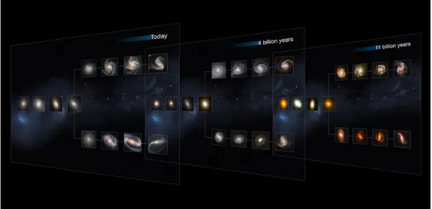
Figure 3.1: This image illustrates the Hubble sequence for galaxy classification at three different cosmological epochs. It shows the evolution of each galaxy type along cosmic time up to the present-day universe where galaxies are fully formed with various shapes. These images come from the Hubble Space Telescope Cosmic Assembly Near-infrared Deep Extragalactic Legacy Survey (CANDELS). Credit: NASA, ESA, and M. Kornmesser (ESO)
After the discovery of galaxies, astronomers began to observe them, trying first to classify these objects according to their structure and morphology. After years of science, this led to the well known Hubble sequence or “Hubble tuning fork” diagram which separates galaxies according to their morphology. First published by E. Hubble in 1926, it has been extended by de Vaucouleurs in 1959 and Sandage in 1961. Two main types of galaxies dominate this diagram: ellipticals and spirals. Figure 3.1 (left side, present-day diagram) shows the ellipticals on the left branch of the diagram and the spirals galaxies on the right. The spirals galaxies are further divided into spirals with (bottom branch) or without (top branch) bars in their central regions. The lenticular galaxies, S0, are placed at the center of the fork between the ellipticals and the spirals galaxies. These galaxies tend to
have a bright central bulge surrounded by disk-like structure but with no visible real spiral arm structures like in spiral galaxies.
The de Vaucouleurs classification system complements Hubble sequence with a more elaborated division of the spiral galaxies type, taking into account the presence of bars and rings. This was followed by many other works each trying to improve the sequence by enhancing for example the classification of spiral arms (eg. Elmegreen & Elmegreen 1982, 1987). Other classification systems exist like the Yerkes scheme developed by Morgan (1962), which is based on the shape and the central concentration of light in a galaxy image. However the morphological classification method introduced by E. Hubble is still the most commonly used.
This allowed scientists to classify galaxies in the nearby universe visually through structural features. However when we go further back in time these galaxies are still in their formation process. In Fig. 3.1 we can see that these galaxies, if we go back to 4 and 11 billion years ago, are smaller and more peculiars. It illustrates that galaxies have indeed evolved along cosmic time.
Another result brought by Hubble is the relation between the apparent velocity of galaxies (V ) and their distance (D), expressed by the following equation :
V = H × D (3.1)
This relation is called Hubble’s law (Hubble 1929), where H corresponds to the Hubble Constant. The last estimate of this constant was measured by Planck with
H = 67.8 km s−1 Mpc−1 (Aghanim et al. 2018). For the following parts of the
thesis, we introduce the notion of “redshift”, which happens when the light emitted by a moving object increases in wavelength and is thus shifted to the red part of the electromagnetic spectrum. The redshift, z, is linked to the observed wavelength of the source λobs and its vacuum wavelength λ0 by the equation:
λobs = λ0(1 + z) (3.2)
In astronomy, this shift in wavelength is linked to the distance of the object in the universe. Because of the expansion of the Universe, a galaxy that is farther
28 3.1. Galaxy evolution since the early universe
away will have a larger receding velocity, and thus a larger redshift. This means that if we look at galaxies at higher redshift we look further back in time. We can thus study galaxy evolution by observing the galaxies at different redshifts. Modern telescopes are now powerful enough to observe galaxies at redshift beyond 6, probing galaxy populations in the early universe.
3.1.2
Evolution of the star formation rate
Figure 3.2: The history of cosmic star formation derived from far-infrared and far ultra-violet rest-frame measurements on the right panel and on the whole range on the left panel. The different symbols correspond to the different survey data sets. Blue-gray hexagons: Wyder et al. (2005); blue triangles: Schiminovich et al. (2005); green pentagons and squares: Robotham & Driver (2011) and Cucciati et al. (2012); turquoise pentagons: Dahlen et al. (2007); dark green triangles: Reddy & Steidel (2009), magenta pentagons: Bouwens et al. (2012a,b); black crosses: Schenker et al. (2013); brown circles: Sanders et al. (2003); orange squares: Takeuchi et al. (2003); red open hexagons: Magnelli et al. (2011); red filled hexagons: Magnelli et al. (2013); dark red filled hexagons; Gruppioni et
al. (2013). Credit: Madau & Dickinson, 2014
Some fundamental galaxy properties are used by astronomers to trace their evolution. Such is the case for the star formation rate (SFR) which gives the mass of stars (in solar units) formed by a galaxy per year. To quantify the star formation rate, studies generally rely on the observed luminosities and luminosity functions (eg. Madau & Dickinson 2014).
Various methods and indicators are used to estimate the SFR. The typical star formation rate indicators are often the ultra-violet (UV) luminosity which gives a direct estimate of the young stellar population, Hα luminosity and nebular emission lines, or the infra-red (IR) luminosity. Assuming a linear scaling between the SFR and the continuum luminosity integrated over a fixed band, evolutionary synthesis models infer the relation between the SFR per unit mass and the luminosity.
From the evolutionary synthesis model of Kennicutt (1998a, 1998b) the SFRs inferred from the three luminosities are described as:
SF RU V(M yr−1) = KU V × LU V (erg s−1Hz−1) (3.3)
SF RHα(M yr−1) = KHα× LHα(erg s−1) (3.4)
SF RIR(M yr−1) = KIR× LIR(L ) (3.5)
The value of the conversion parameter K depends of the star formation history, the metal-enrichment history and the IMF chosen for the evolutionary synthesis model (Kennicutt 1998a, 1998b; Madau & Dickinson, 2014; Smit et al., 2012; Katsianis et al., 2017).
In their work, Madau & Dickinson (2014) take into account several data sets acquired from different surveys performed with instruments such as Spitzer or
GALEX. In the estimation of the galaxy luminosity the dust attenuation along the
line of sight must be taken into account. A corrective term must then be applied. From the computed integrated luminosity density, the cosmic star formation density is estimated using the appropriate equation 3.3, 3.4 or 3.5.
Figure 3.2 shows the results of this study. A clear picture is emerging, it seems that the cosmic star formation reaches a maximum around z ≈ 2.5 and then decreases for lower redshifts. The Universe was much more active in the past with a star formation rate higher than what is seen for z < 1. Katsianis et al. (2017) investigate the evolution of the cosmic star formation rate density for z = 0 − 7 from different cosmological hydrodynamic simulations and observations and found the same evolutionary trend as Madau et & Dickinson (2014). Despite differences in the measurements the different SFR indicators produce consistent results. They
30 3.1. Galaxy evolution since the early universe
suggest that the evolution of the cosmic star formation is mostly determined by a balance between gas accretion and feedback processes.
3.1.3
Evolution of the stellar mass density of galaxies
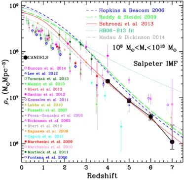
Figure 3.3: The integrated stellar mass density estimated from various studies over a large redshift range. Credit: Grazian et al. (2015)
Another powerful proxy to characterize galactic evolution is to investigate the stellar mass density of galaxies across cosmic time.
Several studies (Bundy et al., 2005; Mortlock et al., 2011; Madau & Dickinson, 2014; Duncan et al., 2014; Grazian et al., 2015; Davidzon et al., 2017) are in good agreements over the trend of the stellar mass density evolution. One of the methods usually used to derive the stellar mass density is to first estimate the stellar mass of large samples of galaxies, often by fitting the spectral energy distribution (SED) of galaxies. This method consists in using model predictions and minimization procedures to best fit the observed SED using a set of template spectra. The best fit obtained gives the information on the physical properties of the observed galaxy, like the redshift, stellar mass, star formation rate, dust mass, or metallicity. Then construct the stellar mass function for different redshifts by calculating the
number of galaxies per co-moving volume and mass range for each redshift interval. The last step is to integrate over the Schechter function (Schechter 1976) between two mass limits to derive the total stellar mass contained into galaxies for each redshift interval per co-moving volume.
Figure 3.3 shows the redshift evolution of the stellar mass density from several analyses (Grazian et al., 2015). It seems that the stellar mass density evolves greatly with redshift with a swift increase of the mass between 1 < z < 4. About half of all stellar mass is assembled in galaxies by z = 1.5. Many authors conclude that the majority of the stellar mass of a galaxy is already in place before the star formation seems to stop and suggest that star formation alone is not enough to explain these massive galaxies and other building processes must be at works, for example galaxy mergers.
3.2
Galaxy mergers versus cold gas accretion
As discussed above, strong evidence that galaxies have undergone a significant evolution over cosmic time were found over the past decades. However, what are the main driving mechanisms behind the growth of these galaxies remains a fundamental question. We now believe that galaxy mergers and cold gas accretion are the main processes contributing to the build-up of galaxies since the early universe.
3.2.1
The role of cold gas flows in feeding galaxies
Galaxies are not closed-box systems, they interact with their environment. In the cold gas accretion scenario, fresh cool gas falls onto the galaxy from cold gas streams following the cosmic web of large-scale structures (see Fig. 3.4).
Several observational studies and hydrodynamic simulations show that this process is needed by galactic evolution models as a way to supply star formation on long timescales, as well as to explain chemical evolution models (Chiappini et al. 2001; Semelin & Combes 2002; Bournaud et al. 2011; Anglés-Alcázar et al. 2017; Qu et al. 2017; Rodriguez-Gomez et al. 2016). This process is well studied trough
32 3.2. Galaxy mergers versus cold gas accretion
Figure 3.4: This is an artist’s view of a galaxy in the process of pulling in cool gas from its environments. The bright object to the left of the galaxy is a background quasar which shine through the accreted gas flows. It illustrates how we find indirect evidence of the cold gas accretion theory through ingenious methods such as, in this case, the use of the background quasar to probe absorption features due to the gas inflows and outflows. Credit: ESO/L. Calçada/ESA
numerical simulations (see Fig 3.5), where the accretion of gas along filaments comes from the growth of dark matter halos which pulls the cold baryons along.
While it is established that gas accretion plays an important role in galaxy growth, the details of how this mechanism takes place is still unknown. Indeed, direct observational evidence of this phenomenon have been difficult to obtain. Only indirect proofs have been available up to now, as for example the so-called “G-dwarf problem”. Indeed, the metallicity distribution of G-stars in the Milky Way does not seems to be consistent with predictions from chemical evolution models unless some fresh gas infall is added (Schmidt 1963; Pagel & Patchett 1975).
Another indirect argument for gas accretion comes from the presence of expected absorption features along background quasar sight-lines (see Fig. 3.4; Caimmi 2008; Sancisi et al. 2008; Bournaud et al. 2011; Stewart et al. 2011a; Bouché et al., 2013, 2016). Since the infalling gas is not rotationally supported (Stewart et al. 2011a),
Figure 3.5: From numerical simulations, this picture shows a disk galaxy accreting gas along cosmic web filaments at z ≈ 3. The shock heated gas around the galaxy is colored in red, in blue we can see the cold gas stream connecting to the edge of the disc and in green the metal rich gas stripped from smaller satellites galaxies around. In their related paper, the authors conclude that with its interactions with hot halo gas, the accreted cold gas seems to settles into large disc-like objects and thus explain that clump-cluster or chain-galaxies could come from enhanced gas accretion from cold dense filaments and interactions with smaller galaxy companions. Credit: Agertz et al, 2009.
if we observe the absorption along bright background sources, like quasars, its kinematics is expected to be offset from the galaxy own systemic velocity. Bouché et al. (2013) present an analysis of the absorbing gas properties such as kinematics, metallicity and dust properties for a star forming galaxy at z ≈ 2.3, using a background quasar at a distance of 26 kpc from the galaxy. In a more recent article (Bouché et al. 2016), a similar analysis was performed on a z = 0.91 low-mass star-forming galaxy with data from the new Multi Unit Spectroscopic Explorer (MUSE). Distinct signatures, extended up to 12 kpc, like the ones expected for a cold gas flow were found. The associated infalling gas accretion rate is estimated to be at least two times larger than the SFR.
Conselice et al. (2013) also argue that accretion from the intergalactic medium is necessary to sustain star formation in galaxies and could be the dominant mechanism for new stellar mass assembly for the most massive galaxies at 1.5 < z < 3, with 66% of all star formation at this epoch resulting from gas accretion. This result is corroborated by some cosmological simulations which estimate that the mean
34 3.2. Galaxy mergers versus cold gas accretion
fraction of mass assembled by accretion is about 77%, compared to 23% for galaxy mergers (L’Huillier et al., 2012).
Recently, from narrow-band imaging, a large and luminous filament, was discovered near the quasi-stellar object QSO UM287 at z ≈ 2.28. In their paper, Martin et al. (2015) proposed a spectroscopic investigation of the emitting structure. They find that the region may be a giant proto-galactic disk connected to a quiescent filament which extend behind the virial radius of the halo. Moreover its geometry supports a cold accretion flow approach (Martin et al., 2015).
3.2.2
The role of galaxy mergers in galaxy evolution
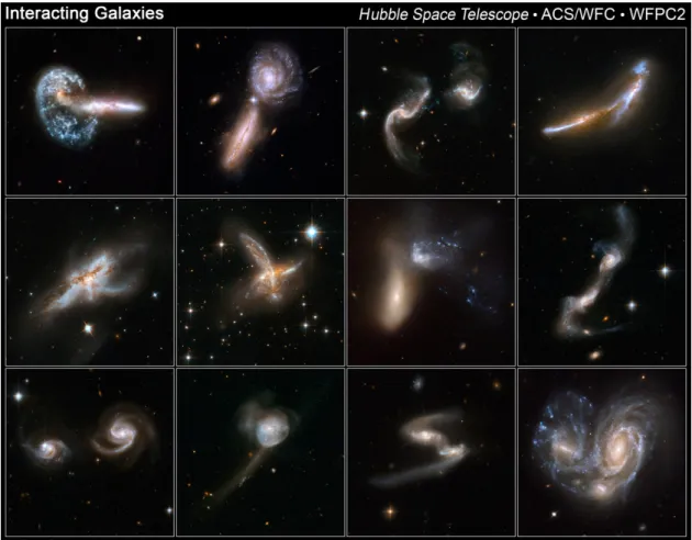
Figure 3.6: Hubble images of galaxies in the merging process. Credit: NASA/ESA,
Hubble collaboration and A. Evans.
Galaxy mergers are among the most spectacular events observed in the universe (Fig 3.6). Two galaxies colliding can lead to a galaxy merger if they do not have
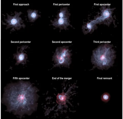
Figure 3.7: From hydrodynamical simulations, the time sequence of a galaxy merger event. The two galaxies have a mass ratio of 1:2. The initial separation between the galaxies is set near the sum of the two virial radii. Credit: IAP, M. Volonteri
enough momentum to resist the gravitational pull between them. This results in the two galaxies orbiting each other in a sort of dance before succumbing to one another and merging into a single galaxy. Various parameters such as relative velocity, angle of the collision, size, composition or mass of galaxies can affect the result of two colliding galaxies.
These events have been well studied in the nearby universe through both observational and simulation analyses. Figure 3.7 shows a simulation of two galaxies in the process of merging. As the time passes the two parent galaxies get closer until they interact for the first time, which is call the first pass or first pericenter passage. Then the two galaxies will start to move away from each other before being pulled again toward each other. Depending on many factors such as the mass ratio between the two galaxies, orbital configurations, gas fractions and others, the galaxies can
36 3.2. Galaxy mergers versus cold gas accretion
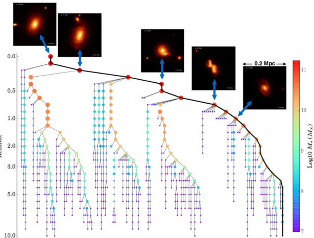
Figure 3.8: An example from Qu et al. (2017) of a galaxy merger history from numerical simulation. We follow a galaxy through the main branch (black line) that experience several merging and interactions events, for redshift between 0 < z < 1, additional images of the galaxy’s stellar mass distribution is displayed at the top. The size and color of the symbols are logarithmically scaled with stellar mass. Credit: Qu et al., 2017.
suffer several passes before merging. At each close pass, the galaxies can strip material from each other, creating tidal tails and other morphological disturbances. It can also trigger an enhancement of the star formation activiy within the galaxies and fuel starbursts (Joseph & Wright 1985; Di Matteo et al. 2007; Kaviraj 2014). This phenomenon is a relatively slow one, indeed the typical timescale for a merger between two massive galaxies of approximately the same mass is around 1 Gyr (Kitzbichler & White 2008; Jian et al. 2012; Moreno et al. 2013).
It is acknowledged that galaxy merger play a key role in the formation and evolution of galaxies. They are in part responsible for shaping galaxy morphologies, internal structures and dynamics (e.g. Mihos & Hernquist 1994; López-Sanjuan et al., 2012; Perret et al. 2014; Lagos et al. 2017). For example equal mass spiral
galaxy mergers are known to form elliptical galaxies. It is believed that even mergers with small companion galaxies can affect the disk of spiral galaxies and multiple mergers of different mass ratios can transform spiral galaxies into lenticular or elliptical systems (Bournaud et al., 2007).
Galaxy merger have also an important role in the mass assembly of galaxies (De Lucia & Blaizot 2007; Guo & White 2008). N-body/Hydrodynamical simulations are powerful tool to study the relative contributions of mergers to the stellar mass assembly of galaxies (Genel et al. 2009; Rodriguez-Gomez et al. 2016; Qu et al. 2017). The history of galaxies can be inferred from merger trees (see Fig 3.8). Thanks to these simulations, a given galaxy can be followed as it evolved through severals merging events along cosmic time. From Illustris simulations, Rodriguez-Gomez et al. (2016) estimated that about 50% of the ex-situ stellar mass of galaxies come from merger of equal mass galaxies and 20% from mergers with a small companion.
To conclude, understanding how galaxy mergers influence galactic evolution is a key aspect for every galaxy formation models.
Galaxy mergers classification
Different properties can be used to classify galaxy mergers. For example, using the gas richness of the galaxies allows the distinction between wet, dry and mixed merger (Lin et al. 2010). A merger between gas-rich or blue galaxies is called a wet merger. These interactions generally can trigger a larger amount of star formation, and even produce quasar activity. A dry merger involves two gas-poor or red galaxies, although they do not have a strong impact on the star formation they still contribute to the mass growth of the galaxies. Lin et al. (2010) suggest that dry mergers are important in the mass assembly of massive red galaxies in dense environments, like galaxy groups or clusters, contributing to 38% of their mass accretion in the last 8 billion year. Lastly, a mixed merger, as indicate by his name, is a merger between a gas-rich and gas-poor galaxy.
The most common way used by astronomers to distinguish between galaxy mergers is to use the mass ratio between the two galaxies as a proxy. Thus major
38 3.3. How can we detect galaxy mergers ?
mergers occur when two galaxies of approximately the same size or mass collide. This is a violent event which often trigger star formation and strongly impact the morphology of the galaxies. For example, major merger are well known for forming elliptical galaxies from spiral parent galaxies. In comparison, minor mergers involve a companion galaxy significantly smaller and less massive than the primary galaxy (the most massive of the two). The satellite galaxy will be completely stripped from its gas and stars by the other galaxy who will suffer little effect. It is some sort of cosmological cannibalism. These events are more frequent in the nearby universe than major mergers. As a simple example of minor merger, our own galaxy, the Milky Way, seems to currently absorb smaller satellite galaxies like the Canis Major dwarf galaxy, and possibly the Magellanic Clouds. Minor mergers also play a role in galactic evolution for example they contribute significantly to the size growth of quiescent galaxies (Newman et al., 2012; Bédorf et al., 2013) and to the cosmic star formation budget (Kaviraj, 2014).
The relative contribution of major and minor mergers to the build-up of galaxies is still unclear. Although major mergers play a key role at low redshift (López-Sanjuan et al., 2012), is it the same in the early universe ? Some recent studies imply that major mergers are not the primary drivers behind galaxy growth at high redshift (Williams et al., 2011; Kaviraj et al., 2014) and other mechanisms like minor merger or cold gas accretion are at play.
3.3
How can we detect galaxy mergers ?
Galaxy mergers and cold gas accretion are mechanisms that play a key role in galaxy evolution. However, the relative importance of both phenomena remains uncertain, since the total amount of mass accretion onto galaxies by merging is still poorly constrained, especially in the early epoch of galaxy evolution due to the difficulty to observe these events at high redshift.
Several methods have been used to investigate merging activity across cos-mic time, for instance by identifying mergers through perturbations in galaxy
morphologies or by close pair counts of galaxies. We detail these two methods in the following sub-sections.
3.3.1
Morphological studies
The study of the structure of galaxies is a very powerful method for determining galaxies that are in the process of merging. During these interactions, galaxy mergers deform the morphologies of the galaxies involved, some of them even become peculiar. This is particularly true for major mergers.
The main methods to detect galaxy mergers trough morphological clues use the CAS (concentration, C; asymmetry, A; clumpiness, S), Gini/M20 parameters or
visual identification (Le Févre et al. 2000; Conselice et al. 2003, 2008; Lotz et al. 2006; Kampczyk et al. 2007; Bluck et al. 2012; Casteels et al. 2014).
The CAS quantitative morphological system (Conselice et al., 2003, 2006; 2014) uses the concentration, asymmetry, and clumpiness of a galaxy’s light profile to distinguish galaxies in different phases of evolution in a three dimensional CAS space. Merging galaxies are identified mostly through the asymmetry index A, which accounts for the asymmetric appearance of a galaxy after a rotation of 180 degrees along the galaxy’s line of sight center axis. Galaxy mergers generally present an important asymmetry value higher than the clumpiness parameter. This selective condition translating as A > 0.35 and A > S allows the potential identification of about 50% of real mergers (Conselice, 2014). This method is more sensitive to major mergers (Conselice et al., 2003; Bluck et al. 2012).
Another approach uses the Gini or G and M20 indicators which is another
non-parametric measure of galaxy morphology. In Lotz et al. (2004; 2006) they are described as: the relative distribution of the galaxy pixel flux values, G, and the second-order moment of the brightest 20% of the flux of the galaxy. Galaxy mergers can thus be identified using the following relation between G and M20:
G > −0.115 × M20+ 0.84 (Lotz et al., 2006). This relationship is not sensitive to a
40 3.3. How can we detect galaxy mergers ?
All these morphological methods trace post-mergers or galaxy mergers when the interactions between galaxies have already begun, contrary to the study of the close pairs which favors the detection of possible future mergers, only identifying close pair of galaxies. These methods are applicable to low redshift. However, instruments spatial resolution is often too poor to be able to calculate these morphological parameters at high redshifts (z > 3). Moreover morphological disturbances are not always related to merger events, as suggested by galaxy kinematics (e.g. Förster Schreiber et al. 2009, 2011), this is even more the case for high redshift. Therefore most studies at high redshift z > 2 have favored the close pair counts method to probe merger abundance.
3.3.2
Close pair counts of galaxies
A more statistical approach to trace merger abundance is through galaxy close pair counts analysis. Before they merge all these systems appeared as gravitationally bound pairs of two galaxies. Thus the idea is to detect close pairs of galaxies as a proxy for potential future mergers since these close pairs are expected to merge within an estimated timescale.
Ideally, close pairs of galaxies would be identified based on their true physical separation distance (i.e. in real space), however it is not directly applicable to observational survey.
While the first analyses on galaxy close pairs used the apparent angular separation and angular diameter of the galaxies as selection criteria (Turner 1976a; Peterson 1979), in more recent works a close pair is defined as two galaxies within a limited projected angular separation, rp < rmaxp (kpc), and line-of-sight relative
velocity, ∆v < ∆vmax, based on the redshift of the two galaxies (Patton et al.
2000; de Ravel et al. 2009; Lopez-Sanjuan et al. 2013; Tasca et al. 2014; Man et al. 2016). The value range of the selection criteria used for the detection of close pairs of galaxies can vary according to the study.
Close pairs counts analysis have been conducted on both photometric and spectroscopic surveys. While photometric surveys have the advantages of providing
large samples of galaxies, which bring strong statistic for the estimation of the close pair fraction and rate, photometric redshifts are less reliable than spectroscopic ones, which usually translate in a velocity limit criterion higher than the one for spectroscopic survey. Thus the probability that the close galaxy pair will finally merge is lower, contaminating the sample by possible chance pairing (i.e. pairs which will satisfy the selection criteria but are not gravitationally bound). Using spectroscopic redshift is a more robust way to confirm the physical closeness of the two galaxies. For spectroscopic surveys a selection criterion of ∆v > 300 − 500 km s−1 is often used, which offers a good compromise between contamination
and pair statistics (Patton et al. 2000; Lin et al. 2008). The value range for the projected separation criterion varies a lot in the literature, 0 − 10 < rp <
25 − 50 − 100 − 200 h−1kpc. The difference in the selection criteria adopted can
make direct comparisons difficult.
During this thesis, I use the close pairs count method in my analysis to infer the merger fraction and rate evolution in the MUSE data sets.
3.4
The galaxy merger fraction and rate up to
z ≈ 3
The merger fraction is usually defined as the number of galaxies involved in a merger divided by the number of individual galaxies in the sample for a given redshift interval. Various corrective terms must be applied to take into account potential selection effects and completeness, since observations are limited in volume and luminosity. The galaxy merger rate, which is the number of mergers suffered by a galaxy per Gyr, can then be derived from the fraction using merger time scales.
Until this PhD thesis, the galaxy major merger fraction and rate was rather well constrained from morphological and close pairs counts analyses up to z ∼ 1. Overall, the major merger fraction is only about 2% in the nearby universe, then increases with redshift up to z ∼ 1 (Lin et al. 2008; Bundy et al. 2009; de Ravel et al. 2009; Lopez-Sanjuan et al. 2012). The evolution of the major merger fraction can be parametrized as a function of redshift as a power law of the form (1 + z)m with
42 3.4. The galaxy merger fraction and rate up to z ≈3
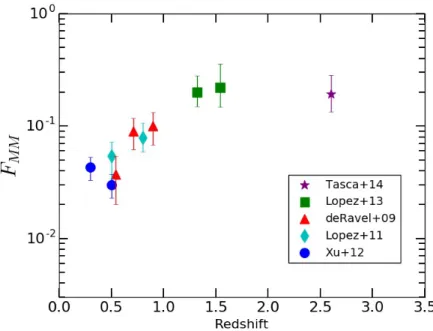
Figure 3.9: Evolution of the major merger fraction from spectroscopic close pair counts studies. Each symbol refers to a different survey: Tasca et al. (2014; purple star), Lopez-Sanjuan et al. (2011, cyan diamonds; 2013; green squares), de Ravel et al. (2009; red triangles), and Xu et al. (2012; blue points).
several values for the coefficient m reported in the literature, ranging from 0 to 5 (e.g. Le Fèvre et al. 2000; Kampczyk et al. 2007; Kartaltepe et al. 2007; de Ravel et al. 2009; Lotz et al. 2011, Keenan et al. 2014). This discrepancy between measurements usually comes from the various methods and selection criteria adopted.
Beyond z ∼ 1.5, photometric and spectroscopic close pairs count studies report that the major merger fraction/rate seems either to increase up to z ∼ 2 − 3 (Bluck et al. 2009; Man et al. 2012, 2016) for flux-ratio selected samples, or reach a maximum at z ≈ 2 and then remains constant or turn down at higher redshift for mass-ratio selected samples (Lopez-Sanjuan et al. 2013; Tasca et al. 2014).
The large scatter between these results can be attributed to the selection criteria used for identifying major mergers either through the stellar mass ratio of the two galaxies, or their luminosity ratio. Indeed Man et al. (2016) reveal that by using a flux-selected ratio as proxy for major merger, the sample is in fact contaminated by a large number of minor mergers, with a mass ratio lower than 1:4. Thus flux-ratio-based galaxy merger fractions and rates must be treated carefully.
Figure 3.10: Comparison of the major merger rate derived from CANDELS and SDSS surveys for mass-ratio (filled red points) and flux-ratio (open red points) selected samples and for massive galaxies (M? > 2 × 10¹⁰ M ). The major merger rate from Mantha et
al. (2018) photometric close pair counts analysis is also compared to previous works such as Lotz et al. (2011; dashed and solid magenta line), Man et al. (2016; blue line and associated uncertainties), as well as simulation predictions from Rodriguez-Gomez et al. (2015; black line) and Hopkins et al. (2010; green line). Lastly, the analytical predictions of major merger rate for Mhalo ≈ 1012 M dark matter haloes R ≈ (1 + z)2.5
is represented by the brown dashed line (Neistein & Dekel, 2008; Dekel et al., 2013). Credit: Mantha et al., 2018
Figure 3.10 illustrates the different evolutionary trends of the major merger rate obtained with either mass ratios or flux ratios (Mantha et al. 2018). Figure 3.9 shows the evolutionary trend of the major merger fraction along cosmic time obtained from a compilation of different spectroscopic close pairs counts studies with a mass-ratio selection criteria. As discussed previously, the major merger fraction seems to converge toward a value around 20% at z = 2 − 3 (Lopez-Sanjuan et al., 2013; Tasca et al., 2014). This evolutionary trend seems to be in agreement with recent predictions of cosmological simulations, like Horizon-AGN (Kaviraj et al. 2015) or EAGLE (Qu et al. 2017).
At the beginning of my PhD thesis, no measurement beyond z ∼ 3 were reported due mainly to the difficulty of detecting spectroscopic close pairs of
44 3.5. Organization of the thesis
galaxies at these redshifts.
As for the evolution of the minor merger fraction and rate of galaxies, these quantities were almost unconstrained, with very few attempts so far (eg. Lopez-Sanjuan et al. 2011, 2012, Lotz et al., 2011, Bluck et al., 2012).
In this context, the exquisite new data provided by second generation instruments such as the Multi Unit Spectroscopic Explorer (MUSE) are ideal to study pair counts and derive merger fractions and rates at high redshift.
3.5
Organization of the thesis
In this manuscript, I present my work on the investigation of cosmological evolution of the galaxy merger fraction and rate from MUSE deep fields. The following chapter describes the MUSE instrument and project as well as the data sets used in this study. I detail MUSE deep observations over four different regions of the universe, the Hubble Deep Field South and the Hubble Ultra Deep Field, the galaxy cluster Abell 2744 and a small region in the COSMOS field centered around the galaxy group GR30. The methods used to derived redshift measurements and other properties are also summarized in this section.
In chapter 5, I present my first analysis of the major merger fraction evolution from the first two deep MUSE fields, the Hubble Ultra Deep Field and the Hubble Deep Field South, which has been published in the Astronomy & Astrophysics journal (Ventou et al. 2017). I explain the method used to highlight the presence of companion galaxies orbiting around another and give estimates of the major merger fraction up to z ≈ 6 for different stellar mass ranges of galaxies. Results are compared to previous close pair count studies and recent simulation predictions. The second part of my thesis focused on the improvement of the galaxy close pairs criteria using Illustris cosmological simulations to investigate the relation between close pair selection criteria (separation distance and relative velocity) and whether the two galaxies will finally merge. I extend my close pair study to the whole data set (four deep MUSE fields in total) and derived robust estimates of the major and
minor merger fractions along cosmic time. This work is presented in chapter 6 in a paper format that will be submitted soon to the Astronomy & Astrophysics journal.
Finally, in the last chapter, I convert my results of the merger fraction in major and minor merger rates. In this section, I also discuss the uncertainties of the merger time scale and its influence on the merger rate.
4
MUSE observations
Contents
4.1 The project . . . . 47 4.2 The instrument . . . . 49 4.3 MUSE deep fields . . . . 52 4.3.1 Hubble Deep Field South . . . 52 4.3.2 Hubble Ultra Deep Field . . . 55 4.3.3 Abell 2744 . . . 60 4.3.4 COSMOS-Gr30 . . . 63
4.1
The project
The Multi Unit Spectroscopic Explorer, known as MUSE, is the culmination of a decade of research and development. Commissioned in 2014, Muse is installed on the Nasmyth focus of Yepun, the fourth Very Large Telescope at the Paranal Observatory in the middle of the Chilean Atacama desert. The project was born as an answer to the European Southern Observatory (ESO) call for proposals for second generation VLT instruments in early 2000s. The MUSE instrument is based on an innovative concept: coupling the capabilities of an imager and spectrograph in one device. The outcome is a unique and powerful instrument able to cover a large field of view with high resolution and acquire spectra for each pixel at the same time.
48 4.1. The project
Figure 4.1: Photographs of MUSE on the Nasmyth focus of Yepun (UT4), one of the Very Large Telescope at the Cerro Paranal Observatory in Chile. This was taken in September 2016 during my stay at the VLT Observatory for a GTO run on behalf of the MUSE consortium (left image). The right image shows the recent coupling of the MUSE instrument with the Adaptive Optics Facility called "GALACSI". The four Laser Guide Stars Facility point to the sky creating artificial stars used to determine the atmospheric conditions.
Credit: Emmy Ventou, Roland Bacon.
The project is supported by seven European research institutes: • The Centre de Recherche Astrophysique (CRAL) at Lyon, France • The Potsdam Astrophysikalisches Institut (AIP), Germany
• The Institut de Recherche en Astrophysique et Planétologie (IRAP) at Toulouse, France
• The Leiden Observatory, Netherlands
• The Göttingen Astrophysics Institute (AIG), Germany
• The Astrophysics department of the Zurich Polytechnic Institute of Technology (ETH), Switzerland
After being assembled and tested at CRAL in Lyon, the instrument finally arrived at Paranal 10 years after the beginning of the project where it successfully saw its first light on January 31, 2014. Promising exquisite data sets and new discoveries for modern astrophysics in the years to come. The MUSE consortium, lead by Roland Bacon (CRAL) the project PI, gather more than 80 researchers, including post-docs and PhD students. All interested in various science goals such as formation and evolution of galaxies, stellar population in nearby galaxies, quasars, super massive black holes, early stage of stellar evolution and small bodies in the Solar system. Members of the consortium get together for one week every six month during the famous “MUSE Busy Week”, where everyone present and discuss their science projects and work together to exploit MUSE wealth of data. Overall, the collab-oration obtained 255 observation nights as Guaranteed Time Observation. This observation time is shared between 14 science programs with ambitious goals such as: the MUSE deep investigation of the Hubble Ultra Deep Field ("MUSE-Deep" program, PI: Roland Bacon, CRAL), probing highly magnified regions of massive lensing clusters (PI: Johan Richard, CRAL), or studying how the environment affect galaxy evolution over the past 8 Gyr (PI: Thierry Contini, IRAP). During my thesis, I personally contributed to this last project.
4.2
The instrument
MUSE is a second generation integral field spectrograph, an innovative and powerful instrument merging imaging and spectroscopy capabilities in order to probe the universe in 3 dimensions (Fig 4.3). Compared to other Multi-IFU (Integral-Field Unit), MUSE does not require to pre-select the sources beforehand, leading to the potential discovery of objects not detected in the pre-imaging observations.
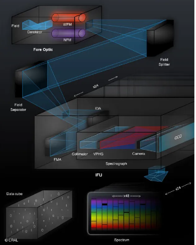
This is made possible by an assembly of 24 integral field spectrographs with a complex optical schematic system (see Fig 4.2). The light coming from the observed region in the southern sky enters the instrument and first encounters the derotator which compensate for the earth rotation. After being magnified by mirrors, the field-of-view is then splitted a first time into 24 optical beams by the field splitter
50 4.2. The instrument
Figure 4.2: Illustration of MUSE optical schematic system and data acquisition as described in section 4.2. Credit: CRAL
Figure 4.3: Illustration of a MUSE data cube, showing the three-dimensional view of the Pillars of Creation nebula in the Messier 16 region. The slices correspond to different views of the nebula at different wavelengths revealing motion and chemical gas components. Credit: ESO
and field separators. Each of these beams are distributed to the 24 spectrographs. The light is splitted again in 48 slices by a slicer, a revolutionary piece of technology composed of two set of 48 spherical mirrors (corresponding to the Image Dissector Array, IDA, and Focusing Mirrors Array, FMA, see Fig 4.2). Each slices follow their courses and enter the spectrograph where the light is dispersed according to its wavelength and finally arrive on a CCD detector of 16.8 million pixels.
The result is a 360 million pixels image containing 90 000 spectra covering a 4750 − 9300Å wavelength range (Fig 4.3). Overall, MUSE covers a 1 × 1 arcmin2
field-of-view in Wide Field Mode with a relatively good spectral resolution of
R = 2000 in the blue to 4000 in the red, for each 0.2” × 0.2” spatial pixels. MUSE
has also a second mode of observation, the Narrow Field Mode, which achieves a much better spatial resolution of 0.03” − 0.05” with a 0.025” spactial sampling, but covering a much smaller area 7.5” × 7.5”.
For this thesis only observations made with the Wide Field Mode were used, the corresponding MUSE fields are introduced in the next section.
52 4.3. MUSE deep fields
In June 2017, another adventure started with the coupling of the Adaptive Optics Facility (AOF) called "GALACSI" with the instrument, thereby improving the quality of the produced data set by correcting in real time the atmospheric distortion thanks to deformable mirrors. The Four Laser Guide Star Facility (4LGSF) consist in four laser beams pointed to the sky to mimic stars (see Fig 4.1, right image). These artificial guide stars are then used to compute atmospheric conditions and estimate the corrections to be applied to the deformable secondary mirror of the telescope. This ingenious system can thus compensate for the atmospheric disturbances up to one km above the telescope, where most of the atmospheric turbulences occurs. The resulting images are sharper, boosting further the capacity of the instrument to detect faint galaxies.
4.3
MUSE deep fields
Throughout these 3 years, my work was based on MUSE observations over 4 well known regions of the universe, the Hubble Deep Field South (4.3.1), the Hubble Ultra Deep Field (4.3.2), the Abell 2744 lensing cluster (4.3.3), and a galaxy group in the COSMOS field (4.3.4), obtained during a commissioning run in August 2014 (for the Hubble Deep Field South) and two years of the MUSE Guaranteed Time
Observations (GTO), from September 2014 to February 2016 (for the others).
4.3.1
Hubble Deep Field South
The Hubble Deep Field South (HDF-S) is part of Hubble legacy. After the success of the Hubble Deep Field North in 1995, it was decided to acquire another deep optical image of the distant universe but this time in the southern hemisphere. Thereby 3 years later, the first HST images of this part of the sky were assembled over 10 days between September and October 1998 (Williams et al., 2000), leading to fruitful studies and breakthrough scientific results in modern astronomy especially in the domain of the formation and evolution of galaxies over cosmic time. Since then many other ground- or space-based instruments have observed this region providing large amount of data that are complementary to each other. Hence it
Figure 4.4: View of the HDF-S in the WFPC2 F814W image. Different symbols and colors served to classify objects as: stars (blue), AGN (orange), nearby objects with z < 0.3 (cyan), objects identified solely with absorption lines (yellow), [O ii] λ3726,3729 (green) and C iii] λ1907,1909 (magenta) emitters, and lastly Lyα emitters with or without HST counterpart (red circles and red triangles respectfully) Image from Bacon et al. (2015).
was an appropriate target for the last commissioning run of MUSE, in order to test and optimize the performance of the instrument and data reduction pipeline in the first deep field targeted with MUSE.
In August 2014, a 1 × 1 arcmin2 area in the HDF-S centered around α =
22h32055.64” and δ = −60o33047”, chosen to include a bright-enough star for PSF
monitoring, was observed during 6 nights, resulting in a single field of 27 hours of total exposure time. The data cube reaches a 1σ emission line surface brightness limit of 1 × 10⁻¹⁹ erg s−1 cm2 arcsec−2, with a spectral resolution of ∼ 2.3 Å and a
54 4.3. MUSE deep fields
Figure 4.5: One of the Lyα emitters (MUSE ID 553) identified by MUSE without any HST counterpart at z ≈ 5.08. Top: HST images in 2 filters (F606W and F814W) as well as MUSE reconstructed white light and Lyα narrow band images centered around the emission line location delimited by a white circle. Bottom: The full spectrum smoothed with a 4 Å boxcar (in blue) and its 3σ error (in grey), followed by a zoom of the unsmoothed spectrum centered around the Lyα emission line. Image from Bacon et al. (2015).
spatial resolution ranging between 0.6” for the red end of the spectral range and 0.7” in the blue. 1D and 2D spectra were extracted for all continuum detected objects in the master catalog of Casertano et al. (2000) within MUSE field of view. A complementary approach allowed the identification of emission line sources through visual inspection or automatic detection tools. One of the strategy uses SExtractor (Bertin & Arnouts 1996) on a set of numerous narrow-band images created over the full wavelength range of the cube to enhance the detection of emission lines. Another strategy uses the LSDCat software (Herenz et al., 2016, 2017) to probe the cube for line emitters not associated with any continuum sources (see Bacon et al., 2015 for more details on data reduction and spectral extractions). Each spectra were inspected manually to identify emission or absorption features. A confidence level was assigned to the redshift measurement, 0 for undetermined redshift, 1 for redshift likely correct based on one feature, 2 secure redshift based on one feature and 3 for secure redshift based on several features. Overall the spectroscopic redshift of 189 sources were accurately measured up to a magnitude of
broad range 0 < z < 7. Location of these objects and their classification in different categories (stars, AGN, early-type galaxies, [O ii] λ3726,3729, C iii] λ1907,1909 and Lyα emitters, ...) is shown in Fig. 4.4. The biggest surprise was the discovery of 26 Lyα emitting galaxies not detected in previous HST deep broad-band images. An example of such object with no HST counterpart is given in Fig. 4.5. More details on data reduction and redshift determination as well as the source catalog can be found in Bacon et al. (2015).
This first data set offers a spectroscopic sample of galaxies spread over a large redshift range and extending to objects with very low luminosities. I started my thesis trying to identify close pairs of galaxies by probing the environment of the galaxies in this field and highlighting the possible presence of a companion galaxy. This leaded to the first discovery of close pairs of galaxy at very high redshift (z > 3) with robust spectroscopic measurements. Once my method was tested and optimized, I extended my analysis to other fields, starting with data obtained with MUSE over another Hubble Deep Field, the Hubble Ultra Deep Field.
4.3.2
Hubble Ultra Deep Field
Observed for the first time in 2003, the Hubble Ultra Deep Field known as HUDF is still up to this day the deepest image ever taken of the visible universe. Located in the Fornax constellation, the field cover a total area of about 11 arcmin2 with
a total exposure time around 270 hours taken over the course of 400 HST orbits around Earth. The first images published in 2004, reveal a zoo of ∼10 000 galaxies of various sizes, shapes, colors and redshifts. Some of them may be among the most distant astronomical objects known, dating back to 800 million years after the Big Bang, allowing scientists to delve deeper into their research on the formation and evolution of galaxies since early epoch of the universe (Beckwith et al., 2006).
Since then the HUDF was observed many times by all kind of instruments, notably in 2009 with the installation on the HST of a new camera, the Wide Field Camera 3 (WFC3/IR), capable of making exquisite infrared observations with an improved resolution over a wilder field of view. Relaunching the hunt for the most


![Figure 4.4: View of the HDF-S in the WFPC2 F814W image. Different symbols and colors served to classify objects as: stars (blue), AGN (orange), nearby objects with z < 0.3 (cyan), objects identified solely with absorption lines (yellow), [O ii] λ3726,37](https://thumb-eu.123doks.com/thumbv2/123doknet/2140774.8857/53.892.178.778.159.692/figure-different-symbols-classify-objects-objects-identified-absorption.webp)
