Numerical study of flow stream in a mini VAWT with relative rotating blades

Science Arts & Métiers (SAM)

is an open access repository that collects the work of Arts et Métiers Institute of Technology researchers and makes it freely available over the web where possible.

This is an author-deposited version published in: https://sam.ensam.eu

Handle ID: .http://hdl.handle.net/10985/6727

To cite this version :

Annie-Claude BAYEUL-LAINE, Sophie SIMONET, Aurore DOCKTER, Gérard BOIS - Numerical study of flow stream in a mini VAWT with relative rotating blades - In: 22nd International

Symposium on Transport Phenomena, Netherlands, 2011-11 - ISTP 22 - 2011

Any correspondence concerning this service should be sent to the repository Administrator : archiveouverte@ensam.eu

NUMERICAL STUDY OF FLOW STREAM IN A MINI VAWT WITH RELATIVE ROTATING BLADES

Bayeul-Lainé Annie-Claude, Simonet Sophie, Dockter Aurore, Bois Gérard LML, UMR CNRS 8107, Arts et Metiers PARISTECH

8, Boulevard Louis XIV 59000 Lille, France

annie-claude.bayeul-laine@ensam.eu, Sophie.simonet@ensam.eu, aurore.dockter-9@etudiants.ensam.eu,gerard.bois@ensam.eu

Abstract

Today, wind energy is mainly used to generate electricity and more and more with a renewable energy source character. Power production from wind turbines is affected by several conditions like w ind speed, turbine speed, turbine design, turbulence and changes of wind direction. These conditions are not always optimal and have negative effects on most turbines. The present turbine is supposed to be less affected by these conditions because the blad es combine a rotating movement around each own axis and around the main turbine’s one. Due to this combination of movements, flow around this turbine can be more optimized than classical Darrieus turbines. The turbine has a rotor with three straight blades of symmetrical aerofoil. Paper presents unsteady simulations that have been performed for one wind velocity and different blades stagger angles. The influence of two different blades geometry is studied for four different constant rotational speeds.

Keywords: Numerical simulation, performance coefficient, unsteady simulation, VAWT, vertical axis, wind energy, pitch controlled blades.

INTRODUCTION

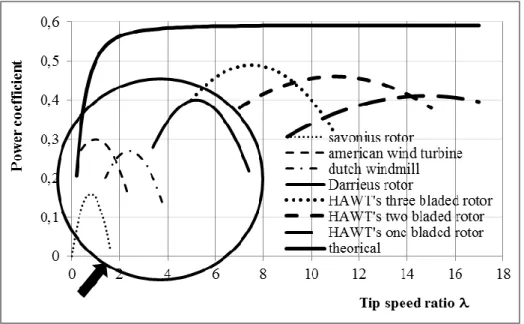
All wind turbines can be classified in two great families (Leconte P., Rapin M., Szechenyi E. (2001), Martin J. (1987)…): horizontal-axis wind turbine (HAWTs) and vertical-axis wind turbine (VAWTs). Figure 1 shows typical power coefficient of several main types of wind turbine: VAWTs work at low speed ratios.

A lot of works was published on VAWTs like Savonius or Darrieus rotors (Hau E.(2000), Paraschiviou I. (2002), Pawsey N. C. K. (2002)…) but few works were published on VAWTs with relative rotating blades (Bayeul-Lainé A.C. and al (2010), Cooper P. (2005, 2010), Dieudonné P. A. M.(2006)). Some inventors discovered this kind of turbine in the same time on different places (Cooper P., Dieudonné P.A. M. for example) and made studies these last ten years on this kind of VAWTs.

In 2008, F. Penet, P. de Bodinat and J. Valette gained an innovation price for an idea in which this kind of turbine is used to make a publicity panel lighted by wind energy. They created the society Windisplay to design, create and send such a product. The present study concerns this kind of VAWT technology in which each blade combines a rotating movement around its own axis and a rotating movement around turbine’s axis. It is an extensive study of a work given by this young people. This paper concerns the industrial one.

The aim of previous studies presented in 2010 (A.C. Bayeul-Lainé and al) was to give some results like contours of pressure, velocity fields and power coefficients, compared to relative steady blades. The benefit of rotating elliptic blades was shown: the performance of this kind of

turbine was very good and better than those of classical VAWTs for some specific initial blade stagger angles between 0 and 15 degrees. It was shown that each blade’s behaviour has less influence on flow stream around next blade and on power performance. The maximum mean numerical coefficient was about 32%.

Results were also compared to some numerical results.

The blade sketch needs to have two symmetrical planes because the leading edge becomes the trailing edge when each blade rotates once time around the turbine’s axis.

In the present study, new simulations were performed with straight blades. Results are compared between elliptic blades and straight blades: local results like contours of pressure, velocity fields, unsteady power coefficient, mean power coefficient.

Figure 1: Aerodynamics efficiencies of common types of wind turbines from Hau (2000). NON DIMENSIONAL COEFFICIENTS

The common non dimensional coefficients used for all wind turbines are: - Efficiency of a rotor, named power coefficient Cp

2 3 0 V S P C_p eff   (1)

In which Peff is the power captured by the turbine and

2 3 0 V S 

is the total kinetic energy passing through the swept area (Figure 3).

- Speed ratio l 0 V R_t   (2)

Where  is the angular velocity of the turbine, Rt is generally the radius blade tip (radius of

center of blade in case of this paper) and V0 the wind velocity.

- Reynolds number Re (Marchaj C. A.) based on blade’s length  L V Re 0  (3)

GEOMETRY AND TEST CASES

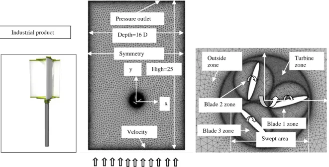
The sketch of the industrial product is shown in Figure 2. Blades have elliptic or straight sketches, relatively height, so a 2D model was chosen. The calculation domain around turbine is large enough to avoid perturbations as showing in Figure 3. Elliptic forms have minor radius of 75 mm and major radius of 525mm. Straight forms have a length of 1050 mm. Distance between turbine axis and blade axis is 620 mm.

Figure 2: Industrial product, mesh and boundaries’ conditions of VAWT with elliptic blades.

Figure 3: Zoom of the mesh of VAWT with straight blades for initial blade stagger angles of 0, 8 and 15 degrees.

Boundary conditions are velocity inlet to simulate a wind velocity in the lower line of the model (Re=560 000), symmetry planes for right and left lines of the domain and pressure outlet for the upper line of the domain. The model contains five zones: outside zone of turbine, three blades zones and zone between outside zone and blades zones named turbine zone. Turbine zone has a diameter named D (equal to the sum of R, plus the major radius of

Velocity inlet Symmetry planes Depth=16 D Pressure outlet High=25 D x y Industrial product Blade 2 zone Outside zone Blade 3 zone Turbine zone Blade 1 zone Swept area Azimuth angle 

blade plus a little gap allowing grid mesh to slide between each zone). Except outside zone, all other zones have relatively movements. Four interfaces between zones were created: an interface zone between outside and turbine zone and an interface between each blade and turbine zone. Details of zones are given in Figure 2.

Previous calculations, realized last year, for blade stagger angle comprised between -30 and 30 degrees, showed that flow is highly unsteady for initial blade stagger angles of -30 and 30 degrees. So, new calculations were performed for three initial blade stagger angles of 0, 8 and 15 degrees as it can be seen in Figure 3.

Mesh was refined near interfaces. Prism layer thickness was used around blades. The resulting computational grid is an unstructured triangular grid of about 60 000 cells, shown in Figures 3 and 4.

A time step corresponding to a rotation of 6.28e-3 radians was chosen to avoid to deform more quickly mesh near interfaces and to avoid negative cells. So a new mesh was calculated at each time step.

All simulations were realized with Star CCM+ V5.02 code using à k- model.

In a first part, global results like instantaneous and mean power coefficients and torques are compared between the two kinds of blades, for different speed ratios : 0.2, 0.4, 0.6 and 0.8 and for different blade stagger angles : 0, 8 and 15 degrees.

In a second part, fields for some special blade stagger angles and some special speed ratios are studied.

TORQUES AND POWER COEFFICIENTS

For this kind of turbine each blade needs energy to rotate around its own axis so real power captured by the turbine has to be corrected.

Code gives torque Mt around turbine axis for each blade, pressure forces and viscosity forces. So





Where O is the turbine centre, Gi the axis centre of blade i and df 

is elementary force on the blade i due to pressure and viscosity, so

i i ti C C M  ₁  ₂ (5) With





Real power was given by





Where 1, is the angular velocity of turbine and 2 is the relative angular velocity of each

2 1 2    (9)







And power coefficient by equation (1) in which swept area is those showed in Figure 4 for the cases with three rotating blades. Mean power coefficient is realized during the last revolution. RESULTS

Global results: power coefficients and torques

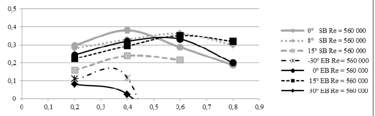
Figure 5 gives mean power coefficients for all test cases, for elliptic (EB) and straight blades (SB). This figure leads to next remarks:

- Better influence of straight blades comparatively to elliptic blades for an initial blade stagger angle of 0 degree (grey and black curves can be compared) for low blade speed ratios  (<0.4). Maximum mean power coefficient is better for straight blades but it decreases quickly when blade speed ratio decreases or increases from the value 0.4

- Bad influence of straight blades comparatively to elliptic blades for an initial blade stagger angle of 15 degrees

- Better stability of results for elliptic profile: Maximum Cp still remains for a large

scale of .

Figure 4: Mean power coefficient for different initial blade stagger angle with blade speed ratios

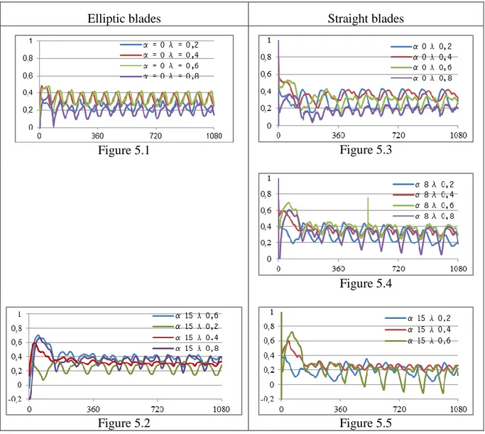
In order to explain previous remarks, it seems interesting to examine, among a lot of results, instantaneous global results for initial blade stagger angle a of 0 degree for blade speed ratio of 0.4 and 0.6 and also for  equal 15 degrees for  equal 0.2 and 0.4. Figures 5 give instantaneous power coefficients and figures 6 give torques for these values.

Comparison between Figure 5.1 and 5.3 shows, for  = 0.2, that mean values of power coefficient Cp is greater for straight blades but the range of changes is also greater. This leads

to more instability. For  = 0.4, Cp is also greater but more stable for straight blades. On the

contrary for  = 0.6 Cp is more stable for elliptic blades.

Figure 5.3 gives Cp for  = 8 degrees, more instabilities for  = 0.8 can be observed. These

instabilities are magnified in Figure 5.5 for =0.6. Calculations for  = 0.8 can’t be performed because of these instabilities. These results show the importance of relative velocities between wind velocity and angular velocity of turbine.

For = 15 degrees, comparison between Figure 5.2 and 5.5, for all values of , shows lower power coefficients for straight blades and higher instabilities. Moreover, these instabilities increased for =0.2 and  = 0.6. This can be explained by the fact that straight blades are less aerodynamic.

Elliptic blades Straight blades

Figure 5.1 Figure 5.3

Figure 5.4

Figure 5.2 Figure 5.5

Figures 5: Instantaneous performance coefficients with azimuth angle of blade 1

The global examination of all figures 5 leads to some remarks:

- For an initial blade stagger angle of 0 degree, straight blades give better results in value and in stability than elliptic blades for a blade speed ratio lower than 0.4. But for a blade speed ratio greater than 0.4, these conclusions are inverted.

- Results for elliptic blades are more stable: range of changes of mean power coefficient with blade speed ratios is lower, so this allows a greater range of blade speed ratio for elliptic blades. For straight blades, mean power coefficient decreases quickly.

- Comparison between these results show that straight blades is more influenced by low and high blade tip ratio than elliptic blades

- Maximum mean power coefficient for this kind of turbine is very interesting but the use of this kind of turbine needs some care in the aim of avoiding a fast decrease of performances.

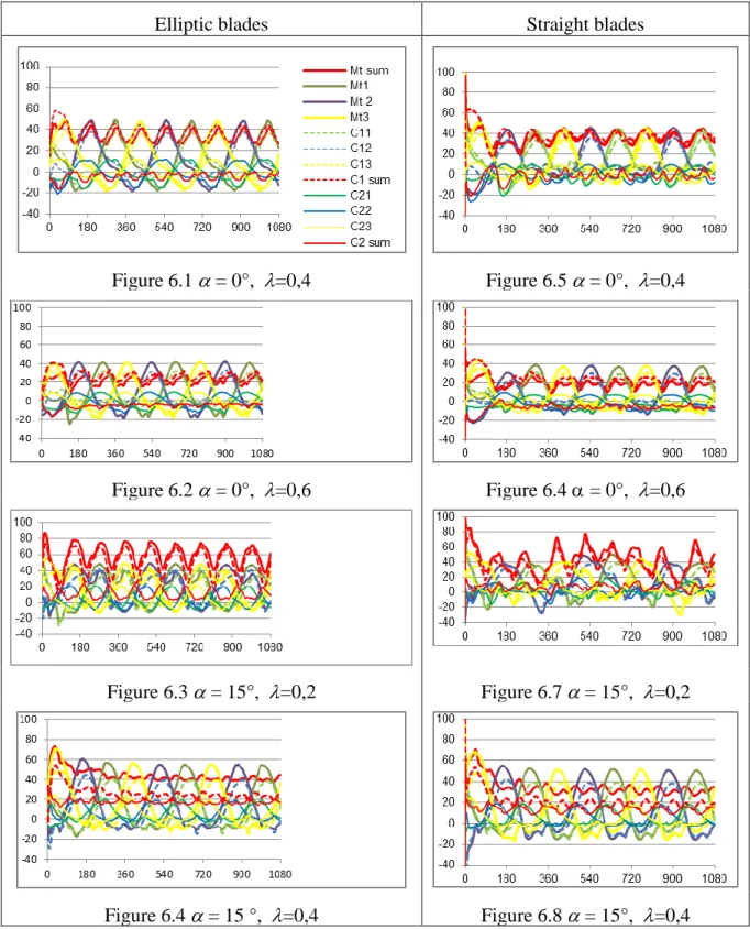
Figures 6 present evolution of torques with azimuth angle  of blade 1 for the values of

and previously chosen. Figures 6.1, 6.2, 6.4 and 6.5 (for = 0 degrees and <= 0.4) shows quite stable results and quite similar. This remark is besides confirmed by the examination of mean power coefficient (Figure 4).

Instabilities for  = 15 degrees and = 0.2 are also confirmed (Figure 6.7) when results are quite stable for  = 0.4 for the two kinds of blades (Figure 6.4 and Figure 6.8).

Elliptic blades Straight blades

Figure 6.1 = 0°, =0,4 Figure 6.5  = 0°, =0,4

Figure 6.2  = 0°, =0,6 Figure 6.4  = 0°, =0,6

Figure 6.3  = 15°, =0,2 Figure 6.7  = 15°, =0,2

Figure 6.4  = 15 °, =0,4 Figure 6.8  = 15°, =0,4

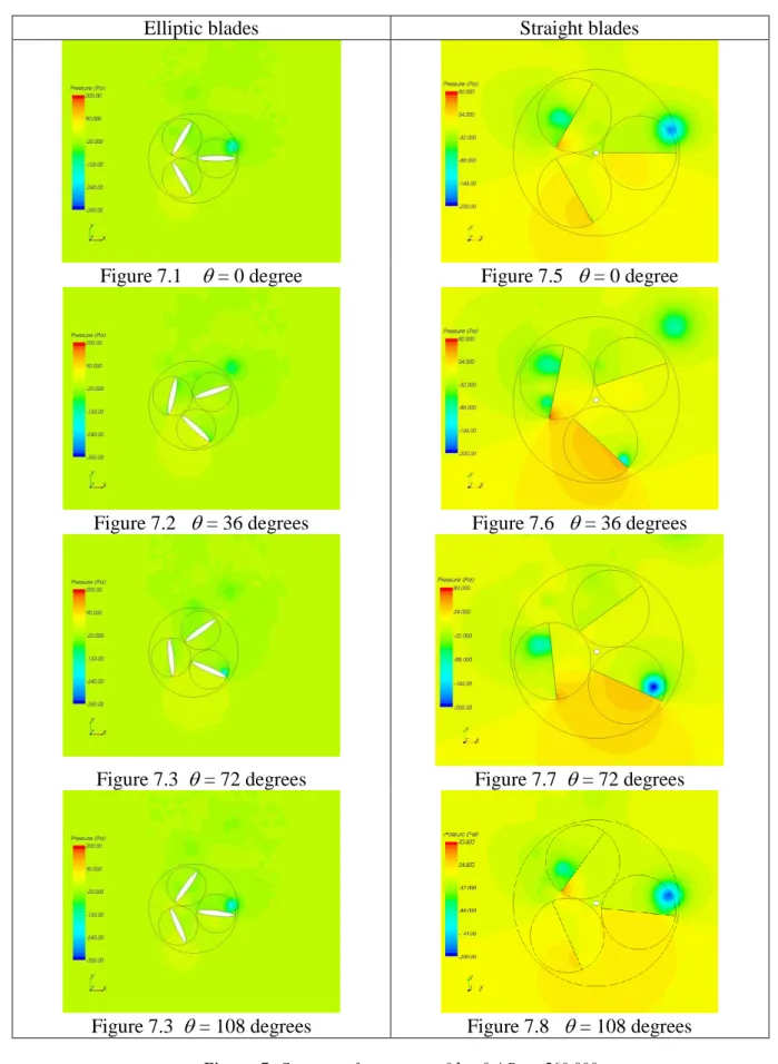
Local results: contours of pressure and vectors fields

Elliptic blades Straight blades

Figure 7.1 = 0 degree Figure 7.5 = 0 degree

Figure 7.2 = 36 degrees Figure 7.6 = 36 degrees

Figure 7.3 = 72 degrees Figure 7.7 = 72 degrees

Figure 7.3 = 108 degrees Figure 7.8 = 108 degrees

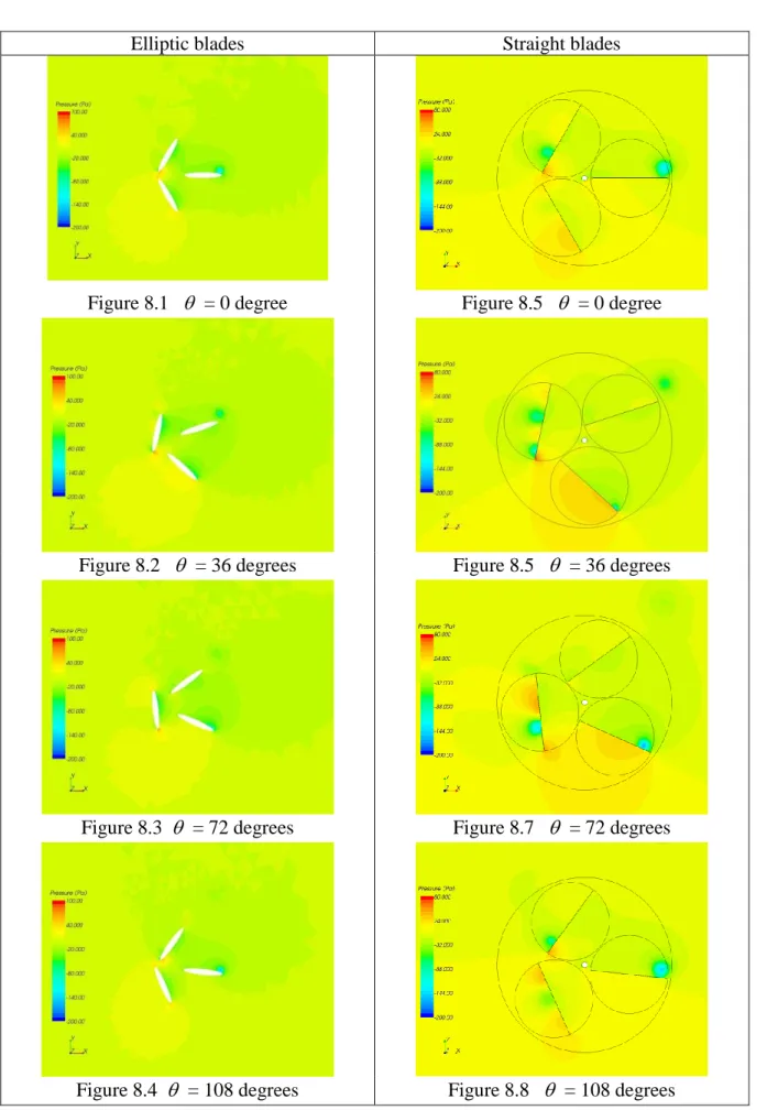
Elliptic blades Straight blades

Figure 8.1 = 0 degree Figure 8.5  = 0 degree

Figure 8.2 = 36 degrees Figure 8.5  = 36 degrees

Figure 8.3 = 72 degrees Figure 8.7  = 72 degrees

Figure 8.4 = 108 degrees Figure 8.8  = 108 degrees

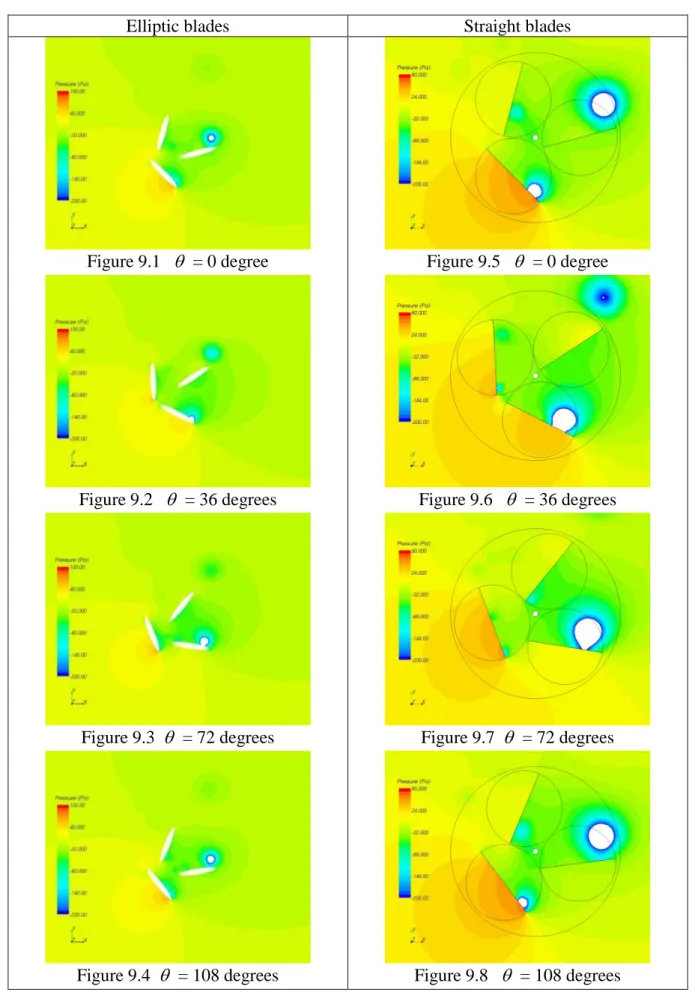
Elliptic blades Straight blades

Figure 9.1  = 0 degree Figure 9.5  = 0 degree

Figure 9.2  = 36 degrees Figure 9.6  = 36 degrees

Figure 9.3  = 72 degrees Figure 9.7  = 72 degrees

Figure 9.4  = 108 degrees Figure 9.8  = 108 degrees

Elliptic blades Straight blades

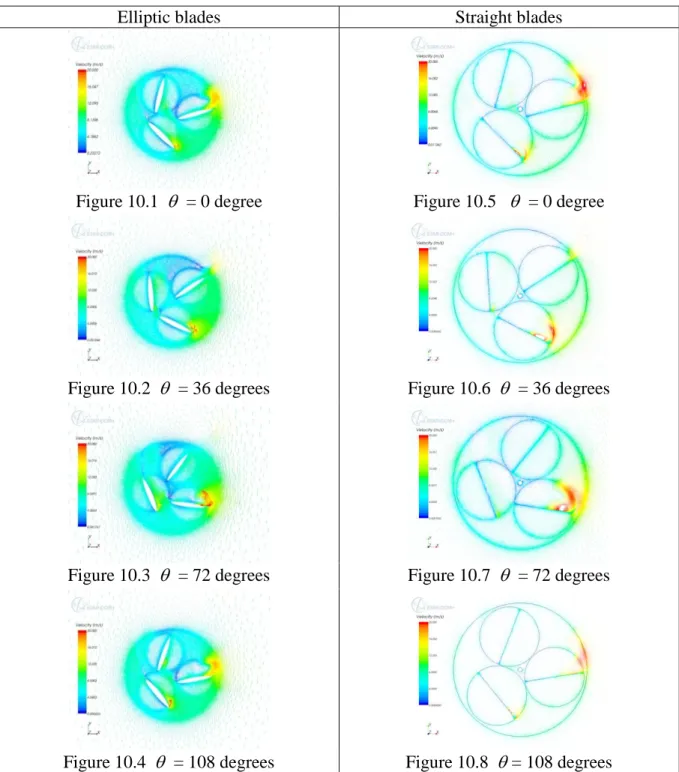
Figure 10.1  = 0 degree Figure 10.5  = 0 degree

Figure 10.2  = 36 degrees Figure 10.6  = 36 degrees

Figure 10.3  = 72 degrees Figure 10.7  = 72 degrees

Figure 10.4  = 108 degrees Figure 10.8  = 108 degrees

Figures 10: Vectors fields = 15;  = 0.6; Re = 560 000

Figures 7 give contours of relative pressure for an initial blade stagger angle of 0 degrees for the two kinds of blades for  = 0.4. Figures 8 give same results for  = 0 and  = 0.6 and figures 9 for  = 15 and  = 0.6. For these different values, results are periodic with no highly instabilities. So, only results between 0 to 120 degrees are presented, corresponding to one periodicity.

Scale, between – 200 to 100 Pa, is used for elliptic blades and scale between -200 to 80 Pa, for straight blades.

Comparison between two kinds of profiles shows quite same behaviours but emphasized in case of straight blades.

For each kind of blades, a swirl arises at the leading edge of the lower blade. This swirl grows up when the blade rotates and breaks off blade for azimuth angle of blade  equal about -14 degrees. Then it reduces until vanished for  equal about 90 degrees. In figure 9.3, two swirls can be observed, the first, near the leading edge, which has broken off the blade and the second, quite above the first, which is vanishing. This can be observed more accurately for an initial blade stagger angle of 15 degrees (Figures 9)

Figure 10.1 to 10.4 give vectors field for elliptic blades and Figure 10.5 to 10.8 give same results for straight blades for a speed ratio of 0.6, for a blade stagger angle of 15 degrees. Same scale is used for vectors fields: between 0 to 20 m/s. For all cases, flow is repeating so period is divided by three as it can be observed. But, in order to compare results, same azimuth angle were chosen to be presented. Comparisons between Figures 10.1-10.4 to Figures 10.5-10.8 point up that each blade has not a great influence on the other blades: stream around each blade seems to be no influenced by the stream around the other blades. Same behaviour between elliptic and straight blades can be observed. Maximum velocity occurs for azimuth angle between -120 degrees to 30 degrees. Maximum velocity is greater for straight blades.

As it can be observed in the previous studies, blades for azimuth angle between 90 to 250 degrees seem to slide in the flow field avoiding to disturb the flow stream of the wind and avoiding to generate a great negative torque as it can be seen in figures 6.

The examination of vectors fields shows the interest of a blade stagger angle near 0 degrees, because, for other angles, the effect of sliding of blades decreases and range of negative torques increases.

These remarks are also true when blade speed ratios are not in agreement with blade stagger angles.

These analysis leads to some new ways of investigation: - Analytical study of influence parameters if possible - Spectral analysis of recording results

CONCLUSION

New numerical experiments were carried out to study the influence of different blades on the performance of turbine with rotating blades. The following conclusions have been drawn: - The performance of this kind of turbine was confirmed to be very good and better than those of classical VAWTs for some specific blade stagger. The maximum mean numerical coefficient at a blade speed ratio equal to 0.4 was about 38%.

- Each blade’s behaviour seems to have less influence on flow stream around next blade and on power performance.

- A significant influence of sketch of blades depending on other parameters like blade speed ratios and initial blade stagger angles.

- A significant influence of blade speed ratios

- A significant influence of initial blade stagger angle

A wide range of results have been obtained and still needs more analyses to understand all what happens in this VAWT. A lot of work has still to be done: influence of number and relative position (radius of centre) of blades, analytical analysis, spectral analysis…

NOMENCLATURE

Cp Power coefficient (no units)

Ceff Real torque (mN)

D Diameter of turbine zone (m)

Rt Radius of blade tip, m

S Captured swept area, m2 V0 Wind velocity, =8 m/s

Gi Centre of rotation of blade i

L Length of blade (m)

Mti Torque of blade i by turbine axis, mN

O Centre of rotation of turbine in 2D model Peff Real power

R Radius of axis of blades, =0.62 m Re Reynolds number based on length of

blade

 Blade stagger angle (degrees)

 Blade or tip blade speed ratio (no units)

 Density of air, kg/m3

 Azimuth angle of blade 1(degrees)

1 Angular velocity of turbine (rad/s)

2 Angular velocity of pales (rad/s)

Subscripts i Blade index LITERATURE

Leconte P., Rapin M., Szechenyi E., Eoliennes, Techniques de l’ingénieur BM 4 640,, pp 1-24, 2001

Martin J., Energies éoliennes, Techniques de l’ingénieur B 8 585, pp 1-21, 1987 Hau E., Wind turbines, Springer, Germany, 2000

Paraschivoiu I., Wind Turbine Design with Emphasis on Darrieus Concept , Polytechnic International Press, 2002

Pawsey N.C.K., Development and evaluation of passive variable-pitch vertical axis wind turbines, PhD Thesis, Univ. New South Wales, Australia, 2002

P.A.M. Dieudonné P.A.M., Eolienne à voilure tournante à fort potentiel énergétique , Demande de brevet d’invention FR 2 899 286 A1, brevet INPI 0602890, 2006

Cooper P., Kennedy 0., Development and analysis of a novel Vertical Axis Wind Turbine,

http://www.datataker.com/public_domain/PD71%20Development%20and%20analysis%20of

%20a%20novel%20vertical%20axis%20wind%20turbine.pdf, Accessed on September 2010

Cooper P., Wind Power Generation and wind Turbine Design , WIT Press, chapitre 8, ISBN 978-1-84564-205-1, 2010

Bayeul-Lainé A. C., Bois G., Simonet S., Etude numérique instationnaire d’une micro-éolienne à axe vertical , 1ère Conférence Franco syrienne sur les énergies renouvelables, octobre , Damas, Syrie, 2010

Bayeul-Lainé A.C., Bois G., Unsteady simulation of flow in micro vertical axis wind turbine , Proceedings of 21st International Symposium on Transport Phenomena, Kaohsiung City Taiwan, 02-05 November 2010

Marchaj C. A., The Aero-Hydrodynamics of Sailing, International Marine Publishing Company, ISBN 0229986528, 2000