The first-digit frequencies in data of turbulent flows

Science Arts & Métiers (SAM)

is an open access repository that collects the work of Arts et Métiers Institute of

Technology researchers and makes it freely available over the web where possible.

This is an author-deposited version published in:

https://sam.ensam.eu

Handle ID: .

http://hdl.handle.net/10985/9977

To cite this version :

Damien BIAU - The first-digit frequencies in data of turbulent flows - Physica A - Vol. 440,

p.147–154 - 2015

Any correspondence concerning this service should be sent to the repository

Administrator :

archiveouverte@ensam.eu

The first-digit frequencies in data of turbulent flows

Damien Biau

DynFluid Laboratory, Arts et Métiers ParisTech, 151 Boulevard de l’Hôpital, 75013 Paris, France

Keywords:

Turbulent flow First significant digit Shannon’s entropy Dissipation Spectral method

a b s t r a c t

Considering the first significant digits (noted d) in data sets of dissipation for turbulent flows, the probability to find a given number (d=1 or 2 or . . . 9) would be 1/9 for a uni-form distribution. Instead the probability closely follows Newcomb–Benford’s law, namely

P(d) =log(1+1/d). The discrepancies between Newcomb–Benford’s law and first-digits frequencies in turbulent data are analysed through Shannon’s entropy. The data sets are obtained with direct numerical simulations for two types of fluid flow: an isotropic case initialized with a Taylor–Green vortex and a channel flow. Results are in agreement with Newcomb–Benford’s law in nearly homogeneous cases and the discrepancies are related to intermittent events. Thus the scale invariance for the first significant digits, which supports Newcomb–Benford’s law, seems to be related to an equilibrium turbulent state, namely with a significant inertial range. A matlab/octave program provided in appendix is such that part of the presented results can easily be replicated.

1. Introduction

In 1881 Newcomb [1] observed a rather strange fact: tables of logarithms in libraries tend to be quite dirty at the beginning and progressively cleaner throughout. This seemed to indicate that people had more occasions to calculate with numbers beginning with 1 than with other digits. Newcomb concluded that the frequency of the leftmost, nonzero digit d closely follows the probability law:

P

(

d

) =

log₁₀



1

+

1 d



d

=

1

,

2

, . . .

9

.

(1)

Hence the numbers in typical statistics should have a first digit of 1 about 30% of the time, but a first digit of 9 only about 4.6% of the time (the other values can be found inTable 1). Also, the probability that the first significant digit is an odd number is 60%. This formula is also valid for the digits beyond the first, for example the distribution of the k first digits is given by Eq.(1)with d

=

10k−1

, . . .

10k

−

1.

Newcomb’s article went unnoticed until 1938 when Benford [2] has independently followed the same path: starting from observations about logarithm books, he deduced the same law. Benford also noted that this law is base-invariant, the definition(1)is given here with a decimal representation (base-10) for convenience. Until today this empirical law has been tested against various data sets ranging from mathematical curiosity to natural sciences [3,4].

Then there have been many attempts to rationalize this empirical law [5–10]. Recently Fewster [10] has provided an intuitive explanation based on the fact that any distribution has tendency to satisfy Newcomb–Benford’s law, as long as the distribution spans several orders of magnitude and as long as the distribution is reasonably smooth.

Pietronero et al. [7] have shown that Newcomb–Benford’s law is equivalent to the scale invariance of data set. Multiplying a data set X by a factor

λ

rescales the first-digits distribution such that: P

(

d

[

λ

X

]

) = λ

m_P

₍

_d

_[

_X

_]

₎

_{, where d}

_[

_X

_]

_{denotes the first}

significant digit of the variable X and m is an exponent to be determined. The general solution of this equation takes the form of power-law. The probability distribution P

(

d

)

, namely the sub-interval of

[

1

,

10

)

occupied by the first digit d, is obtained by integration:

P

(

d

) =

K



d+1

d

z−αdz

where K is a necessary constant to enforce the condition



P

=

1. Newcomb–Benford’s law is recovered for

α =

1, while

α ̸=

1 leads to the generalized distribution found by Pietronero et al. [7]:

P

(

d

) =

(

d

+

1

)

1−α

₋

_d1−α

101−α

₋

₁

.

(2)

The generalized Newcomb–Benford law has been applied to the distribution of leading digits in the prime number sequence by Luque and Lacasa [11], the results have shown an asymptotic evolution towards the uniform distribution (

α =

0). Note that as particular case

α =

1, Newcomb–Benford’s law satisfies a strong invariance, i.e. P

(

d

[

λ

X

]

) =

P

(

d

[

X

]

)

. This result was first demonstrated by Hill [6]. As illustration, we consider X such that d

[

X

] =

7 and

λ =

2 as scaling factor, thus d

[

λ

X

] =

1, but the secondary digit can only be 4 or 5. With the relation(1), it is easy to check the scale-invariance for this example:

P

(

7

) =

P

(

14

) +

P

(

15

)

.

Self-similarity is also a well explored topic in turbulent flows. The first step was made by Richardson in the late 19th century with the assumption of a universal cascade process of the energy: the energy input at large scale is successively transferred to finer eddies. This idea has been refined by Kolmogorov and Obukhov, the cascade is then assumed to occur in a space-filling, self-similar way. Formally there should be a unique scaling exponent for the structure functions S

(

r

)

such that S

(λ

r

) = λ

h_S

₍

_r

₎

_{. Today the departures from the Kolmogorov scaling prediction are identified to different causes: the}

Reynolds number is not large enough, the flow is not exactly isotropic or the self-similarity assumption is not valid. The last point is related to the intermittent feature of the cascade process, resulting in anomalous scaling, or no unique scaling exponent. Further information can be found in the book by Frisch [12].

In the present work, the distribution of first significant digits is used as an alternative statistical tool for analysing turbulent flows. Newcomb–Benford’s law is compared to data sets coming from numerical simulations of the Taylor–Green vortices (homogeneous case) and the plane Poiseuille flow (inhomogeneous case). In the next section the numerical method is presented and the Shannon entropy is introduced as a diagnostic tool. Results are presented in the following section. The validity and the possible extensions of the method are discussed in the last section.

2. Method

The momentum and mass conservation equations applied to the fluid lead to the Navier–Stokes equations, written in non dimensional form:

∇ ·

u

=

0

,

∂

tu

+

u

· ∇

u

= −∇

p

+

Re−1

∇

2u

(3) the flow is assumed incompressible and the Reynolds number (Re) is the only control parameter.

It should be noted that the quadratic nonlinear term in the Navier–Stokes equations can be related to Newcomb– Benford’s law. If we assume a scale invariant data set, then the peculiar Newcomb–Benford’s law could be rooted in this non-linear term. Let consider the quadratic transformation, X

→

X2, mimicking the nonlinear convective term in Navier–Stokes equations(6). The probability to find the first digit of X in the interval

[

d

,

d

+

1

)

equals the probability to find the first digit of X2_in

_[

_d2

_{, (}

_d

₊

₁

₎

2

₎

_:



(d+1)2 d2 z− ˜αdz

=



d+1 d z−αdz

leading to

α = (α +

˜

1

)/

2. For any distribution, characterized by an exponent

α

, the quadratic transformation generates a distribution with an exponent

α

˜

which is closer to 1 than initial

α

. As a consequence the quadratic non-linear term

Fig. 1. Entropy for various distributions. Newcomb–Benford’s case, marked with a solid circle, corresponds toα =1 and H=0.8657.

in Navier–Stokes equations(6) acts as a feedback which forces any scale invariant distribution (any

α

) towards New-comb–Benford’s law (

α =

1). However the underlying reason why scale invariance occurs is still elusive. As stated by Fewster [10], currently any argument can explain why a universal law of nature should arise in the first place.

Now we have to choose the observable which will be used to apply the statistical analysis. The viscous dissipation has been selected:

ϵ =

1 Re 1 2



∂

ui

∂

xk

+

∂

uk

∂

xi



2

.

(4)

In a practical point of view, the dissipation in internal or external flow fields is directly related to friction factor and drag coefficient respectively. In addition, for isothermal flows, the dissipation is the only term responsible for entropy production. Hence the dissipation can be considered as cornerstone for turbulent statistics, for a recent overview see Vassilicos [13]. The dissipation appears as a natural choice in order to exemplify the first-digit statistics in turbulent flows.

In order to investigate the possible conformance of turbulent data to Newcomb–Benford’s law, it is necessary to quantify their discrepancy. This can be achieved through different ways. First by using the usual statistical tools to test the goodness of fit, for example the

χ

2_{or chi-square test. Secondly the search of the optimal exponent}

_α

_{in the generalized distribution,}

Eq.(2), see Luque and Lacasa [11]. Eventually a third choice was retained, stemming from the information theory. In 1948 Shannon [14] introduced entropy as a measure of the uncertainty in a random variable:

H

= −

9



d=1

P

(

d

)

log₁₀P

(

d

).

(5)

This definition of entropy is associated to lack of information or to uncertainties. A message, in our case a chain of first digits d, occurring with probability P

(

d

)

, contains the information I

= −

log₁₀P

(

d

)

. Thus Shannon entropy H may be seen as the information averaged over the message space. That formula can be heuristically explained considering the fact that total information of two independent events (with respective probabilities P1and P2) is the sum of the two individual information,

namely I

(

P1

,

P2

) =

I

(

P1

) +

I

(

P2

)

, hence the logarithm. Moreover information is a positive quantity, hence minus sign, and

the information contained in certain events vanishes: I

(

1

) =

0.

The Shannon entropy applied to the general probability distribution (Eq.(2)) is depicted inFig. 1.

The maximum entropy is achieved when all digits are equally probable. The principle of maximum entropy leads to the notion of equipartition: the equal spread of probabilities over all possible states of a system. InFig. 1, the maximum value is H

=

log₁₀

(

9

) ≈

0

.

9542. Conversely the minimum entropy occurs when one digit is certain, then entropy vanishes.

The extensive property of entropy is straightforward if we consider Newcomb–Benford’s law for digits beyond the first. Hill [3] has shown that the probability P that d

(

d

=

0

,

1

, . . . ,

9

)

is encountered as the nth (n

>

0) digit is:

Pn

(

d

) =

10n₋₁



k=10n−1 log₁₀



1

+

1 10k

+

d



.

The distributions of the first and second digits are not independent, however, as n increases, the distributions of successive digits become independent and rapidly converge to an even distribution (p

=

0

.

1 for each of the ten digits). Thus, for sufficiently large n, the entropy satisfies the extensive property:

H

(

Pn

,

Pn+1

) =

H

(

Pn

) +

H

(

Pn+1

) →

2 as n

→ ∞

.

3. Results

In the following, two turbulent flows are considered. First a three-dimensional decaying and homogeneous turbulent flow, initialized with a Taylor–Green vortex. Then a developed wall-bounded turbulent flow in a plane channel.

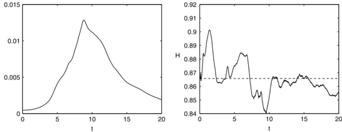
Fig. 2. Left: Rate of energy dissipationϵas a function of time for Re=1600. Right: Shannon entropy vs. t for the Taylor–Green vortex. The dotted line stands for the Shannon entropy corresponding to Newcomb–Benford’s law, H=0.8657.

Fig. 3. Comparisons between Newcomb–Benford’s law (filled bar) and the probability distribution of the first significant digits of dissipation for the

Taylor–Green vortex (empty bar), at t=10 (left) and t=20 (right). 3.1. Homogeneous and isotropic case: the Taylor–Green vortex

We consider a spatially periodic flow, the problem is studied by direct numerical simulation with 2563_{Fourier modes}

and the Reynolds number is Re

=

1600. As initial condition we impose the single-mode Taylor–Green vortex [15,16]:

u

(

x

,

y

,

z

,

t

=

0

) =

2

/

√

3 sin

(

2

π/

3

)

sin x cos y cos z

v(

x

,

y

,

z

,

t

=

0

) = −

2

/

√

3 sin

(

2

π/

3

)

cos x sin y cos z

w(

x

,

y

,

z

,

t

=

0

) =

0

.

(6)

This initial solution generates a very complex flow and evolves into turbulent flow for sufficiently high Reynolds number. The small scales are generated by three-dimensional vortex stretching, as described in the original article by Taylor and Green [15]. Because of deterministic nature of the Navier–Stokes equations, the flow issuing from a Taylor–Green vortex presents microscopic structure which can be reproduced repeatedly. The results presented hereafter can thus be easily reproduced with the program provided in Appendix.

The time evolution of the total dissipation and the conformance of turbulent statistics with Benford’s law are presented inFig. 2.

The transient increase of the dissipation, until its maximum value reached at t

≈

9, characterizes the nonlinear vortex stretching followed by an overall decay of the flow by viscous effect. For further details see Brachet et al. [16]. Shannon’s entropy slightly oscillates around the value expected from Newcomb–Benford’s law, namely H

=

0

.

8657. The first-digit frequencies are close to Newcomb–Benford’s distribution, which is confirmed by a direct comparison shown inFig. 3.

3.2. Non-homogeneous case: the plane Poiseuille flow

Next consider a turbulent plane Poiseuille flow, namely a channel flow driven by a streamwise pressure gradient, at two different Reynolds numbers: Re

=

2800 and Re

=

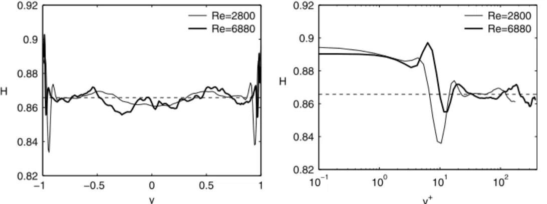
6880. The Reynolds number is defined with the half-height of the channel and the bulk velocity. The no-slip boundary condition on the walls induces a different scaling based on the friction velocity

Fig. 4. Shannon entropy as a function of wall distance y (left) and wall distance in wall units y+_{(right). Results for the turbulent plane Poiseuille flow,}

for two Reynolds number values: Re = 2800 (thin line) and Re = 6880 (thick line). The dashed line represents the entropy value corresponding to Newcomb–Benford’s law, namely H=0.8657.

Table 1

Probability distribution P(d)for the first significant digits. Distribution given by Newcomb–Benford’s law (N–B) and distributions extracted from dissipation data for the turbulent plane Poiseuille flow.

Digit Newcomb–Benford’s law Plane Poiseuille flow Plane Poiseuille flow

Re=2800 Re=6880 1 0.3010 0.2892 0.2995 2 0.1761 0.1777 0.1724 3 0.1249 0.1297 0.1238 4 0.0969 0.1011 0.0973 5 0.0792 0.0820 0.0804 6 0.0669 0.0682 0.0684 7 0.0580 0.0579 0.0594 8 0.0512 0.0501 0.0523 9 0.0458 0.0442 0.0466

number values based on the skin friction velocities become Re_τ

=

180 and Re_τ

=

395, respectively. The scale separation between the inner layer and the outer layer increases with Reynolds number, thus it appears useful to analyse the channel flow for two Reynolds number values. The numerical parameters are those used in Kim et al. [17] and Moser et al. [18].

Results are temporally averaged and the conformance of turbulent statistics with Benford’s law is represented, respectively to the wall distance expressed in outer scaling y and in wall units y+, in Fig. 4.

Again, first-digit frequencies slightly oscillate around Newcomb–Benford’s distribution, except in the near-wall region where the oscillation amplitudes are stronger. In fact, Toschi et al. [19] have observed maximum intermittency effects in that near-wall region, where it is known that the bursting phenomenon is the dominant dynamical feature. In addition, Toschi et al. [19] found that for positions close to the channel centreline, scaling exponents are in substantial agreement with observations in homogeneous and isotropic turbulence.

Shannon’s entropy has been used as diagnostic tool to quantify the discrepancy with Newcomb–Benford’s law. Moreover, this information entropy can also be seen as a numerical measure which describes how informative a particular probability distribution is, ranging from zero (completely uninformative) to Hmax

=

log10 9

≈

0

.

9542 (completely informative). With

this point of view, the conclusion above is consistent with results presented by Cerbus and Goldburg [20,21]. Cerbus and Goldburg observed, from experiments in a turbulent soap film, that turbulence is easier to predict where a cascade exists, or equivalently, for flows with a significant inertial range. They also found that the spatial information-entropy density is a decreasing function of the Reynolds number.

In order to complete the previous qualitative comparisons, a quantitative comparison is presented in Table 1.

Various tests on the numerical parameters have been realized in order to check the robustness of the presented results. Results remain qualitatively unchanged after: varying the spatial or temporal discretization, or interpolating data on different meshes, or increasing the domain size. Thus presented results seem to be free from possible numerical biases.

4. Discussion

In conclusion first-digit statistics closely follow Newcomb–Benford’s law. This is especially true when an equilibrium is reached: during the decay of homogeneous turbulent flows or in the far from walls region of channel flows. The scale-invariant property constituting Newcomb–Benford’s law seems to be satisfied in conjunction with the eddies cascade in the inertial range.

The law of first digits is not just a mathematical curiosity, the most practical use for Newcomb–Benford’s law is in fraud detection [22], or the possible detection of earthquakes [4]. In the framework of turbulent flows, a practical application of

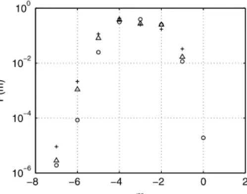
Fig. 5. Probability mass function for the exponent m in dissipation data for the Taylor–Green vortex at t=10 (◦), Plane Poiseuille at Re=2800(△)and

Re=6880(+).

first-digits statistics could be in the reduced-order models assessment, which could be investigated through their ability to conserve the first-digit frequencies (see Tolle et al. [23]).

Finally the approach described in the present article can be generalized by considering the general form of scientific notation:

±

X 10m

.

(7)

The first significant digit d

(

X

)

is the object of the present study and the two other parameters (namely the sign and the exponent) can also be analysed statistically. For the dissipation, the sign is always positive (see Eq.(4)), nonetheless for other quantities, for example the velocity fluctuations, the sign-change statistics provide interesting information. Indeed the time scale related to the fluctuating velocity zero-crossing is approximately equal to the Taylor scale in turbulent flows (see Kailasnath et al. [24] and references within). The last parameter in the formula(7)is the power m. The distributions of the power m, for the different flows considered here, are shown in Fig. 5.

Despite variety of the flow configurations, the curves look very similar. However in lack of theoretical background (as far as I know), it is not possible to go deeper into the analysis, letting that as an open issue.

Acknowledgement

The author wishes to thank Eric Lamballais for the stimulating discussions on the subject and for his insightful remarks about the present manuscript.

Appendix A. MatLab–Octave program to compute the first-digit frequencies

function P=NewcombBenford(X); X=abs(X);

fd = floor(X./(10.

ˆ

floor(log10(X)))); % extract the first digit P = histc(fd,1:9)’/length(X); % probability

Appendix B. MatLab–Octave program for the Taylor–Green vortex simulation

We here consider the flow of an incompressible fluid under periodic boundary conditions with period 2

π

. The pressure term can be eliminated by the incompressibility condition, then Navier–Stokes equations can be written as:

∂

u

∂

t

=

u

×

ω − ∇



p

+

1 2u 2



+

Re−1

∇

2u

where

ω = ∇ ×

u is the vorticity. Time marching is realized with Fourth-order Runge–Kutta method and alias error is

removed by mode truncation (Orszag 2/3 rule). %%——————————————————————-%% simulation of Taylor–Green Vortex %%——————————————————————-clear all,

Re = 1600; N = 2

ˆ

8; dt = 5e-3;

Tend=20;

%——————————————————————-%% Fourier pseudo-spectral method

x = 2*pi/N*[0:N-1]’; kx = [0:N/2-1 0 -N/2+1:-1]’; for m=1:N, for n=1:N,

IKX(:,m,n)=i*kx; IKY(m,:,n)=i*kx; IKZ(m,n,:)=i*kx; end, end

K2=-(IKX.

ˆ

2+IKY.

ˆ

2+IKZ.

ˆ

2);

K2p=K2; K2p(1,1,1)=1; K2p(N/2+1,:,:)=1; K2p(:,N/2+1,:)=1; K2p(:,:,N/2+1)=1; Z=ones(N,N,N); Z(N/2+1,:,:)=0; Z = 1 - (sqrt(K2)

>

round(N/3)+1); Z(:,N/2+1,:)=0; Z(:,:,N/2+1)=0; E = exp(-dt*K2/Re); E2 = exp(-dt/2*K2/Re); %% Newcomb–Benford’s law NBL=log10(1+1./[1:9]); SNB(1)=-sum(NBL.*log10(NBL)); %% initial condition [Xs

,

Ys

,

Zs] = meshgrid(x,x,x); %% 3D grid uf = fftn( 2/sqrt(3)*sin( 2*pi/3)*sin(Xs).*cos(Ys).*cos(Zs) ); vf = fftn( 2/sqrt(3)*sin(-2*pi/3)*cos(Xs).*sin(Ys).*cos(Zs) ); wf = zeros(N,N,N); clear Xs Ys Zs for k=1:round(Tend/dt) %%=========================== u=real(ifftn(uf)); v=real(ifftn(vf)); w=real(ifftn(wf));

nltu=Z.*fftn(v.*real(ifftn(IKX.*vf-IKY.*uf))-w.*real(ifftn(IKZ.*uf-IKX.*wf))); nltv=Z.*fftn(w.*real(ifftn(IKY.*wf-IKZ.*vf))-u.*real(ifftn(IKX.*vf-IKY.*uf))); nltw=Z.*fftn(u.*real(ifftn(IKZ.*uf-IKX.*wf))-v.*real(ifftn(IKY.*wf-IKZ.*vf))); pf=-(IKX.*nltu+IKY.*nltv+IKZ.*nltw)./K2p; pf(1,1,1)=0;

nltu=nltu-IKX.*pf; ufa = E2.*(uf + dt/2*nltu); nltv=nltv-IKY.*pf; vfa = E2.*(vf + dt/2*nltv); nltw=nltw-IKZ.*pf; wfa = E2.*(wf + dt/2*nltw); u=real(ifftn(ufa)); v=real(ifftn(vfa)); w=real(ifftn(wfa));

nltua=Z.*fftn(v.*real(ifftn(IKX.*vfa-IKY.*ufa))-w.*real(ifftn(IKZ.*ufa-IKX.*wfa))); nltva=Z.*fftn(w.*real(ifftn(IKY.*wfa-IKZ.*vfa))-u.*real(ifftn(IKX.*vfa-IKY.*ufa))); nltwa=Z.*fftn(u.*real(ifftn(IKZ.*ufa-IKX.*wfa))-v.*real(ifftn(IKY.*wfa-IKZ.*vfa))); pf=-(IKX.*nltua+IKY.*nltva+IKZ.*nltwa)./K2p; pf(1,1,1)=0;

nltua=nltua-IKX.*pf; ufb = E2.*(uf + dt/2*nltua); nltva=nltva-IKY.*pf; vfb = E2.*(vf + dt/2*nltva); nltwa=nltwa-IKZ.*pf; wfb = E2.*(wf + dt/2*nltwa); u=real(ifftn(ufb)); v=real(ifftn(vfb)); w=real(ifftn(wfb));

nltub=Z.*fftn(v.*real(ifftn(IKX.*vfb-IKY.*ufb))-w.*real(ifftn(IKZ.*ufb-IKX.*wfb))); nltvb=Z.*fftn(w.*real(ifftn(IKY.*wfb-IKZ.*vfb))-u.*real(ifftn(IKX.*vfb-IKY.*ufb))); nltwb=Z.*fftn(u.*real(ifftn(IKZ.*ufb-IKX.*wfb))-v.*real(ifftn(IKY.*wfb-IKZ.*vfb))); pf=-(IKX.*nltub+IKY.*nltvb+IKZ.*nltwb)./K2p; pf(1,1,1)=0;

nltub=nltub-IKX.*pf; ufb = E.*(ufa + dt*nltub); nltvb=nltvb-IKY.*pf; vfb = E.*(vfa + dt*nltvb); nltwb=nltwb-IKZ.*pf; wfb = E.*(wfa + dt*nltwb); u=real(ifftn(ufb)); v=real(ifftn(vfb)); w=real(ifftn(wfb));

nltuc=Z.*fftn(v.*real(ifftn(IKX.*vfb-IKY.*ufb))-w.*real(ifftn(IKZ.*ufb-IKX.*wfb))); nltvc=Z.*fftn(w.*real(ifftn(IKY.*wfb-IKZ.*vfb))-u.*real(ifftn(IKX.*vfb-IKY.*ufb))); nltwc=Z.*fftn(u.*real(ifftn(IKZ.*ufb-IKX.*wfb))-v.*real(ifftn(IKY.*wfb-IKZ.*vfb))); pf=-(IKX.*nltuc+IKY.*nltvc+IKZ.*nltwc)./K2p; pf(1,1,1)=0;

nltvc=nltvc-IKY.*pf; nltwc=nltwc-IKZ.*pf;

uf = E.*(uf + dt/6*(nltu + 2*(nltua+nltub) + nltuc)); vf = E.*(vf + dt/6*(nltv + 2*(nltva+nltvb) + nltvc)); wf = E.*(wf + dt/6*(nltw + 2*(nltwa+nltwb) + nltwc));

%% plot result time(k) = k*dt;

EPS=(2*(real(ifftn(IKX.*uf)).

ˆ

2+real(ifftn(IKY.*vf)).

ˆ

2+ ... real(ifftn(IKZ.*wf)).

ˆ

2)+real(ifftn(IKY.*uf + IKX.*vf)).

ˆ

2+ ...

real(ifftn(IKZ.*vf + IKY.*wf)).

ˆ

2+real(ifftn(IKX.*wf + IKZ.*uf)).

ˆ

2)/Re; Diss(k) = mean(mean(mean(EPS)));

X = reshape(EPS,N

ˆ

3,1);

fd = floor(X./(10.

ˆ

floor(log10(X)))); % extract the first digit stat(:,k) = histc(fd,1:9)’/length(X); % compute the probability H(k)=-sum(stat(:,k).*log10(stat(:,k)));

div = max(max(max(abs( real(ifftn(IKX.*uf+IKY.*vf+IKZ.*wf)) ))));

disp([’ time=’,num2str(time(k)),’ divergence=’,num2str(div),’ dissipation=’,num2str(Diss(k))]) subplot(1,2,1), plot(time,Diss), xlabel t, ylabel dissipation

subplot(1,2,2), plot(time,H,[0 time(k)],SNB*[1 1],’k’), xlabel t, ylabel H drawnow,

end % TIME STEPPING =================================

References

[1]S. Newcomb, Note on the frequency of use of the different digits in natural numbers, Amer. J. Math. 4 (1881) 39–40.

[2]F. Benford, The law of anomalous numbers, Proc. Am. Phil. Soc. 78 (1938) 551–572.

[3]T.P. Hill, The first digit phenomenon, Am. Sci. 86 (1998) 358–363.

[4]M. Sambridge, H. Tkalcic, A. Jackson, Benfords law in the natural sciences, Geophys. Res. Lett. 37 (2010) L22301.

[5]R.A. Raimi, The first digit problem, Amer. Math. Monthly 83 (1976) 521–538.

[6]T.P. Hill, A statistical derivation of the significant-digit law, Statist. Sci. 10 (1995) 354–363.

[7]L. Pietronero, E. Tosatti, V. Tosatti, Vespignani, Explaining the uneven distribution of numbers in nature: the laws of Benford and Zipf, Physica A 293 (2001) 297–304.

[8]R.S. Pinkham, On the distribution of first significant digits, Ann. Math. Statist. 32 (1961) 1223–1230.

[9]A. Pocheau, The significant digit law: a paradigm of statistical scale symmetries, Eur. Phys. J. B 49 (2006) 491–511.

[10]R.M. Fewster, A simple explanation of Benford’s Law, Amer. Statist. 63 (2009) 26–32.

[11]B. Luque, L. Lacasa, The first-digit frequencies of prime numbers and Riemann zeta zeros, Proc. R. Soc. A 465 (2009) 2197–2216.

[12]U. Frisch, Turbulence. The Legacy of A. N. Kolmogorov, Cambridge University Press, 1995.

[13]J.C. Vassilicos, Dissipation in turbulent flows, Annu. Rev. Fluid Mech. 47 (2015) 95–114.

[14]C.E. Shannon, A mathematical theory of communication, Bell Syst. Tech. J. 27 (1948) 379–423.

[15]G.I. Taylor, A.E. Green, Mechanism of the production of small eddies from large ones, Proc. R. Soc. A Math. Phys. Sci. 158 (1936) 499–521.

[16]M.E. Brachet, D.I. Meiron, S.A. Orszag, B.G. Nickel, R.H. Morf, U. Frisch, Small-scale structure of the Taylor–Green vortex, J. Fluid Mech. 130 (1983) 411–452.

[17]J. Kim, P. Moin, R. Moser, Turbulence statistics in fully developed channel flow at low Reynolds number, J. Fluid Mech. 177 (1987) 133–166.

[18]R.D. Moser, J. Kim, N.N. Mansour, Direct numerical simulation of turbulent channel flow up to Re=590, Phys. Fluids 11 (1999) 943–945.

[19]F. Toschi, G. Amati, S. Succi, R. Benzi, R. Piva, Intermittency and structure functions in channel flow turbulence, Phys. Rev. Lett. 82 (1999) 5044.

[20]R.T. Cerbus, W.I. Goldburg, Information content of turbulence, Phys. Rev. E 88 (2013) 053012.

[21]R.T. Cerbus, W.I. Goldburg, Predicting two-dimensional turbulence, Phys. Rev. E 91 (2015) 043003.

[22]M. Nigrini, A taxpayer compliance application of Benford’s law, J. Am. Tax Assoc. 18 (1996) 72–91.

[23]C.R. Tolle, J.L. Budzien, R.A. LaViolette, Do dynamical systems follow Benford’s law? Chaos 10 (2000) 331–336.